Study of color superconductivity with Ginzburg-Landau effective action on the lattice

Abstract

We study thermal phase transitions of color superconductivity by the lattice simulations of the Ginzburg-Landau (GL) effective theory. The theory is equivalent to the SU_f(3) $\times$ SU_c(3) Higgs model coupled to SU_c(3) color gauge fields. From the eigenvalues of a 3$\times$3 gauge-invariant diquark composite, a clear distinction between the 2-flavor color superconductivity (2SC) and the color flavor locking (CFL) phase is made in a gauge invariant manner. The thermal transitions between the normal phase and the superconducting phases are found to be first-order due to thermal gluons. The phase structure in the coupling-constant space is numerically explored and three patterns of phase transition, i.e., normal$\rightarrow$2SC, normal$\rightarrow$CFL and normal$\rightarrow$2SC$\rightarrow$CFL, are found in the chiral limit. These results agree qualitatively with the weak-coupling analysis of the GL theory.

TKYNT-05-29, IMSc/2005/11/26

1 Introduction

In dense and cold quark matter, color superconducting phase is expected to be realized due to diquark pairing (see the reviews, [1]). From the analysis of the pairing interaction, the most attractive channel is found to be in the color anti-triplet and $J^{P}=0^{+}$ channel, which leads to the diquark field, $\varPhi_{cf}=\epsilon_{abc}\epsilon_{fjk}\langle q^{j}\!\!_{a}{\rm C}\gamma_{5}q^{k}\!\!_{b}\rangle$, as the most relevant quantity to describe color superconductivity. A three-dimensional Ginzburg-Landau (GL) effective action written in terms of $\varPhi_{cf}$ was proposed [2] to study the thermal phase transition of the color superconductivity. Then, it was realized that the thermal gluons (treated in weak-coupling approximation) turn the second-order transition in the mean-field theory to the first order transition [3, 4]. Such a weak-coupling study, however, is valid only in extremely high density because the gauge coupling grows for small baryon density. Furthermore, thermal fluctuations of the diquark field become also important as density decreases [3].

Motivated by this observation, we carry out Monte-Carlo simulations of the GL effective action discretized on the lattice. Although the simulation of the GL effective action is not ab initio calculation and is applicable only near the thermal phase boundary, it has an advantage of making non-perturbative calculation and simultaneously of avoiding the sign problem which is a serious obstacle in direct lattice QCD simulation at finite density. Since the GL action has color SU_c(3) gauge invariance and the diquark field $\varPhi_{cf}$ is a gauge variant object, it is not a trivial task to identify the color superconducting phase in the lattice approach. We will see below that the eigenvalues of a gauge invariant composite $\sum_{x}\varPhi^{\dagger}_{x}\varPhi_{x}$ are useful to identify different phases. ($x$ denotes lattice sites.) Also, analyzing the hysteresis loops of such gauge invariant observables, we find the first-order transitions among these phases.

2 The Ginzburg-Landau effective action

The 3-dimensional Ginzburg-Landau (GL) action in the chiral limit [2], which is expected to be universal around the thermal phase boundary, reads $S_{\rm GL}=\int d^{3}x{\cal L}$ with

$${\cal L}=\frac{m^{2}}{2}{\rm Tr}(\varPhi^{\dagger}\varPhi)+\frac{\lambda_{1}}{4}\left[{\rm Tr}(\varPhi^{\dagger}\varPhi)\right]^{2}+\frac{\lambda_{2}}{4}{\rm Tr}(\varPhi^{\dagger}\varPhi)^{2}+\frac{\kappa}{2}{\rm Tr}|D_{i}\varPhi|^{2}+\frac{1}{4}F_{ij}^{a}F^{aij},$$ (1)

where we have assumed three massless quarks. Since the diquark field is anti-triplet in color space, the covariant derivative is defined by $D_{i}\varPhi\equiv(\partial_{i}-igT^{a*}A_{i}^{a})\varPhi$. Effects of temperature and baryon chemical potential are incorporated in the coupling constants ($m$, $\lambda_{1,2}$ and $\kappa$). The action has global SU${}_{\rm f}(3)$ flavor symmetry and local SU${}_{\rm c}(3)$ gauge symmetry.

Since $S_{\rm GL}$ is real, sign problem does not occur. In our actual simulation, we extend Eq.(1) slightly to four dimension with two temporal slices and periodic boundary condition. We do so to define the Polyakov loop which can be used as a measure to see if the system is in the deconfinement phase. This extended 4-d action is expected to give qualitatively the same results as the 3-d action, although the parameters in the former and those in the latter ($m$, $\lambda_{1,2}$ and $\kappa$) are related in a non-trivial way by the renormalization from the temporal field-fluctuations. The GL action in Eq.(1) is similar to the gauged Higgs model which is studied in the context of the electroweak phase transition. Note, however, that we have two independent coupling $\lambda_{1}$ and $\lambda_{2}$ unlike the case of the SU(2) Higgs model.

3 Weak-coupling analysis

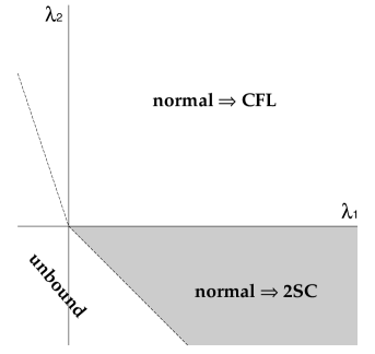
a)          b)

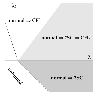
Figure 1: a) Phase diagram of the 3-d GL theory in the coupling constant space obtained by the mean-field theory [2]. The second order phase transitions are obtained. b) Phase diagram obtained by taking into account the gluon fluctuations in a weak-coupling approximation. The phase boundary is shifted and the transition becomes first order.

The mean field approximation to the 3-d GL action leads to the second order transition between normal phase and the color superconducting phase [2]. Fig.1a shows the phase diagram in the ($\lambda_{1}$, $\lambda_{2}$)-plane in the mean field approximation. Whether 2SC or CFL is realized in color superconductor in the chiral limit depends on the sign of $\lambda_{2}$, and the phase boundary is located on $\lambda_{2}=0$.

For weak gauge-coupling, it has been shown that the thermal fluctuation of gauge field dominates over the diquark fluctuation, and can be incorporated as a Gaussian fluctuation around the mean-field [3, 4]. As a result, the phase transition turns into first order, which is similar to the situation in Type I metallic superconductor [5]. Shown in Fig.1b is a phase diagram in the ($\lambda_{1},\lambda_{2}$)-plane obtained by using the weak coupling approximation along the line of ref.[3]. Phase boundary between 2SC and CFL in Fig.1a is shifted towards the positive $\lambda_{2}$ region by the gluon fluctuation. Furthermore, with certain parameter region, we observe successive transitions, normal$\rightarrow$2SC$\rightarrow$CFL, as temperature decreases from above. Since $\lambda_{1}=\lambda_{2}$ is realized in the weak-coupling limit, such successive transitions may take place in high density QCD in the chiral limit. This possibility was first noted in [6].

4 Lattice simulations

Let us discretize the 4-d version of the effective action, Eq.(1), and rescale the field and couplings as $\varPhi\to\sqrt{2\alpha}\varPhi/a$, $\lambda_{i}\to{\bar{\lambda}}_{i}/\alpha^{2}$, $m^{2}\to(1-2\bar{\lambda}_{1}-2{\bar{\lambda}}_{2}-8\bar{\kappa})/\alpha a^{2}$, $\kappa\to\bar{\kappa}/\alpha$ ($a$ being the lattice constant). Then, we reach the following lattice action

$$S=\sum_{x} \left\{{\rm Tr}(\varPhi^{\dagger}_{x}\varPhi_{x})+(\bar{\lambda}_{1}+\bar{\lambda}_{2})\left({\rm Tr}(\varPhi^{\dagger}_{x}\varPhi_{x})-1\right)^{2}+\bar{\lambda}_{2}\left({\rm Tr}(\varPhi^{\dagger}_{x}\varPhi_{x})^{2}-\left[{\rm Tr}(\varPhi^{\dagger}_{x}\varPhi_{x})\right]^{2}\right)\right.$$

$$\ \ -2{\bar{\kappa}}\sum_{\mu}{\rm Re\ Tr}(\varPhi^{\dagger}_{x+\mu}U_{\mu}^{*}\varPhi_{x})+S_{\rm g}(\beta)\Big{\}},$$ (2)

where $S_{\rm g}$ is the standard plaquette action with $\beta\equiv 6/g^{2}$. To ensure that the system is in the deconfined phase, we keep $\beta$ around 5.1 according to the critical value obtained in the pure Yang-Mills case with $N_{\tau}=2$. Taking several sets of the quartic couplings $\bar{\lambda}_{1,2}$, we make simulations by scanning the parameter $\bar{\kappa}$. In this article, we report the results obtained in the simulation with a lattice volume of $2\times 12^{3}$. We note that the $2\times 8^{3}$ lattice gives qualitatively the same results. We use the pseudo heat-bath method to update the gauge-link variables and generalize the efficient update-algorithm of SU(2) Higgs-field [7] to our case.

a)    b)

Figure 2: Eigenvalues of $\sum_{x}\varPhi^{\dagger}_{x}\varPhi_{x}$ as a function of update steps. $(\bar{\lambda}_{1},\bar{\lambda}_{2})=(0.03,0.01)$, $\bar{\kappa}=0.34$, $\beta=5.1$ for the left panel a) and $(\bar{\lambda}_{1},\bar{\lambda}_{2})=(0.03,0.03)$, $\bar{\kappa}=0.43$, $\beta=5.1$ for b). The isolated large eigenvalue associated with two degenerate small eigenvalues a) corresponds to 2SC phase while three degenerate eigenvalues after thermalization b) indicate CFL phase.

The color superconducting phase and the normal phase are distinguished by looking at the gauge invariant operator $\sum_{x}{\rm Tr}\ \varPhi^{\dagger}_{x}\varPhi_{x}$. Although the field fluctuations give non-vanishing expectation value of this operator even in the normal phase, we can observe discontinuous changes of the expectation value as $\bar{\kappa}$ changes. In addition to this, we measure other gauge-invariant operators such as ${\rm Tr}|D_{\mu}\varPhi|^{2},S_{\rm g}$ and the Polyakov loop to confirm that the discontinuous change takes place for all these operators at the same $\bar{\kappa}$. (Note that this discontinuous change of the Polyakov loop does not mean deconfinement transition.) This constitutes an evidence of the first order phase transition.

Moreover, we can differentiate different color superconducting states (2SC, CFL or something else) by diagonalizing the 3$\times$3 matrix $\sum_{x}\varPhi^{\dagger}_{x}\varPhi_{x}$ in the flavor space and extracting its eigenvalues. As shown in Fig.2a, we observe one large eigenvalue with two degenerate small eigenvalues in a particular set of $(\bar{\lambda}_{1},\bar{\lambda}_{2}$). In this case, we regard the state as 2SC in which the quark pairing takes place in one specific color-flavor channel. We also observe three degenerate eigenvalues as shown in Fig.2b with another parameter set, which corresponds to the CFL phase where all channels are involved equally to the pairing. Here we emphasize that this is a gauge invariant way of identifying different phases in color superconductivity. As we scan the parameter $\bar{\kappa}$, we find rapid changes of the eigenvalues of $\sum_{x}\varPhi^{\dagger}_{x}\varPhi_{x}$ at critical value $\bar{\kappa}_{\rm c}$. When we simulate around this point by increasing and decreasing $\bar{\kappa}$, we observe hysteresis loops in the eigenvalues as well as in the Polyakov loop, as shown in Fig.3. Such observation also bears evidence of the first order transition.

Near the critical point of the first order transition, it is always difficult to find a global minimum of the free energy among nearly degenerate local minima. To find a true minimum, we divide the lattice volume into domains so that we can put different phases obtained by the hysteresis loop into different domains. Starting from such a mixed configuration, a state with the highest pressure pushes away the other metastable states after many update steps. We call this as ‘boundary-shift test’. In this way, we can determine the most favorable state for each value of $\bar{\kappa}$ and can estimate $\bar{\kappa}_{\rm c}$.

Figure 3: The hysteresis loop of $\sum_{x}{\rm Tr}\varPhi^{\dagger}_{x}\varPhi_{x}$ obtained by increase or decrease of $\bar{\kappa}$. $(\bar{\lambda}_{1},\bar{\lambda}_{2})=(0.01,0.005)$ and $\beta=5.1$.

In Fig.4, we show the phase diagram in the $(\bar{\lambda}_{1},\bar{\lambda}_{2}$)-plane obtained by our lattice simulations. The points marked by the symbols (star, cross, square, and plus) correspond to the places of actual numerical simulations. We find three types of thermal transitions depending on the coupling parameters: for large values of $\bar{\lambda}_{2}$, transition from the normal phase to CFL takes place as star and cross symbols show. For small or negative values of $\bar{\lambda}_{2}$, transition from the normal phase to 2SC takes place as plus symbols show. In between the two cases, there is a parameter region where successive transition, normal$\rightarrow$2SC$\rightarrow$CFL, takes place as square symbols show.

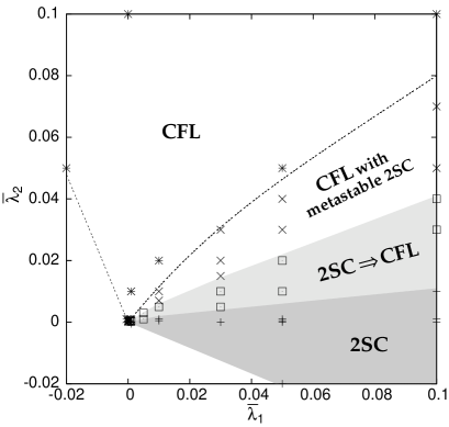
Figure 4: Phase diagram in the coupling constant space obtained by the lattice simulation. Symbols show the parameters at which the actual simulations are carried out.

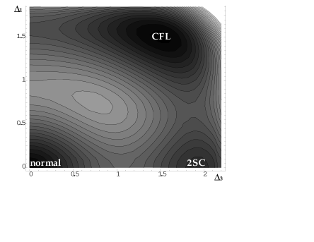
Figure 5: Contour plot of the free energy at the transition point from normal phase to CFL in the weak coupling analysis. Scales are in an arbitrary unit.

The global feature of the phase diagram in Fig.4 is qualitatively similar to that of the weak-coupling analysis shown in Fig.1b, although the coupling constants (e.g. $\lambda_{i}$ vs. $\bar{\lambda}_{i}$) are related in a nontrivial manner. Note that, near the phase boundary between 2SC and CFL, we find a region (shown by the cross symbols) where metastable 2SC survives, even when the global minimum of the free energy transfers directly from the normal phase to CFL. This metastable 2SC state, which is a local minimum of the free energy, can be seen in the hysteresis loop but is pushed away by the ‘boundary-shift test’. The jump of the operators at the transition points becomes smaller if we take larger $\bar{\lambda}_{i}$. It is considered that thermal fluctuations of the diquark field weaken the first order transition.

Fig.5 shows the contour plot of the free energy at a critical point of the transition from the normal phase to the CFL phase obtained in the weak-coupling approach. Setting the diquark field as diag$(\Delta_{1},\Delta_{1},\Delta_{3})$, the gluonic fluctuations are calculated as a function of $\Delta_{1}$ and $\Delta_{3}$. The dark regions have smaller free energy than the light regions. The normal, 2SC and CFL phases are identified as $\Delta_{1}=\Delta_{3}=0$, $(\Delta_{1}=0,\Delta_{3}\neq 0)$ and $\Delta_{1}=\Delta_{3}\neq 0$, respectively. This figure indicates a subtle interplay among three local minima as a function of temperature and coupling constants. It also serves as an possible explanation of the phase structure shown in Fig.4.

5 Discussion

We have studied thermal transitions of color superconductivity on the basis of the lattice simulations of the Ginzburg-Landau effective action. The relevant degrees of freedom are the diquark field $\varPhi$ and the gluon field. We have identified different phases of color superconductivity by measuring the gauge invariant flavor-matrix $\sum_{x}\varPhi^{\dagger}_{x}\varPhi_{x}$ and extracting its eigenvalues. 2SC and CFL phases as well as normal phase are clearly distinguished in a gauge invariant way.

In our simulations, we observed the hysteresis loop of various gauge invariant operators as a function of the parameter $\bar{\kappa}$, which designates the first-order thermal transition. The global minimum of the free energy for each $\bar{\kappa}$ is determined by the boundary-shift method in which we carry out updates by starting from a mixed configuration obtained in the hysteresis loop. With these procedures, we obtained the phase diagram in the coupling constant space and compared the result with that of the weak coupling calculation. Three types of thermal transitions are observed depending on the couplings: normal$\rightarrow$2SC, normal$\rightarrow$CFL and a novel transition, normal$\rightarrow$2SC$\rightarrow$CFL.

To find a realistic phase diagram of color superconductivity in the temperature ($T$) and chemical potential ($\mu$) plane, it is necessary to make a connection of our coupling constants to $T$ and $\mu$, which requires a matching of the GL effective theory to the microscopic QCD. The quark masses and color and charge neutralities become important at low baryon density and will lead to more complex phase structure than that shown in this report. Further studies are needed to attack these problems.

References

-
[1]
K. Rajagopal and F. Wilczek, hep-ph/0011333.
M.G. Alford, Ann. Rev. Nucl. Part. Sci. 51 (2001) 131. - [2] K. Iida and G. Baym, Phys. Rev. D63 (2001) 074018, ibid. D66 (2002) 014015.
- [3] T. Matsuura, K. Iida, T. Hatsuda and G. Baym, Phys. Rev. D69 (2004) 074012.
- [4] I. Giannakis, D. F. Hou, H. C. Ren and D. H. Rischke, Phys. Rev. Lett. 93 (2004) 232301.
- [5] B. I. Halperin, T. C. Lubensky and S. K. Ma, Phys. Rev. Lett. 32 (1974) 292.
- [6] T. Matsuura, K. Iida, M. Tachibana and T. Hatsuda, talk presented at JPS meeting (March, 2005).
- [7] B. Bunk, Nucl. Phys. (Proc. Suppl.) 42 (1995) 566.