Topology with Dynamical Overlap Fermions

Abstract:

We perform dynamical QCD simulations with $n_{f}=2$ overlap fermions by hybrid Monte-Carlo method on $6^{4}$ to $8^{3}\times 16$ lattices. We study the problem of topological sector changing. A new method is proposed which works without topological sector changes. We use this new method to determine the topological susceptibility at various quark masses.

1 Introduction

The overlap operator [1, 2] , gives a theoretically sound solution of the chirality problem on the lattice. It satisfies the Ginsparg-Wilson relation [3, 4], which ensures the exact chiral symmetry at finite lattice spacing [5], moreover the difference in the number of left and right handed zero modes can be taken as a definition of the topological charge ($Q$) which gives the correct result in the continuum limit [6].

However, the numerical implementation of dynamical overlap fermions is still a great challenge today (for early studies with dynamical overlap fermions we refer to [7, 8, 9]). The presence of nested conjugate gradients for the inversion of the Dirac operator makes the simulations considerably slower than simulations with Wilson fermions. Furthermore one has to face the non-continuity of the fermion determinant at the boundary of topological sectors. This additional difficulty can be treated exactly in frame of the Hybrid Monte Carlo (HMC) algorithm by modifying the molecular dynamics trajectory at the boundary [10]. Clearly the crossing rate between different topological sectors is heavily affected by this modification. Inappropriate treatment might confine the system into a certain topological sector which yields an unacceptably large autocorrelation time for $Q$ in the simulation.

A few exploratory studies are already available in QCD with dynamical overlap fermions [11, 10, 12, 13, 14, 15]. All handle the modification of the trajectory at the boundary in a similar style. The original proposal of [10] is modified in [13] in such a way that the acceptance rate is increased. It is shown in [14], that the introduction of several pseudofermion fields which approximate the fermion determinant, can enhance the crossing rate. The relation between the pseudofermionic (over)estimation and rare topological sector changes was pointed out in [15].

In this paper we study the problem of changing topological sectors in the case of the overlap operator with $n_{f}=2$ fermions in dynamical HMC simulations. Sec. 2 will give a short introduction to the sector changing problem for overlap fermions (by summarizing and extending the work of [15]), and answers the question why the present treatment is unlikely to change $Q$. In Sec. 3 a new measurement method of expectation values is proposed, which circumvents the crossing problem entirely by making simulations constrained to fixed topological sectors. In Sec. 4 we present numerical results using the new measurement method. In Sec. 5 conclusions are given.

2 Topological sector changing problem

After introducing pseudofermion fields [17], our partition function reads:

$$Z=\int[dU]e^{-S_{g}}\det H^{2}=\int[dU][d\phi^{\dagger}][d\phi]e^{-S_{g}-\phi^{\dagger}H^{-2}\phi},$$ (1)

where $H$ is the hermitian overlap operator:

$$H=(1-\frac{m}{2m_{0}})H_{0}+\gamma_{5}m,$$ (2)

with $H_{0}$ being the massless hermitian overlap operator:

$$H_{0}=m_{0}[\gamma_{5}+\textrm{sgn}(H_{W})].$$ (3)

Here $H_{W}$ is the standard Wilson operator with negative mass $-m_{0}$. The sgn function in $H_{0}$ causes a Dirac-$\delta$ type singularity in the equation of motion of the momenta of the link variables. The $\delta$-function gives a contribution whenever an eigenvalue $\lambda$ of $H_{W}$ changes sign. This subspace of the configuration space coincide with topological sector boundaries. The reason for this is that in the case of the overlap operator the topological charge is:

$$Q=\frac{1}{2m_{0}}\textrm{Tr}(H_{0})=\frac{1}{2}\sum_{i}\textrm{sgn}(\lambda_{i})$$ (4)

This means, that there are potential walls, non-differentiable steps in the action at the topological sector boundaries. The reflection-refraction method suggested in [10] handles these potential walls correctly. Let’s denote the momenta by $p$ and the normal vector of the topological sector boundary by $n$. According to this method one has to modify the momenta, when arriving at a potential wall:

$$p\rightarrow\left\{\begin{array}[]{ll}p-n\langle n,p\rangle+n\langle n,p\rangle\sqrt{1-2\frac{\Delta S}{\langle n,p\rangle^{2}}},&\textrm{if}\ \langle n,p\rangle^{2}>2\Delta S\ \textrm{(refraction)}\\ p-2n\langle n,p\rangle,&\textrm{if}\ \langle n,p\rangle^{2}<2\Delta S\ \textrm{(reflection)}\end{array}\right.$$ (5)

Thus the trajectory will go through the topological sector boundary only if $\langle n,p\rangle^{2}>2\Delta S$. In a HMC algorithm $\langle n,p\rangle=\mathcal{O}(1)$ and has exponential distribution. $\Delta S$, however, is not the exact value of the height of the potential wall, but it is the change of the pseudofermionic action at the boundary. From now on, we will distinguish between these two quantities. We call the former $\Delta S_{\textrm{exact}}$ and the latter $\Delta S_{\textrm{pf}}$.

Let us take a closer look on the relation between $\Delta S_{\textrm{exact}}$ and $\langle\Delta S_{\textrm{pf}}\rangle$. In particular, we show that the jump in the pseudofermionic action overestimates $\Delta S_{\textrm{exact}}$. Let us assume that the trajectory crosses the boundary. Let $H_{-}$ and $H_{+}$ be the overlap operator evaluated on the two sides of the boundary right before and after the crossing, respectively. Clearly $H_{-}$ and $H_{+}$ contain the same gauge configuration, but they differ, since one eigenvalue of $H_{W}$ changes sign on the boundary. In the HMC algorithm one chooses the pseudofermion field as

$$\phi=H_{-}\eta,\ \ \ \ \ \phi^{\dagger}=\eta^{\dagger}H_{-},$$

where $\eta,\eta^{\dagger}$ are random vectors with Gaussian distribution, in order to generate $\phi,\phi^{\dagger}$ with the correct distribution. (In a real simulation one chooses new pseudofermion configurations only at the beginning of each trajectory, but for simplicity let’s consider, that $\phi$ and $\phi^{\dagger}$ are refreshed when hitting the boundary.) The jump of the pseudofermionic action now reads:

$$\Delta S_{\textrm{pf}}=S_{\textrm{pf}+}-S_{\textrm{pf}-}=\eta^{\dagger}(H_{-}H^{-2}_{+}H_{-}-1)\eta$$

The relation between $\Delta S_{\textrm{exact}}$ and $\Delta S_{\textrm{pf}}$ can be obtained by the following straightforward calculation:

$$e^{-\Delta S_{\textrm{exact}}}=\frac{\det H^{2}_{+}}{\det H^{2}_{-}}=\frac{\int[d\eta^{\dagger}][d\eta]e^{-\eta^{\dagger}\eta}e^{-\eta^{\dagger}(H_{-}H^{-2}_{+}H_{-}-1)\eta}}{\int[d\eta^{\dagger}][d\eta]e^{-\eta^{\dagger}\eta}}=$$

$$=\langle e^{-\eta^{\dagger}(H_{-}H^{-2}_{+}H_{-}-1)\eta}\rangle_{\eta^{\dagger}\eta}\geq e^{-\langle\eta^{\dagger}(H_{-}H^{-2}_{+}H_{-}-1)\eta\rangle_{\eta^{\dagger}\eta}}=e^{-\langle\Delta S_{\textrm{pf}}\rangle}$$

The inequality in the second line is a consequence of the concavity of the $e^{-x}$ function. So we conclude to:

$$\langle\Delta S_{\textrm{pf}}\rangle\geq\Delta S_{\textrm{exact}}.$$

We can examine this relation in realistic simulations, if we take into account, that there is a simple relation between $H_{+}$ and $H_{-}$. Let’s denote by $\lambda_{0}$ the eigenvalue of $H_{W}$ which crosses zero at the boundary, and by $|0\rangle$ the eigenvector belonging to $\lambda_{0}$. With this notation:

$$H_{+}=H_{-}+c|0\rangle\langle 0|,$$

where

$$c=\Delta\textrm{sgn}\lambda_{0}\ m_{0}(1-\frac{m}{2m_{0}}),$$

with $\Delta\textrm{sgn}\lambda_{0}=\pm 2$ being the jump of ${\rm sgn}\lambda_{0}$ on the boundary. The expectation value of the discontinuity in the pseudofermionic action is:

$$\langle\Delta S_{\textrm{pf}}\rangle=\langle\eta^{\dagger}(H_{-}H^{-2}_{+}H_{-}-1)\eta\rangle_{\eta^{\dagger}\eta}=\textrm{Tr}(H_{-}H^{-2}_{+}H_{-}-1)=$$

$$=\textrm{Tr}\big{(}(1-c|0\rangle\langle 0|H_{+}^{-1})(1-c\ H_{+}^{-1}|0\rangle\langle 0|)-1\big{)}=-2c\langle 0|H_{+}^{-1}|0\rangle+c^{2}\langle 0|H_{+}^{-2}|0\rangle.$$ (6)

In a similar way one can get a simple formula for the exact value of the jump on the boundary:

$$e^{-\Delta S_{\textrm{exact}}}=\frac{\det H_{+}^{2}}{\det H_{-}^{2}}=\frac{1}{\det(H_{+}^{-1}H_{-})^{2}}=\frac{1}{\det(1-cH_{+}^{-1}|0\rangle\langle 0|)^{2}}=\frac{1}{(1-c\langle 0|H_{+}^{-1}|0\rangle)^{2}}.$$ (7)

eq. (6) and eq. (7) offers a numerically fast way to determine both action jumps, since one needs only one inversion of the overlap operator to obtain both of them.

Figure 1: The jump in the exact vs. pseudofermionic action at $\beta=4.05$ and $m=0.1,0.2$. Since the average of $\langle n,p\rangle^{2}$ is around $\approx 1$, topological sector changing would happen considerably frequently using $S_{\rm exact}$, than with $S_{\rm pf}$. We also indicated the probability of topological sector changing with the pseudofermionic action, and an estimate on the probability using the exact action (assuming that the two algorithms would behave the same way except for the boundaries).

For illustration we made a scatter plot (Fig. 1) from a $6^{4}$ lattice at two different masses. (Details of our action will be described in Section 4.) One can clearly see, that the use of the pseudofermions has an awkward consequence: there are a huge amount of crossings, where the topological sector changing fails only due to the overestimation. One way to cure this is to use several pseudofermion estimators instead of one [14]. More pseudofermions mean smaller spread of the pseudofermionic action distribution, therefore the overestimation is smaller, too. However the computational time also increases with the number of extra fields. Obviously the best would be to use the exact action in the simulations, but only its discontinuity on the boundary can be calculated easily. The next section will present a technique, which uses this discontinuity to get the relative weight of topological sectors.

3 The new method

In this section we propose a new method for the calculation of physical observables by which it becomes possible to circumvent the problem of topological sector changing described in the previous section. Let us write the partition function in the form (assuming a vanishing $\theta$ parameter):

$$Z=\sum_{Q=-\infty}^{\infty}Z_{Q},$$

where $Z_{Q}$ is the partition function of the topological sector $Q$. The expectation value of an observable:

$$\langle O\rangle=\frac{\sum_{Q}Z_{Q}\langle O\rangle_{Q}}{\sum_{Q}Z_{Q}}=\frac{\sum_{Q}\frac{Z_{Q}}{Z_{0}}\langle O\rangle_{Q}}{\sum_{Q}\frac{Z_{Q}}{Z_{0}}},$$

where the restricted expectation value $\langle O\rangle_{Q}$ is

$$\langle O\rangle_{Q}=\frac{1}{Z_{Q}}\int[dU]_{Q}O[U]\det H^{2}_{Q}\exp(-S_{g}).$$

For reasons which will be clear later the integration goes not only over the configurations with $Q$ charge, but also over the boundary of the topological sector as well (though the boundary has only zero measure in this case). When calculating the partition function in a given topological sector the following boundary prescription is used: we define the determinant on the boundary as the limit of determinants approaching the wall from the $Q$ side ($\det H^{2}_{Q}$). If the measurement of the quantities $Z_{Q+1}/Z_{Q}$ would be possible, then we could recover $Z_{Q}/Z_{0}$ for any $Q$. With these in hand, we would need only the restricted expectation values $\langle O\rangle_{Q}$, whose measurement doesn’t require topological sector changings.

Now we will show a way to measure $Z_{Q+1}/Z_{Q}$. It will make use of the fact, that we can calculate easily $\Delta S_{\textrm{exact}}$ on the boundary of topological sectors (see eq. (7)). The pseudofermionic action is only used to generate configurations in fixed topological sectors, so its bad distribution for the jump of the action will not effect us. (In the following formulae $\Delta S$ will automatically mean $\Delta S_{\textrm{exact}}$.) The main idea is the following: an observable measured in sector $Q$ is inversely proportional to $Z_{Q}$ and an observable in $Q+1$ is to $Z_{Q+1}$. If the observables in the two sectors are concentrated only to the common wall separating the two sectors, then from the ratio of the two expectation values one can recover the ratio of the two sectors.

First let us measure in the $Q$ sector an operator, which is concentrated to the boundary:

$$\langle\delta_{Q,Q+1}F\rangle_{Q}=\frac{1}{Z_{Q}}\int[dU]_{Q}\delta_{Q,Q+1}F[U]\det H^{2}_{Q}\exp(-S_{g}),$$ (8)

where we introduced the distribution $\delta_{Q,Q+1}$, a Dirac-$\delta$, which is equal to zero everywhere but on the $Q,Q+1$ boundary. Then let us measure another operator $G$ on the same wall (thus on the boundary separating sectors $Q$ and $Q+1$), but now from the $Q+1$ sector:

$$\langle\delta_{Q,Q+1}G\rangle_{Q+1}=\frac{1}{Z_{Q+1}}\int[dU]_{Q+1}\delta_{Q,Q+1}G[U]\det H^{2}_{Q+1}\exp(-S_{g}).$$ (9)

The wall is the same (i.e. $[dU]_{Q}\delta_{Q,Q+1}=[dU]_{Q+1}\delta_{Q,Q+1}$) in both cases, however due to our boundary prescription the determinants are different on it. Therefore if $F$ and $G$ satisfies:

$$F[U]\det H^{2}_{Q}[U]=G[U]\det H^{2}_{Q+1}[U],$$ (10)

then the ratio of eq. (8) and eq. (9) gives us

$$\frac{\langle\delta_{Q,Q+1}F\rangle_{Q}}{\langle\delta_{Q,Q+1}G\rangle_{Q+1}}=\frac{Z_{Q+1}}{Z_{Q}}.$$ (11)

The easiest choice is $G(U)=1$ and $F(U)=\det H^{2}_{Q+1}/\det H^{2}_{Q}=\exp(-\Delta S)$, the ratio of sectors becomes:

$$Z_{Q+1}/Z_{Q}=\frac{\langle\delta_{Q,Q+1}\exp(-\Delta S)\rangle_{Q}}{\langle\delta_{Q,Q+1}\rangle_{Q+1}}.$$ (12)

This choice is still not optimal, since the measurement of the numerator is problematic, if the distribution of $\Delta S$ extends to negative values. The exponential function amplifies the small fluctuations in the negative $\Delta S$ region, which can destroy the whole measurement: a very small fraction of the configurations will dominate the result. As a consequence one ends up with relatively large statistical uncertainties. With a slightly different choice of $F$ and $G$ we can improve on the situation. With $F(U)=\Theta(\Delta S-x)\exp(-\Delta S)$ and $G(U)=\Theta(\Delta S-x)$ we can omit the problematic part of the $\Delta S$ distribution (the values smaller than $x$) from the measurement, and we get:

$$Z_{Q+1}/Z_{Q}=\frac{\langle\delta_{Q,Q+1}\exp(-\Delta S)\rangle_{Q}^{\Delta S>x}}{\langle\delta_{Q,Q+1}\rangle_{Q+1}^{\Delta S>x}}.$$ (13)

The price of this choice of $F,G$ is that we do not make use of the $\Delta S<x$ part of our data set. The value of $x$ can be tuned to minimize the statistical error.

Let us note that eq. (10) can be viewed as a detailed balance condition on a given $U$ configuration between $Q$ and $Q+1$ sector ($F$ and $G$ are just the “transition probabilities”). This can give us a hint, that the Metropolis-step is a good a solution for $F,G$: $F=\min(1,\exp(-\Delta S))$ and $G=\min(1,\exp(\Delta S))$. The ratio of sectors is simply:

$$Z_{Q+1}/Z_{Q}=\frac{\langle\delta_{Q,Q+1}\min(1,\exp(-\Delta S))\rangle_{Q}}{\langle\delta_{Q,Q+1}\min(1,\exp(\Delta S))\rangle_{Q+1}}.$$ (14)

The inconvenient part of the distribution ($\Delta S<0$) is cut off, however in contrast to eq. (13) all configurations are used to get the expectation values.

We have achieved our main goal: without making expensive topological sector changes we can obtain the ratio of sectors (see eq. (12, 13, 14)). The key point is to make simulations constrained to fixed topological charge, and match the results on the common boundaries of the sectors. In the next subsection we will show in the framework of HMC, how to measure an expectation value, which contains a Dirac-delta on the surface. Our proposal is that the generation of trajectories inside a sector can be done using the pseudofermionic action, we do not need there the exact action. Since no sector changing is required, the inconvenient distribution of the pseudofermionic action jump on the boundary will not effect the measurement of the ratios of sectors. The exact action is needed only on the boundary: the formulas (12, 13, 14) require $\Delta S$.

It is clear that using the exact fermion action when measuring the ratio of sectors outperforms the conventional HMC, where topological sector changing is hindered by the distribution of the pseudofermionic action jump. Even in that (at the moment theoretical) case if we were able to use the exact fermionic action in simulations, the above presented method is better in determining the ratios of topological sectors. Consider a small quark mass simulation, where a HMC using the exact fermionic action sticks into the trivial topological sector (now due to the fact, that nontrivial topologies are suppressed by the fermion determinant). If the simulation time is not long enough, then we have no information at all on the small (but nonvanishing) ratio $Z_{1}/Z_{0}$. However in our method this small quantity can be measured. The more we hit the wall from the two sides the more precisely we can measure $Z_{1}/Z_{0}$. The same argument applies to an R-type algorithm (where it is possible to use the exact $\Delta S$ jump, when crossing topological sectors [15]).

Obviously an important issue for this new method is whether topological sectors defined by the overlap charge are path-connected or not. We refer to some results in the Abelian and in the non-Abelian gauge group case [18, 19]. If configurations with the same $Q$ would not be continuously connectable in sector $Q$, then our assumption that we make measurements on the common boundary of sectors could be violated. It could happen, that the wall sampled from sector $Q$ does not coincide with the wall sampled from $Q+1$. Moreover the fixed sector simulations would also violate ergodicity in this case. Let us note here that the large autocorrelation time for the topological charge in the conventional pseudofermionic HMC effectively also causes the breakdown of ergodicity. In case of non-connected sectors one can cure these problems by releasing the system from a sector after a certain amount of time and closing it to another.

Expectation value of a $\delta$-function

In a HMC simulation one determines the expectation value of an operator by calculating a sum over the measured values of the observable on $N$ configurations, which are generated with the proper weights, by which they occur in the functional integral. In practice it is not possible to measure an operator containing a Dirac-delta on the boundary surface on these configurations, because none of them will be exactly located on it. Therefore we formulate a somewhat different measurement method, and discuss its properties. As a result one has to make measurements at those points of the trajectories, where they hit the boundary.

Let us see the details. Consider for a moment that we are able to integrate the Hamiltonian equations of motion exactly. If the distribution of the gauge field, pseudofermion field and momenta was correct at the starting point of the trajectory, then it will be still correct for any of the inner points. This fact follows from energy and area conservation and reversibility. So we make no mistake if we put the inner points of the trajectory into the ensemble. We can write:

$$\langle O\rangle=\lim_{N\to\infty}\frac{1}{N}\sum_{i=1}^{N}O_{i}=\lim_{N\to\infty}\frac{1}{N}\sum_{i=1}^{N}\int_{i}O(U_{t})dt=\lim_{N\to\infty}\frac{1}{N}\sum_{i=1}^{N}O_{i,i+1}$$ (15)

where $t$ is the microcanonical time, $U_{t}$ is the gauge configuration at time $t$, the $i$ subscript at the integral means that the integration goes for the $i$th trajectory, and $O_{i,i+1}$ is thus the average of the operator $O$ along this trajectory. In the case of an observable, which contains a $\delta$-function, like those in eq. (13) or in eq. (14) this reads:

$$O_{i,i+1}=\int_{i}dt\ o(U_{t})\ \delta\left(\lambda_{0}(U_{t})\right),$$ (16)

where it is indicated, that the $\delta$-function depends on the gauge configuration only through the smallest absolute value eigenvalue $\lambda_{0}$ of $H_{W}$. If the variable of integration is changed from $t$ to $\lambda_{0}$, we get:

$$O_{i,i+1}=\int d\lambda_{0}\sum_{j}\left|\frac{dt}{d\lambda_{0}}\right|_{t_{j},\lambda_{0}(U_{t_{j}})=0}o(U_{t_{j}})\delta(\lambda_{0}).$$ (17)

We can go further by determining the time derivative of the smallest eigenvalue:

$$\frac{d\lambda_{0}}{dt}=\langle 0|\textrm{tr}\frac{\partial H_{W}}{\partial U^{T}}\frac{dU}{dt}|0\rangle$$ (18)

where, again $|0\rangle$ is the eigenvector belonging to $\lambda_{0}$. The trace and transpose operations are meant to be in color space. Recognizing, that with our previous notation

$$\frac{dU}{dt}=pU\ \ \ \textrm{and}\ \ \ \langle 0|U\frac{\partial H_{W}}{\partial U^{T}}|0\rangle=n$$

yields

$$\frac{d\lambda_{0}}{dt}=\langle n,p\rangle,\ \ \ \left|\frac{dt}{d\lambda_{0}}\right|=\frac{1}{|\langle n,p\rangle|},$$ (19)

$$\langle O\rangle=\lim_{N\to\infty}\frac{1}{N}\sum_{i=1}^{N}\sum_{j}\left.o(U_{t_{j}})\frac{1}{|\langle n,p_{t_{j}}\rangle|}\right|_{t_{j},\lambda_{0}(U_{t_{j}})=0}$$ (20)

If we put it simple, the above formula says, that since the integration is in microcanonical time, the angle and velocity by which the trajectory hits the boundary has to be taken into account.

Let us turn back to the case, when the integration of the equations of motion can be done only with finite step size integrator. The leap-frog procedure has $O(\epsilon^{3})$ error per microcanonical step, which after $1/\epsilon$ steps makes the trajectory differ by $O(\epsilon^{2})$ from the exact trajectory. If we can guarantee, that the modification of the trajectory at the boundary also violates the equations of motions only upto $O(\epsilon^{2})$, then in the final results the errors will be proportional with $O(\sqrt{N}\epsilon^{2})$. The original reflection algorithm in [10] has $O(\epsilon)$ errors, later it was improved to $O(\epsilon^{2})$ in [13]. In the Appendix we propose a different reflection procedure and prove that it is reversible, area-preserving and conserves the energy upto $O(\epsilon^{2})$.

4 Numerical results

In the previous section we described a new method, to solve the topological sector changing problem of pseudofermionic HMC simulation. We describe here the details of the simulations, and finally give the topological susceptibility in physical units measured on $8^{4}$ and $8^{3}\times 16$ lattices.

Simulations were done using unit length trajectories, separated by momentum and pseudofermion refreshments. The system was confined to a fixed topological sector in each run, we reflected the trajectories whenever they reached a sector boundary. The end points of the trajectories obviously follow the exact distribution in a given sector, usual quantities can be measured on them. When calculating the ratio of sectors using eq. (12) or eq. (13) or eq. (14) we integrated along the trajectories, this quantity will be burdened by a step size error.

Figure 2: Left panel: a typical optimization procedure of the lower limit ($x$) on $\Delta S$ in the formula (13). The statistical error of the ratio $Z_{1}/Z_{0}$ shows a minimum as the function of $x$, which is considered as the optimal value. Right panel: Bare mass dependence of topological susceptibility using three different methods on $6^{4}$ lattices. The points corresponding to the same mass were slightly shifted vertically for clarity. Result based on our new technique and eq. (13) is on the left, based on eq. (14) is in the middle, the standard pseudofermionic HMC is on the right. The simulation parameters are from [20]

In case of large enough statistics the value of $Z_{Q+1}/Z_{Q}$ should be the same, independently which of the three formula (12, 13, 14) was used to calculate it. We omit eq. (12) in the following, since it is hard to give a reliable error estimate on the expectation value of $\exp(-\Delta S)$, if $\Delta S$ can be arbitrary negative number. Eq. (13) still measures $\exp(-\Delta S)$, but with a lower limit ($x$) on $\Delta S$. Smaller limit yields a smaller and more reliable error, however the statistics is decreased at the same time. One can tune the value of $x$, so that the statistical error takes its minimum. A result of a typical optimum search can be seen on the left panel of Fig. 2. The optimal value can be compared to the one obtained from eq. (14). On the right panel of Fig. 2 the two new topological susceptibilities and the one calculated by using traditional pseudofermionic HMC [20] are shown. The agreement is perfect.

m	$r_{0}$	$m_{\pi}$	$Lm_{\pi}$
$0.03$	$3.52(13)$	$0.29(11)$	$2.4$
$0.1$	$3.17(5)$	$0.53(4)$	$4.3$
$0.2$	$2.89(2)$	$0.74(6)$	$5.9$
$0.3$	$2.88(6)$	$0.99(8)$	$7.9$

Table 1: Sommer-scale, pion mass and pion mass times box size on $8^{3}\times 16$ lattices.

To measure the topological susceptibility on $8^{4}$ lattices we generated configurations with tree-level Symanzik improved gauge action ($\beta=4.15$ gauge coupling) and 2 step stout smeared overlap kernel ($\rho=0.15$ smearing parameter, the kernel was the standard Wilson matrix with $m_{0}=1.3$). We performed runs in sectors $Q=0\dots 3$ (based on the measured $Z_{3}/Z_{2}$ we can conclude, that the contribution of $Q\geq 4$ sectors are small compared to statistical uncertainties). For the negatively charged sectors we used the $Q\to-Q$ symmetry of the partition function. The bare masses were $m=0.03,0.1,0.2$ and $0.3$, at each mass approximately 1000 trajectories were collected. The average number of the topological sector boundary hittings was around $1.5$ per trajectory. We calculated the ratio of sectors using eq. (13) and eq. (14). The result for the topological susceptibility can be seen on Fig. 3. It is nicely suppressed for the smallest mass. To convert it into physical units, we measured the static potential and the pion mass on $8^{3}\times 16$ lattices (Table 1). Since our statistics was quite small on these asymmetric lattices, the errors are large. Note, that in order to get the mass-dimension 4 topological susceptibility in physical units, one has to make very precise scale measurements.

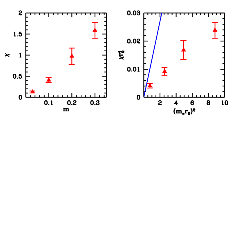
Figure 3: Topological susceptibility as the function of quark mass on $8^{4}$ lattices in lattice units (left), and in physical units as the function of pion mass (right). Scale fixing and mass measurements were done on $8^{3}\times 16$. The error bars on the right plot do not contain the errors of scale fixing. The line is the leading order chiral behavior in the continuum.

When interpreting the results, one should keep in mind, that the volume is small, and the lattice spacing is large. Note however, that smeared kernel overlap actions show nice scaling behavior and good locality properties already at moderate lattice spacings[21, 22].

5 Conclusions

In this paper we studied the problem of topological sector changing in dynamical overlap simulations. The origin of the unexpectedly large autocorrelation time for the topological charge is connected to pseudofermions, which approximate the fermion determinant. The pseudofermionic action overestimates the size of the discontinuity in the fermion determinant at the topological sector boundary, so the system cannot enter easily to a new topological sector. This happens even if the use of the exact determinant favored a transition. (The discontinuity of the exact determinant can be calculated in a rather inexpensive way.)

We developed a new method, which circumvents the problem of topological sector changing. It confines the system to fixed topological sectors (by always reflecting the HMC trajectories from the topological sector boundaries). Thus overestimating the discontinuity of the determinant due to pseudofermions will not effect the determination of topology related quantities. The relative weight of two topological sector is obtained by measuring appropriate operators on the common boundary surface. The measurement of such operators can be carried out by extending the usual HMC measurement method, however an $O(\epsilon^{2})$ extrapolation in HMC step size is required.

The new method was tested on $6^{4}$ lattices, where previous conventional HMC results were available. The old and new results were consistent. We also measured the topological susceptibility on $8^{4}$ lattices with an improved overlap fermion and gauge action, furthermore simulations were done on $8^{3}\times 16$ lattices to convert the lattice results into physical units.

Acknowledgments:
Useful comments on the manuscript from A. D. Kennedy and discussions with T. G. Kovács are acknowledged. For this work a modified version of the MILC Collaboration’s public code [23] with SSE instructions [24] was used. Simulations were carried out on the ALICENext PC-Cluster (1024 AMD-Opteron processors) at Wuppertal University, Germany and on the PC-cluster (330 Intel-P4 nodes) at the Eötvös University of Budapest, Hungary. This work was partially supported by Hungarian Scientific grants, OTKA-T34980/T37615/M37071/T032501/AT049652. This research is part of the EU Integrated Infrastructure Initiative Hadronphyisics project under contract number RII3-CT-20040506078.

Appendix

We present a reflection algorithm which conserves the energy upto $O(\epsilon^{2})$, and which is reversible and area conserving. Until the boundary the trajectory is evolved by the usual leapfrog procedure. An elementary leapfrog step can be written in the following symbolic way:

$$P(\epsilon/2)U(\epsilon)P(\epsilon/2),$$ (21)

where $U(\epsilon)$ and $P(\epsilon)$ are the operators updating the links ($u$) and the momenta ($p$):

$$U(\epsilon):u\to\exp(\epsilon p)u, P(\epsilon):p\to p-\epsilon A\left[u\frac{\partial}{\partial u}\left(S_{g}+S_{\rm pf}\right)\right],$$

where in the force term the $A$ operator projects onto traceless, antihermitian matrices (in color indices). Now we split the evolution of the links into two parts:

$$P(\epsilon/2)U(\epsilon/2)\cdot U(\epsilon/2)P(\epsilon/2).$$ (22)

Consider that the boundary would be crossed during one of the evolutions of the links in eq. (22). Then replace the original leapfrog with the following:

$$P(\epsilon/2)U(\epsilon/2)\cdot U(\epsilon_{c})P(\epsilon_{c})RP(\epsilon_{c})U(\epsilon_{c})\cdot U(\epsilon/2)P(\epsilon/2),$$

where $R$ is simply the reflection of the momenta (eq. (5)). $\epsilon_{c}$ is the time to reach the boundary surface measured from the midpoint of the leapfrog. Thus if the crossing would happen in the first evolution then $\epsilon_{c}<0$, if in the second, then $\epsilon_{c}>0$. The reversibility can be checked easily, for the energy conservation we note that both $U(\epsilon)P(\epsilon)$ and $P(\epsilon)U(\epsilon)$ conserves the energy upto $O(\epsilon^{2})$. If the evolution time does not depend on the variables, then both $U(\epsilon)$ and $P(\epsilon)$ are area conserving. The only problem arises due to the link and momenta dependence of $\epsilon_{c}$. We will now show that the combined effect of the $\epsilon_{c}$ updates

$$U(\epsilon_{c})P(\epsilon_{c})RP(\epsilon_{c})U(\epsilon_{c})$$ (23)

is still area preserving.

For simplicity we will not carry out here the computation using the $SU(3)$ structure, but only for a $k$-dimensional Euclidean vectorspace (the $q$ coordinates are $k$-component vectors). All features of the proof are also present in this simpler case. We have to calculate the Jacobian of the following transformation

$$q^{\prime}(q,p)=q+\epsilon_{c}p+\epsilon_{c}p^{\prime} p^{\prime}(q,p)=Rp+h.$$

$R_{ab}=\delta_{ab}-2n_{a}n_{b}$ is the reflection operator ($a,b=1\dots k$), where $n_{a}$ is the normal vector of the surface. $h$ can be expressed as $h=-\epsilon_{c}F-\epsilon_{c}RF$, where $F$ is the force on the wall (interpreted in the sector into which we reflect back the trajectory). Since $h$ is measured on the wall, its $q$ and $p$ derivatives satisfy $\partial h/\partial p=\epsilon_{c}\partial h/\partial q$ (see [10]). Furthermore $h$ is orthogonal to $n$ ($(nh)=0$). For the $q$ derivative of $p^{\prime}$ we introduce the matrix $Z_{ab}$, which contains the derivatives of the normal vector and $h$:

$$\frac{\partial p^{\prime}_{a}}{\partial q_{b}}=Z_{ab}.$$

Using that $n$ and $h$ are functions of the wall coordinates, $\epsilon_{c}Z$ will appear in the $p$ derivative of $p^{\prime}$:

$$\frac{\partial p^{\prime}_{a}}{\partial p_{b}}=R_{ab}+\epsilon_{c}Z_{ab}.$$

The partial derivatives of $q^{\prime}$ are:

$$\frac{\partial q^{\prime}_{a}}{\partial q_{b}}=\delta_{ab}+(p_{a}+p^{\prime}_{a})\frac{\partial\epsilon_{c}}{\partial q_{b}}+\epsilon_{c}\frac{\partial p^{\prime}_{a}}{\partial q_{b}},$$

$$\frac{\partial q^{\prime}_{a}}{\partial p_{b}}=\epsilon_{c}\delta_{ab}+(p_{a}+p^{\prime}_{a})\frac{\partial\epsilon_{c}}{\partial p_{b}}+\epsilon_{c}\frac{\partial p^{\prime}_{a}}{\partial p_{b}}.$$

With the help of the following identities (see [10]):

$$\frac{\partial\epsilon_{c}}{\partial q_{a}}=-\frac{n_{a}}{(np)} \frac{\partial\epsilon_{c}}{\partial p_{a}}=-\epsilon_{c}\frac{n_{a}}{(np)},$$

the Jacobian can be written in a hypermatrix form (${x\circ y}$ has components $x_{a}y_{b}$):

$$J=\begin{pmatrix}\frac{\partial q^{\prime}}{\partial q}&\frac{\partial q^{\prime}}{\partial p}\\ \frac{\partial p^{\prime}}{\partial q}&\frac{\partial p^{\prime}}{\partial p}\\ \end{pmatrix}=\begin{pmatrix}{1}&-2\epsilon_{c}{Q}\\ {0}&{R}\end{pmatrix}-\frac{1}{(np)}\begin{pmatrix}1&\epsilon_{c}\\ 0&0\end{pmatrix}\otimes[(p+p^{\prime})\circ n]+\begin{pmatrix}\epsilon_{c}&\epsilon_{c}^{2}\\ 1&\epsilon_{c}\end{pmatrix}\otimes{Z}.$$

$Q$ is the projector to the subspace orthogonal to $n$ ($Q=1-n\circ n$). $J$ can be written as a product of two matrices $J=J_{1}J_{2}$, where

$$J_{1}=\begin{pmatrix}{1}&-2\epsilon_{c}{Q}\\ {0}&{R}\end{pmatrix},$$

having determinant $-1$ (since $R$ is a reflection).

$$J_{2}=\begin{pmatrix}1&0\\ 0&1\end{pmatrix}\otimes{1}-\frac{1}{(np)}\begin{pmatrix}1&\epsilon_{c}\\ 0&0\end{pmatrix}\otimes[(p+p^{\prime})\circ n]+\begin{pmatrix}-\epsilon_{c}&-\epsilon_{c}^{2}\\ 1&\epsilon_{c}\end{pmatrix}\otimes{RZ},$$

which has an upper triangular form in the $2\times 2$ space in a suitable basis. The determinant of $J_{2}$ will be unity due to the orthogonality of $p+p^{\prime}=p+Rp+h=-2Qp+h$ and $n$. Therefore $\det J=-1$, which shows that the transformation (23) preserves the area.

References

- [1] H. Neuberger, Phys. Lett. B 417 (1998) 141 [arXiv:hep-lat/9707022].
- [2] H. Neuberger, Phys. Lett. B 427 (1998) 353 [arXiv:hep-lat/9801031].
- [3] P. H. Ginsparg and K. G. Wilson, Phys. Rev. D 25, 2649 (1982).
- [4] P. Hasenfratz, Nucl. Phys. Proc. Suppl. 63 (1998) 53 [arXiv:hep-lat/9709110].
- [5] M. Luscher, Phys. Lett. B 428 (1998) 342 [arXiv:hep-lat/9802011].
- [6] P. Hasenfratz, V. Laliena and F. Niedermayer, Phys. Lett. B 427, 125 (1998) [arXiv:hep-lat/9801021].
- [7] R. Narayanan, H. Neuberger and P. M. Vranas, Phys. Lett. B 353, 507 (1995) [arXiv:hep-lat/9503013].
- [8] H. Neuberger, Phys. Rev. D 60 (1999) 065006 [arXiv:hep-lat/9901003].
- [9] A. Bode, U. M. Heller, R. G. Edwards and R. Narayanan, arXiv:hep-lat/9912043.
- [10] Z. Fodor, S. D. Katz and K. K. Szabo, JHEP 0408, 003 (2004) [arXiv:hep-lat/0311010].
- [11] G. Arnold, N. Cundy, J. van den Eshof, A. Frommer, S. Krieg, T. Lippert and K. Schafer, arXiv:hep-lat/0311025.
- [12] N. Cundy, J. van den Eshof, A. Frommer, S. Krieg, T. Lippert and K. Schafer, arXiv:hep-lat/0405003.
- [13] N. Cundy, S. Krieg, G. Arnold, A. Frommer, T. Lippert and K. Schilling, arXiv:hep-lat/0502007.
- [14] T. DeGrand and S. Schaefer, Phys. Rev. D 71 (2005) 034507 [arXiv:hep-lat/0412005].
- [15] T. DeGrand and S. Schaefer, Phys. Rev. D 72 (2005) 054503 [arXiv:hep-lat/0506021].
- [16] H. Dilger, Int. J. Mod. Phys. C 6 (1995) 123 [arXiv:hep-lat/9408017].
- [17] S. Duane, A. D. Kennedy, B. J. Pendleton and D. Roweth, Phys. Lett. B 195, 216 (1987).
- [18] M. Luscher, Nucl. Phys. B 549 (1999) 295 [arXiv:hep-lat/9811032].
- [19] D. H. Adams, Nucl. Phys. B 640 (2002) 435 [arXiv:hep-lat/0203014].
- [20] Z. Fodor, S. D. Katz and K. K. Szabo, Nucl. Phys. B (Proc. Suppl.) 140 (2005) 704 [arXiv:hep-lat/0409070].
- [21] T. G. Kovacs, Phys. Rev. D 67, 094501 (2003) [arXiv:hep-lat/0209125].
- [22] S. Durr, C. Hoelbling and U. Wenger, arXiv:hep-lat/0506027.
- [23] http://physics.indiana.edu/~sg/milc.html
- [24] Z. Fodor, S. D. Katz and G. Papp, Comput. Phys. Commun. 152, 121 (2003) [arXiv:hep-lat/0202030].