Topology conserving gauge action and the overlap-Dirac operator

Abstract

We apply the topology conserving gauge action proposed by Lüscher to the four-dimensional lattice QCD simulation in the quenched approximation. With this gauge action the topological charge is stabilized along the hybrid Monte Carlo updates compared to the standard Wilson gauge action. The quark potential and renormalized coupling constant are in good agreement with the results obtained with the Wilson gauge action. We also investigate the low-lying eigenvalue distribution of the hermitian Wilson-Dirac operator, which is relevant for the construction of the overlap-Dirac operator.

I Introduction

Chiral symmetry and topology are tightly related with each other in the gauge field theory through the quantum correction. Namely, the axial anomaly appears at the one-loop level, and its integral over space-time leads to the topological charge of the background gauge field. In principle, one should be able to analyze the implication of this relation for physical observables, such as the neutron electric dipole moment, using the lattice gauge theory, which provides a rigorous formulation of the non-Abelian gauge theories even in the non-perturbative regime. Such study is very difficult with the Wilson-type Dirac operator, since the chiral symmetry is explicitly violated on the lattice.

The overlap-Dirac operator Neuberger:1997fp ; Neuberger:1998wv

$$D=\frac{1}{\bar{a}}\left[1+\gamma_{5}\mathrm{sgn}(aH_{W})\right],\;\;\;\bar{a}=\frac{a}{1+s},$$ (1)

realizes the exact chiral symmetry at finite lattice spacing $a$ Luscher:1998pq satisfying the Ginsparg-Wilson relation Ginsparg:1981bj

$$\gamma_{5}D+D\gamma_{5}=aD\gamma_{5}D.$$ (2)

It is constructed from the Wilson-Dirac operator $aD_{W}$ with the Wilson parameter $r=1$; the hermitian Wilson-Dirac operator $aH_{W}=\gamma_{5}(aD_{W}-1-s)$ enters as an argument of the sign function $\mathrm{sgn}(x)$. The parameter $s$ in (1) is a fixed number in the region $|s|<1$.

Since the definition (1) contains a non-smooth function, the locality of the Dirac operator could be lost when there are near-zero eigenvalues of $|aH_{W}|$. This is consistent with the index theorem, because the index of the Dirac operator, which may be considered as a definition of the topological charge, is a non-smooth function of the background gauge field. When the topological charge changes the value, the Dirac operator must become ill-defined, and this is exactly the point where $aH_{W}$ has a zero eigenvalue.

The locality of the overlap-Dirac operator (1) is guaranteed for the gauge fields on which the minimum eigenvalue of $|aH_{W}|$ is bounded from below by a positive (non-zero) constant Hernandez:1998et . This condition is proved to be satisfied if the gauge field configuration is smooth and each plaquette is close enough to one;

$$||1-P_{\mu\nu}(x)||<\epsilon\;\;\;\;\mbox{for all $x$, $(\mu,\nu)$}.$$ (3)

Here, $P_{\mu\nu}(x)$ is the plaquette variable at $x$ on the $\mu$-$\nu$ plane, and $||\cdots||$ denotes the norm of the operator. In the four-dimensional case, the parameter $\epsilon\simeq 1/20.49$ is a sufficient (but not a necessary) condition Neuberger:1999pz . This is called the “admissibility” bound.

One can construct a gauge action, which generates gauge configurations respecting the condition (3). For instance, Lüscher proposed the action Luscher:1998du

$$S_{G}=\left\{\begin{array}[]{ll}\displaystyle\beta\sum_{P}\frac{1-\mbox{ReTr}P_{\mu\nu}(x)/3}{1-(1-\mbox{ReTr}P_{\mu\nu}(x)/3)/\epsilon},&\;\;\;\mbox{when}\;\;1-\mbox{ReTr}P_{\mu\nu}(x)/3<\epsilon,\\ \infty&\;\;\;\mbox{otherwise}\end{array}\right.,$$ (4)

which has the same continuum limit as the standard Wilson gauge action does. In fact, the limit $\epsilon=\infty$ corresponds to the standard Wilson gauge action. Unfortunately, the bound $\epsilon\simeq 1/20.49$ is too tight to produce gauge field ensembles corresponding to the lattice spacing around 0.1 fm; for practical purposes, one must choose much larger values of $\epsilon$. An interesting question is, then, whether the action can keep the good properties for $\epsilon$ significantly larger than $1/20.49$. To be explicit, one expects that (i) the topology change during the molecular-dynamics-type simulation is suppressed, and (ii) the appearance of the near-zero eigenvalue of $|aH_{W}|$ is suppressed, compared to the standard Wilson gauge action. The point (i) is important in order to efficiently generate gauge configurations with large topological charge, which is necessary for the study of the $\epsilon$-regime or the $\theta$-vacuum. With the point (ii), the locality of the overlap-Dirac operator is improved, and the numerical cost to apply the overlap-Dirac operator is reduced. In the numerical application to the massive Schwinger model with $\epsilon=1$, the stability of the topological charge and the improvement of the chiral symmetry with the domain-wall fermion were observed Fukaya:2003ph ; Fukaya:2004kp . Also, in the four-dimensional quenched QCD, good stability of the topological charge has been reported Shcheredin:2004xa ; Bietenholz:2004mq ; Shcheredin:2005ma ; Nagai:2005fz .

For gauge actions to be useful in practical simulations, good scaling property toward the continuum limit is required. The action (4) differs from the standard Wilson gauge action only at $O(a^{4})$, and we expect that it approaches to the continuum limit as quickly as the standard action does. The scaling would be better for the improved gauge actions, such as the Lüscher-Weisz Luscher:1985zq , Iwasaki Iwasaki:1985we or DBW2 deForcrand:1999bi gauge actions, but an advantage of (4) is that it contains a parameter which directly controls the admissibility bound and thus the appearance of the low-lying modes of $aH_{W}$. For the improved actions including the rectangle loop, on the other hand, the low-lying modes are suppressed for large values of the rectangle coupling (e.g. with the DBW2 action) at the price of loosing the good scaling for short distance quantities DeGrand:2002vu .

The goal of this paper is to give a systematic quenched QCD study of the topology conserving gauge action. We find that the topology change is indeed suppressed when the parameter $\epsilon$ is of order one. We also find that the scaling violation in the static quark potential remain reasonably small and the tadpole improved perturbation theory for the renormalized gauge coupling shows a good convergence in the parameter range of our study. Therefore, the topology conserving gauge action has a desired properties for a practical application. Here we would like to comment on the possible application for the future work with the dynamical overlap fermion. In the standard method, with the Wilson plaquette action, one projects out the smallest eigenmodes of $H_{W}$ at every molecular dynamics step in the simulation trajectory and judge if the topology change occurs or not. When the topology change occurs, one recalculates the link updation with much higher accuracy on the topology crossing point to choose either entering the new sector (refraction) or going back to the previous sector (reflection) Fodor:2003bh . If one omits this step it would make the acceptance very low due to the non-smoothness of the determinant as a functional of the gauge configuration. On the other hand, if one uses the topology conserving action, crossing $H_{W}=0$ can be strongly suppressed, so that one can avoid the CPU time consuming reflection/refraction method. In this sense, the use of the topology conserving gauge action can also be useful in full QCD simulations with the overlap fermions. Combination with the stout link version of the overlap fermion Morningstar:2003gk would be interesting as well.

This paper is organized as follows. After describing the simulation methods in Section II, we show the fundamental scaling studies in Section III, that is the determination of the lattice spacing and a scaling test with the static quark potential. Renormalization of the coupling constant with the action (4) can be estimated using perturbation theory as described in Section IV. Section V is the main part of this paper; we report how much the topology change may occur with different choices of parameters. In Section VI the locality and the numerical costs of the overlap fermion with gauge fields satisfying the bound (3) are discussed. Conclusion and outlook are given in Section VII.

II Lattice simulations

Although several types of the gauge action that generate the “admissible” gauge fields satisfying the bound (3) are proposed Shcheredin:2004xa ; Bietenholz:2004mq , we take the simplest choice (4). We study three values of $1/\epsilon$: 1, 2/3, and 0. Note that $1/\epsilon=0$ corresponds to the conventional Wilson gauge action. The value $1/\epsilon=2/3$ is the boundary, below this value the gauge links can take any value in the gauge group $SU(3)$ and the positivity is guaranteed Creutz:2004ir .

The link variables are generated with the standard hybrid Monte Carlo algorithm Duane:1987de . We take the molecular dynamics step size $\Delta\tau$ in the range 0.01–0.02 and the number of steps in an unit trajectory $N_{mds}$ = 20–40. During the molecular dynamics steps we monitor that the condition $1-\mbox{ReTr}P_{\mu\nu}(x)/3<\epsilon$ is always satisfied with our choice of the step size. We discarded at least 2000 trajectories for thermalization before measuring observables.

In order to measure the topological charge, we develop a new type of cooling method. It consists of the hybrid Monte Carlo simulation with an exponentially increasing $\beta$ value $\beta_{\mathrm{cool}}$ and decreasing step size $\Delta\tau_{\mathrm{cool}}$ as a function of trajectory $n_{t}$, i.e.

$$\beta_{\mathrm{cool}} = \beta_{\mathrm{init}}\times(1.5)^{n_{t}},$$

$$\Delta\tau_{\mathrm{cool}} = \Delta\tau_{\mathrm{init}}\times(1.5)^{-n_{t}/2},$$ (5)

with a fixed $1/\epsilon_{\mathrm{cool}}$. Note that $\sqrt{\beta_{\mathrm{cool}}}\Delta\tau_{\mathrm{cool}}$ is fixed so that the evolution at each step is kept small. This method allows us to “cool” the configuration smoothly, keeping the admissibility bound (3) with $1/\epsilon=1/\epsilon_{\mathrm{cool}}$. For the parameters, we take $(\beta_{\mathrm{init}},\Delta\tau_{\mathrm{init}},1/\epsilon_{\mathrm{cool}})$ = (2.0, 0.01, 1) for the configurations generated with $1/\epsilon=1$, and (3.5, 0.01, 2/3) for the configurations with $1/\epsilon=2/3$ or $1/\epsilon=0$. Even for the gauge configuration generated with the standard gauge action ($1/\epsilon=0$), the condition $1/\epsilon_{\mathrm{cool}}=2/3$ can be used because it allows all values of SU(3). After 50–200 steps, the link variables are cooled down close to a classical solution in each topological sector. In fact, the geometrical definition of the topological charge Hoek:1986nd

$$Q_{geo}\equiv\frac{1}{32\pi^{2}}\sum_{x}\epsilon^{\mu\nu\rho\sigma}\mbox{ReTr}\left(P_{\mu\nu}(x)P_{\rho\sigma}(x)\right)$$ (6)

of these “cooled” configurations gives numbers close to an integer times a universal factor $Z_{geo}^{-1}$. Namely, $Q=Z_{geo}Q_{geo}$ is close to an integer. We determine $Z_{geo}$ through would-be $Q=1$ gauge configurations, as $Z_{geo}^{-1}$ = 0.923(4). As Figure 1 shows, the topological charge $Q$ is consistent with the index of the overlap-Dirac operator with $s$ = 0.6, which is calculated as described in Section VI. The consistency is better for $1/\epsilon=1$ than for the standard Wilson gauge action $1/\epsilon=0$.

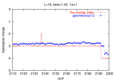
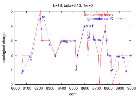
Figure 1: Comparison of the topological charge $Q$, calculated from the geometrical definition $Q_{geo}$ (6) as $Q=Z_{geo}Q_{geo}$, with the index of the overlap-Dirac operator. $Q_{geo}$ is obtained by the cooling method (stars), and the index (pluses) is calculated for the overlap-Dirac operator with $s=0.6$. The agreement is better for $1/\epsilon=1$ (left) than for $1/\epsilon=0$ (right).

To generate topologically non-trivial gauge configurations, we start the hybrid Monte Carlo simulation with the initial condition

$$U_{1}(x)=\left(\begin{array}[]{l}e^{2\pi ix_{4}Q/L^{2}}\\ \;\;\;\;\;\;\;\;1\\ \;\;\;\;\;\;\;\;\;\;\;\;\;e^{-2\pi ix_{4}Q/L^{2}}\end{array}\right), U_{2}(x)=\left(\begin{array}[]{l}1\\ \;\;\;\;\;\;\;\;e^{2\pi ix_{3}\delta_{x_{2},L-1}/L}\\ \;\;\;\;\;\;\;\;\;\;\;\;\;\;\;\;\;e^{-2\pi ix_{3}\delta_{x_{2},L-1}/L}\end{array}\right),$$ (13)

$$U_{3}(x)=\left(\begin{array}[]{l}1\\ \;\;\;\;\;\;e^{-2\pi ix_{2}/L^{2}}\\ \;\;\;\;\;\;\;\;\;\;\;\;\;\;\;\;\;e^{2\pi ix_{2}/L^{2}}\end{array}\right), U_{4}(x)=\left(\begin{array}[]{l}e^{-2\pi ix_{1}Q\delta_{x_{4},L-1}/L}\\ \;\;\;\;\;\;\;\;\;1\\ \;\;\;\;\;\;\;\;\;\;\;\;\;\;\;\;\;e^{2\pi ix_{1}Q\delta_{x_{4},L-1}/L}\end{array}\right),$$ (20)

which is a discretized version of the classical solution on a four-dimensional torus Gonzalez-Arroyo:1997uj . It can be used for any integer value of $Q$. We confirmed that the topological charge assigned in this way agrees with the index of the overlap operator with $s$ = 0.6.

We summarize the simulation parameters and the plaquette expectation values (for the run with the initial configuration with $Q=0$) in Table 1. The length of unit trajectory is 0.2–0.4, and the step size is chosen such that the acceptance rate becomes larger than $\sim$ 70%.

Lattice size	$1/\epsilon$	$\beta$	$\Delta\tau$	$N_{mds}$	acceptance	plaquette
$12^{4}$	1	1.0	0.01	40	89%	0.539127(9)
		1.2	0.01	40	90%	0.566429(6)
		1.3	0.01	40	90%	0.578405(6)
	2/3	2.25	0.01	40	93%	0.55102(1)
		2.4	0.01	40	93%	0.56861(1)
		2.55	0.01	40	93%	0.58435(1)
	0	5.8	0.02	20	69%	0.56763(5)
		5.9	0.02	20	69%	0.58190(3)
		6.0	0.02	20	68%	0.59364(2)
$16^{4}$	1	1.3	0.01	20	82%	0.57840(1)
		1.42	0.01	20	82%	0.59167(1)
	2/3	2.55	0.01	20	88%	0.58428(2)
		2.7	0.01	20	87%	0.59862(1)
	0	6.0	0.01	20	89%	0.59382(5)
		6.13	0.01	40	88%	0.60711(4)
$20^{4}$	1	1.3	0.01	20	72%	0.57847(9)
		1.42	0.01	20	74%	0.59165(1)
	2/3	2.55	0.01	20	82%	0.58438(2)
		2.7	0.01	20	82%	0.59865(1)
	0	6.0	0.015	20	53%	0.59382(4)
		6.13	0.01	20	83%	0.60716(3)

Table 1: Simulation parameters and the plaquette expectation values (for the run with the initial configuration with $Q=0$).

III Static quark potential

In this section we describe the measurement of the static quark potential to determine the lattice spacing for each parameter choice. We then compare the scaling violation and the rotational symmetry violation with the case of the standard Wilson gauge action. In the following, we assume that the topology of the gauge field does not affect the Wilson loops, and choose the run with $Q=0$ initial configuration for the measurement.

We measure the Wilson loops $W(\vec{r},t)$ using the smearing technique according to Bali:1992ab , where the spatial separation $\vec{r}/a$ is taken to be an integer multiples of elementary vectors $\vec{v}=(1,0,0)$, $(1,1,0)$, $(2,1,0)$, $(1,1,1)$, $(2,1,1)$, $(2,2,1)$. With the assumption that the Wilson loop is an exponential function for large temporal side $t/a$, $\langle W(\vec{r},t)\rangle=\exp(-V(\vec{r})t)$, we extract the static quark potential $aV(\vec{r})$. The measurements are done every 20 trajectories and the errors are estimated by the jackknife method.

As a reference scale, we measure the Sommer scales $r_{0}$ and $r_{c}$ Guagnelli:1998ud ; Necco:2001xg defined as $r_{0}^{2}F(r_{0})=1.65$ and $r_{c}^{2}F(r_{c})=0.65$, respectively. Here, the force $F(r)$ on the lattice is given by a derivative in the direction of $\vec{u}/a=(1,0,0)$;

$$a^{2}F(r_{I})=\frac{aV(\vec{r})-aV(\vec{r}-\vec{u})}{|\vec{u}/a|},$$ (21)

for $\vec{r}/|\vec{r}|=(1,0,0)$. $r_{I}$ is introduced to cancel the discretization error in the short distances, using the one-gluon exchange potential on the lattice

$$\frac{1}{4\pi(r_{I}/a)^{2}} = -\frac{aG(\vec{r})-aG(\vec{r}-\vec{u})}{|\vec{u}/a|},$$

$$aG(\vec{r}) = \int^{\pi}_{-\pi}\frac{d^{3}k}{(2\pi)^{3}}\frac{\prod^{3}_{j=1}\cos(r_{j}k_{j}/a)}{4\sum_{j=1}^{3}\sin^{2}(k_{j}/2)}.$$ (22)

In Table 2 we list the values of the Sommer scales $r_{0}/a$, $r_{c}/a$ as well as their ratio $r_{c}/r_{0}$. The numerical results for $aV(\vec{r})$ and $r_{I}^{2}F(r_{I})$ for the case that $\vec{r}/a$ is an integer multiples of $\vec{u}/a$ are given in Tables 3 and 4. The values of $r_{I}/a$ are also listed.

Lattice size	$1/\epsilon$	$\beta$	statistics	$r_{0}/a$	$r_{c}/a$	$r_{c}/r_{0}$
$12^{4}$	1	1.0	3800	3.257(30)	1.7081(50)	0.5244(52)
		1.2	3800	4.555(73)	2.319(10)	0.5091(81)
		1.3	3800	5.140(50)	2.710(14)	0.5272(53)
	2/3	2.25	3800	3.498(24)	1.8304(60)	0.5233(41)
		2.4	3800	4.386(53)	2.254(10)	0.5141(61)
		2.55	3800	5.433(72)	2.809(18)	0.5170(67)
$16^{4}$	1	1.3	2300	5.240(96)	2.686(13)	0.5126(98)
		1.42	2247	6.240(89)	3.270(26)	0.5241(83)
	2/3	2.55	1950	5.290(69)	2.738(15)	0.5174(72)
		2.7	2150	6.559(76)	3.382(22)	0.5156(65)
continuum limit Necco:2001xg						0.5133(24)

Table 2: Sommer scales $r_{0}/a$, $r_{c}/a$ and their ratio.

	$1/\epsilon=1$		124		164
$\beta$	$r/a$	$r_{I}/a$	$aV(\vec{r})$	$r_{I}^{2}F(r_{I})$	$aV(\vec{r})$	$r_{I}^{2}F(r_{I})$
1.0	1		0.50459(20)
	2	1.36	0.77828(61)	0.5056(10)
	3	2.28	0.9629(15)	0.9520(69)
	4	3.31	1.1176(27)	1.691(26)
	5	4.36	1.2623(45)	2.751(80)
	6	5.39	1.4052(77)	4.33(22)
1.2	1		0.44877(16)
	2	1.36	0.65982(39)	0.38993(65)
	3	2.28	0.78291(80)	0.6346(34)
	4	3.31	0.8775(13)	1.034(10)
	5	4.36	0.9588(29)	1.545(45)
	6	5.39	1.0322(47)	2.23(12)
1.3	1		0.42730(10)		0.42709(20)
	2	1.36	0.61711(34)	0.35252(99)	0.61710(66)	0.35099(68)
	3	2.28	0.72140(69)	0.53909(48)	0.72130(92)	0.5490(29)
	4	3.31	0.7977(12)	0.848(14)	0.7961(15)	0.8325(81)
	5	4.36	0.8608(21)	1.240(36)	0.8583(23)	1.180(32)
	6	5.39	0.9230(25)	1.887(85)	0.9150(27)	1.809(79)
	7	6.41			0.9636(51)	1.93(24)
	8	7.43			1.0215(51)	3.09(37)
1.42	1				0.40443(15)
	2	1.36			0.57416(43)	0.31444(58)
	3	2.28			0.66091(75)	0.4567(22)
	4	3.31			0.7200(12)	0.6583(61)
	5	4.36			0.7691(17)	0.940(14)
	6	5.39			0.8076(24)	1.189(48)
	7	6.41			0.8457(30)	1.675(64)
	8	7.43			0.8832(37)	1.91(14)

Table 3: Potential and force values for the case that $\vec{r}/a$ is an integer multiples of the unit vector $\vec{u}/a=(1,0,0)$. Results for $1/\epsilon$ = 1.

	$1/\epsilon=2/3$		124		164
$\beta$	$r/a$	$r_{I}/a$	$aV(\vec{r})$	$r_{I}^{2}F(r_{I})$	$aV(\vec{r})$	$r_{I}^{2}F(r_{I})$
2.25	1		0.48470(15)
	2	1.36	0.74012(57)	0.47189(97)
	3	2.28	0.9077(13)	0.8640(56)
	4	3.31	1.0463(22)	1.515(21)
	5	4.36	1.1701(38)	2.353(64)
	6	5.39	1.2901(58)	3.64(15)
2.4	1		0.44908(12)
	2	1.36	0.66434(41)	0.39770(70)
	3	2.28	0.79152(84)	0.6557(37)
	4	3.31	0.8889(15)	1.065(12)
	5	4.36	0.9749(23)	1.635(32)
	6	5.39	1.0541(30)	2.401(74)
2.55	1		0.42013(11)		0.42042(16)
	2	1.36	0.60682(36)	0.34493(58)	0.60786(51)	0.34590(72)
	3	2.28	0.70826(72)	0.5230(28)	0.71227(95)	0.5337(32)
	4	3.31	0.7806(13)	0.7913(90)	0.7878(16)	0.8211(93)
	5	4.36	0.8430(18)	1.187(18)	0.8538(22)	1.210(21)
	6	5.39	0.8986(23)	1.686(37)	0.9157(29)	1.765(47)
	7	6.41			0.9710(43)	2.229(84)
	8	7.43			1.0266(52)	2.94(15)
2.7	1.0				0.39590(15)
	2.0	1.36			0.56100(44)	0.30650(53)
	3.0	2.28			0.64733(62)	0.4456(22)
	4.0	3.31			0.70527(90)	0.6329(56)
	5.0	4.36			0.7528(14)	0.907(14)
	6.0	5.39			0.7937(19)	1.309(28)
	7.0	6.41			0.8321(24)	1.531(44)
	8.0	7.43			0.8703(29)	2.035(80)

Table 4: Same as Table 3, but for $1/\epsilon$ = 2/3.

The scaling can be tested for the ratio $r_{c}/r_{0}$. Figure 2 presents the $a^{2}$ dependence of this ratio for different values of $1/\epsilon$. Our results for $1/\epsilon$ = 2/3 and 1 are in perfect agreement with the previous high statistics study for the standard Wilson gauge action by Necco and Sommer Necco:2001xg . Moreover, we do not find any statistically significant scaling violation except for the coarsest lattice points around $(a/r_{0})^{2}\simeq$ 0.1.

Figure 3 shows a comparison of the potential itself in a dimensionless combination, i.e. $r_{0}\hat{V}(\vec{r})\equiv r_{0}(V(\vec{r})-V(r_{c}))$ versus $|\vec{r}|/r_{0}$. For $V(r_{c})$ we interpolate the data in the direction $\vec{r}/r=(1,0,0)$. The data at $\beta$ =1.3, $1/\epsilon=1$ are plotted together with the curve representing the continuum limit obtained in Necco:2001xg . The agreement is satisfactory (less than two sigma) for long distances $r/r_{0}\gtrsim$ 0.5.

For short distances, on the other hand, we can see deviations of order 10%, as shown in Figure 5, where a ratio $(\hat{V}(\vec{r})-\hat{V}_{\mathrm{cont}}(|\vec{r}|))/\hat{V}_{\mathrm{cont}}(|\vec{r}|)$ is plotted. $\hat{V}_{\mathrm{cont}}(|\vec{r}|)$ represents the curve in the continuum limit drawn in Figure 3. The points corresponding to the separation $\vec{r}/a$ = $(1,0,0)$ and $(2,0,0)$ deviates significantly from zero in the upward direction, while the points $(1,1,0)$ and $(1,1,1)$ are lower than zero. This implies the rotational symmetry violation. Figure 5 (left panel) shows the size of the rotational symmetry violation at the point $(1,0,0)$ as a function of the lattice spacing. We find that the size of the violation is quite similar for different values of $1/\epsilon$ including the standard Wilson gauge action. It does not show a tendency that the rotational symmetry violation goes to zero in the continuum limit, but this makes sense because the relevant scale of the observable is also diverging as $1/a$. After correcting the tree level violation by introducing $d_{I}$ as $1/(4\pi d_{I})=G(d)$, which is an analogue of $r_{I}$ in (III) but is defined for the potential, we obtain the plot on the right panel of Figure 5. It is indeed improved. The remaining correction is of order $\alpha_{s}(1/a)$, which vanishes as $\sim 1/\ln(1/a)$ near the continuum limit.

These observations are consistent with the fact that the topology conserving gauge action has the same $O(a^{2})$ scaling violation as the standard Wilson gauge action. The difference starts at $O(a^{4})$, which is not visible at the level of precision in our numerical study.

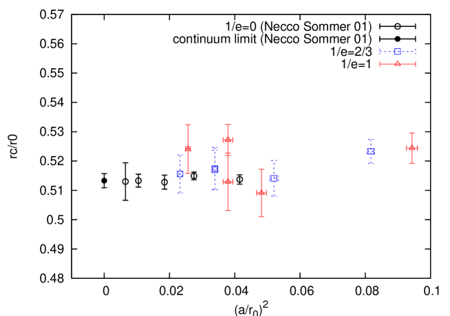
Figure 2: A ratio of the Sommer scales $r_{c}/r_{0}$. Squares and triangles are data for the topology conserving gauge action with $1/\epsilon$ = 2/3 and 1, respectively. Open circles represent the standard Wilson gauge action (from Necco:2001xg ) and the filled circle is their continuum limit.

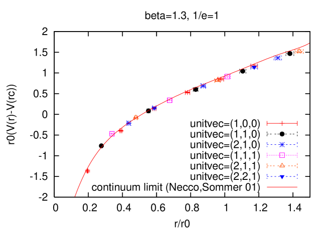
Figure 3: Static quark potential at $\beta=1.3$, $1/\epsilon$ = 1 on a $12^{4}$ lattice. The curve represents the continuum limit obtained by an interpolation of the results of Necco:2001xg . Different symbols show $V(\vec{r})$’s with different orientations parallel to $\vec{v}$’s.

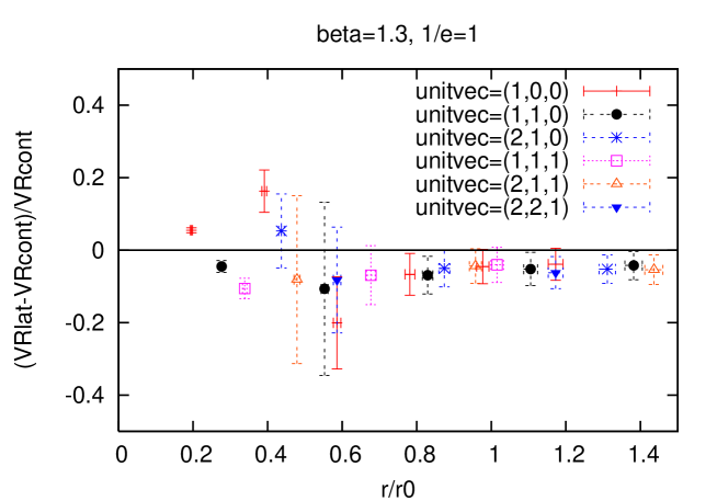
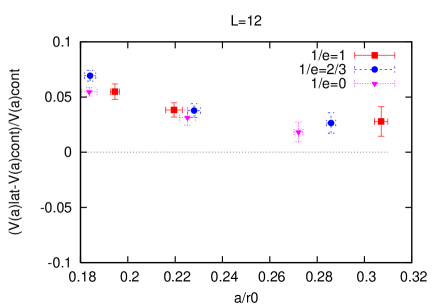
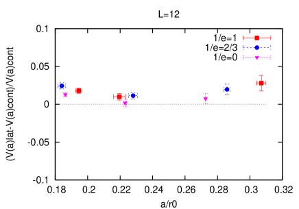
Figure 4: Violation of rotational symmetry $(\hat{V}(\vec{r})-\hat{V}_{\mathrm{cont}}(|\vec{r}|))/\hat{V}_{\mathrm{cont}}(|\vec{r}|)$, where $\hat{V}_{\mathrm{cont}}(|\vec{r}|)$ denotes the continuum limit. Results for $\beta$ = 1.3, $1/\epsilon$ = 1 are shown. The error of $\hat{V}_{\mathrm{cont}}(|\vec{r}|)$ is not taken into account ($\lesssim 1\%$).

Figure 5: $(\hat{V}(\vec{r})-\hat{V}_{\mathrm{cont}}(|\vec{r}|))/\hat{V}_{\mathrm{cont}}(|\vec{r}|)$ for $\vec{r}=(1,0,0)$. Results with different $\beta$ and $1/\epsilon$ values are plotted as a function of $a/r_{0}$. Left and right panels show the plot without and with the tree level improvement for the argument $\vec{r}$, respectively. See the text for details.

Finally, we confirm our assumption that the topology does not affect the quark potential by measuring $r_{0}$ for two initial value of $Q$ (0 and $-3$). Measurements are done on a $16^{4}$ lattice at $\beta$ = 1.42, $1/\epsilon$ = 1, for which the probability of the topology change is extremely small as discussed in the next section. Our results are $r_{0}/a$ = 6.24(9) for the $Q=0$ initial condition and 6.11(13) for $Q=-3$.

IV Perturbative renormalization of the coupling

In this section, we study whether the perturbative corrections are under control with the topology conserving gauge action.

Two-loop corrections to the gauge coupling for general actions constructed by the plaquette is available in Ellis:1983af . Using that formula, the renormalized gauge couping $g_{M}$ defined in the so-called Manton scheme is given by

$$\frac{1}{g_{M}^{2}}=\frac{1}{g^{2}}+A_{1}+A_{2}g^{2},$$ (23)

where the coefficients $A_{1}$, $A_{2}$ are calculated as

$$A_{1} = s_{4}\frac{2N_{c}^{3}-3}{N_{c}}+t_{4}(N_{c}^{2}+1),$$

$$A_{2} = a_{R}[s_{4}(2N_{c}^{2}-3)+t_{4}N_{c}(N_{c}^{2}+1)]+s_{6}\frac{15(N_{c}^{4}-3N_{c}^{2}+3)}{8N_{c}^{2}}$$ (24)

$$+u_{6}\frac{3(2N_{c}^{2}-3)(N_{c}^{2}+3)}{8N_{c}}+t_{6}\frac{3}{8}(N_{c}^{2}+1)(N_{c}^{2}+3)$$

$$-s_{4}^{2}\frac{9N_{c}^{4}-30N_{c}^{2}+36}{2N_{c}^{2}}-2s_{4}t_{4}\frac{(2N_{c}^{2}-3)(N_{c}^{2}+2)}{N_{c}}-t_{4}^{2}(N_{c}^{2}+1)(N_{c}^{2}+2).$$

Here, the parameters are $N_{c}=3$, $s_{4}=-1/4!$, $s_{6}=1/6!$, $t_{4}=1/(4N_{c}\epsilon)$, $t_{6}=1/(8N_{c}^{2}\epsilon^{2})$, $u_{6}=-1/(4!N_{c}\epsilon)$, and $a_{R}=-0.0011(2)$. Table 5 gives the next-to-leading and next-to-next-to-leading order coefficients $A_{1}$ and $A_{2}$ for various values of $\epsilon$.

Since the perturbative expansion is poorly converging if one uses the bare lattice coupling, we also consider the mean field improvement using the measured value of the plaquette expectation value Lepage:1992xa . To do so, we need a perturbative expectation value of the plaquette expectation value, which is available to the two-loop order for the general one-plaquette action Heller:1995pu as

$$\langle W(1,1)\rangle = 1-g^{2}\frac{(N_{c}^{2}-1)}{N_{c}}\bar{W}_{2}(1,1)-g^{4}(N_{c}^{2}-1)X(1,1)$$ (25)

$$+g^{4}\frac{(2N_{c}^{2}-3)(N_{c}^{2}-1)}{6N_{c}^{2}}\bar{W}_{2}(1,1)^{2}-g^{4}\frac{(N_{c}^{2}-1)}{6N_{c}}CZ(1,1).$$

Here the notations $\bar{W}_{2}(1,1)$ and $X(1,1)$ are from the original calculation Heller:1984hx for the standard Wilson gauge action, and $Z(1,1)=(1-1/V)\bar{W}_{2}(1,1)/4$ (on a symmetric lattice $V=L^{4}$) is introduced for generalization. Their values are $\bar{W}_{2}(1,1)=1/8$, $X(1,1)=-1.01\times 10^{-4}$ and $Z(1,1)=1/32$ in the infinite volume limit. The constant $C$ is written as

$$C=\left[\sum_{R}6g^{2}\frac{s_{R}(\beta)T(R)C_{2}(R)}{d_{R}}-N_{c}\right],$$ (26)

where $C_{2}(R)$ is the quadratic Casimir operator in a representation $R$ of the group $SU(N_{c})$. $d_{R}$ denotes the dimension of the representation $R$, and $T(R)$ is defined such that $\mbox{Tr}_{R}(t^{a}t^{b})=T(R)\delta^{ab}$ for the group generator $t^{a}$ in the representation $R$. The coupling $s_{R}(\beta)$ is defined when we rewrite the gauge action in terms of a general form of the one-plaquette action

$$S_{G}=\sum_{x,\mu,\nu}\sum_{R}s_{R}(\beta)\left[1-\frac{1}{d_{R}}\mbox{Re}\mbox{Tr}_{R}P^{R}_{\mu\nu}(x)\right],$$ (27)

where $P_{\mu\nu}^{R}$ denotes the plaquette in the $R$ representation. The values of these parameters for the topology conserving gauge action (4) are

$$s_{3}(\beta)=\left(1+\frac{11}{6\epsilon}\right)\beta,\;\;\;s_{6}(\beta)=-\frac{1}{3\epsilon}\beta,\;\;\;s_{8}(\beta)=-\frac{4}{9\epsilon}\beta,$$ (28)

and $T(3)=1/2$, $T(6)=5/2$, $T(8)=3$, $C_{2}(3)=4/3$, $C_{2}(6)=10/3$, $C_{2}(8)=3$. Using these numbers, we obtain $C=5-20/\epsilon$ and finally

$$\langle W(1,1)\rangle=1-\frac{g^{2}}{3}+\left(\frac{5}{18\epsilon}-\frac{5}{144}\right)g^{4}.$$ (29)

We define a boosted coupling $\bar{g}^{2}$ as

$$\frac{1}{\bar{g}^{2}}=\frac{P}{g^{2}}\left(\frac{1}{1-(1-P)/\epsilon}+\frac{(1-P)/\epsilon}{(1-(1-P)/\epsilon)^{2}}\right),$$ (30)

with the measured value of the plaquette expectation value $P=\langle W(1,1)\rangle$ (see Table 1). It is defined to be a factor in front of $F_{\mu\nu}^{2}$ when we rewrite $P_{\mu\nu}=P\exp(ia^{2}F_{\mu\nu})$ and expand the action (4). The perturbative expansion of (30) becomes

$$\frac{1}{\bar{g}^{2}}=\frac{1}{g^{2}}+B_{1}+B_{2}g^{2},$$ (31)

where

$$B_{1}=-\frac{1}{3}\left(1-\frac{2}{\epsilon}\right),\;\;\;B_{2}=\left(1-\frac{2}{\epsilon}\right)\left(\frac{5}{18\epsilon}-\frac{5}{144}\right)-\frac{2}{9\epsilon}+\frac{1}{3\epsilon^{2}}.$$ (32)

We then obtain the perturbative expansion of the Manton scheme coupling in terms of the boosted coupling

$$\frac{1}{g_{M}^{2}}=\frac{1}{\bar{g}^{2}}+(A_{1}-B_{1})+(A_{2}-B_{2})\bar{g}^{2}.$$ (33)

Numerical values of $B_{i}$ and $A_{i}-B_{i}$ are listed in Table 5. We can confirm the effect of the mean field improvement; the two-loop coefficient $A_{2}$ is significantly reduced by reorganizing the perturbative expansion as in (33).

$1/\epsilon$	$A_{1}$	$A_{2}$	$B_{1}$	$B_{2}$	$A_{1}-B_{1}$	$A_{2}-B_{2}$
0	$-$0.20833	$-$0.03056	$-$0.33333	$-$0.03472	0.12500	0.00416
2/3	0.34722	$-$0.04783	0.11111	$-$0.05015	0.23611	0.00233
1	0.62500	$-$0.10276	0.33333	$-$0.13194	0.29167	0.02919

Table 5: Next-to-leading and next-to-next-to-leading order coefficients for the coupling renormalization for various $\epsilon$. Mean field improved coefficients $A_{1}-B_{1}$, $A_{2}-B_{2}$ are also shown. See the text for details.

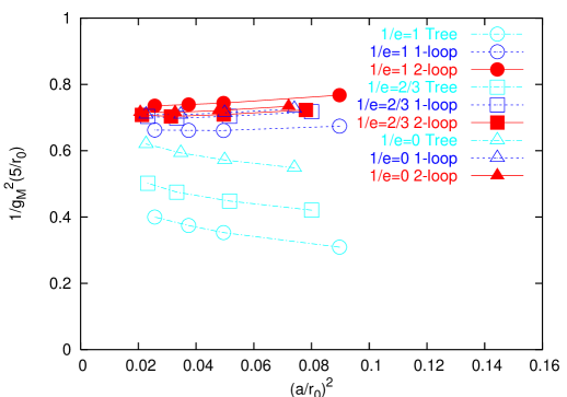
Figure 6: $1/g_{M}^{2}$ in the Manton scheme for various values of $1/\epsilon$. The mean field improved expression (33) is used with the measured plaquette expectation value. Different symbols distinguish the value of $1/\epsilon$ (1 for circles, 2/3 for squares, 0 for triangles). Open symbols with dot-dashed line represent tree-level results and open symbols with dashed lines are one-loop. The best results including two-loop corrections are shown by filled symbols with solid lines.

Using these results, the inverse squared renormalized coupling in the Manton scheme is obtained for each lattice parameters. In Figure 6 we plot the coupling evaluated at a reference scale $5/r_{0}$ as a function of lattice scaling squared. We use the two-loop renormalization equation for the evolution to the reference scale. Although the couplings are very different at the tree level, the one-loop results are already in good agreement among the different values of $1/\epsilon$. Including the two-loop corrections, we find that the perturbative expansion converges very well and the agreement among different $1/\epsilon$ becomes even better. Good scaling toward the continuum limit can also be observed in this plot for the two-loop results.

V Stability of the topological charge

In this section we discuss the stability of the topological charge with the topology conserving gauge action.

How the topological charge is preserved can be easily explained in the U(1) gauge theory in two-dimension, for which we can define an exact geometrical definition of the topological charge Luscher:1998kn ; Luscher:1998du

$$Q_{\mathrm{geo}} = \frac{1}{2\pi}\sum_{x}\frac{1}{2}\epsilon_{\mu\nu}F^{\mathrm{lat}}_{\mu\nu}(x),$$

$$F^{\mathrm{lat}}_{\mu\nu}(x) = -i\ln(P_{\mu\nu}(x)),\;\;\;-\pi<F^{\mathrm{lat}}_{\mu\nu}(x)\leq\pi.$$ (34)

$P_{\mu\nu}(x)$ denotes the plaquette in the U(1) gauge theory. In two dimensions, $Q_{\mathrm{geo}}$ gives an integer on the lattices with the periodic boundary condition. The topological charge may change its value when the field strength pass through the point $F^{\mathrm{lat}}_{\mu\nu}(x)=\pm\pi$. Since the jump from $F^{\mathrm{lat}}_{\mu\nu}(x)=-\pi$ to $F^{\mathrm{lat}}_{\mu\nu}(x)=+\pi$ is allowed with the usual compact and non-compact gauge actions, the topology change may occur without a big penalty. It is the U(1) version of the Lüscher’s bound

$$1-\mbox{Re}P_{\mu\nu}(x)<\epsilon$$ (35)

with $\epsilon<2$, that can prevent these topology changes because the point $F^{\mathrm{lat}}_{\mu\nu}(x)=\pm\pi$ is not allowed under this condition. Furthermore, it can be shown that $Q_{\mathrm{geo}}$ is equivalent to the index of the overlap fermion with $s=0$ if $\epsilon<1/5$ is satisfied.

For the non-abelian gauge theories in higher dimensions, we do not have the exact geometrical definition of the topological charge (note that (6) gives non-integers). It is, however, quite natural to assume that a similar mechanism concerning the compactness of the link variables allows us to preserve the index of the overlap-Dirac operator for very small $\epsilon$. Also for larger $\epsilon$, we may expect that the topology stabilizes well in practical sampling of gauge configurations.

Table. 6 summarized our data for the stability of the topological charge

$$\mbox{Stab}_{Q}\equiv\frac{N_{\mathrm{trj}}}{\tau_{\mathrm{plaq}}\times\#Q},$$ (36)

where $\tau_{\mbox{\tiny plaq}}$ is the autocorrelation time of the plaquette, measured using the method described in Appendix E of Luscher:2004rx . $N_{\mbox{\tiny trj}}$ denotes the total length of the HMC trajectories and $\#Q$ is the number of topology changes during the trajectories. The topological charge $Q$ is measured every 10–20 trajectories with the geometrical definition (6) after our cooling method. With this definition, $\mbox{Stab}_{Q}$ represents a mean number of independent gauge configurations sampled staying a certain topological charge. But it only gives an upper limit, because the topology change is detected only every 10–20 trajectories and we may miss the change if $Q$ changes its value and returns to the original value between two consecutive measurements. Therefore, our measurement of $\mbox{Stab}_{Q}$ may give a good approximation when the topology change is a rare event.

Lattice size	$1/\epsilon$	$\beta$	$r_{0}/a$	$N_{\mbox{\tiny trj}}$	$\tau_{\mbox{\tiny plaq}}$	$\#Q$	StabQ
$12^{4}$	1	1.0	3.257(30)	18000	2.91(33)	696	9
		1.2	4.555(73)	18000	1.59(15)	265	43
		1.3	5.140(50)	18000	1.091(70)	69	239
	2/3	2.25	3.498(24)	18000	5.35(79)	673	5
		2.4	4.386(53)	18000	2.62(23)	400	17
		2.55	5.433(72)	18000	2.86(33)	123	51
	0	5.8	[3.668(12)]	18205	30.2(6.6)	728	1
		5.9	[4.483(17)]	27116	13.2(1.5)	761	3
		6.0	[5.368(22)]	27188	15.7(3.0)	304	6
$16^{4}$	1	1.3	5.240(96)	11600	3.2(6)	78	46
		1.42	6.240(89)	5000	2.6(4)	2	961
	2/3	2.55	5.290(69)	12000	6.4(5)	107	18
		2.7	6.559(76)	14000	3.1(3)	6	752
	0	6.0	[5.368(22)]	3500	11.7(3.9)	14	21
		6.13	[6.642(–)]	5500	12.4(3.3)	22	20
$20^{4}$	1	1.3	—	1240	2.6(5)	14	34
		1.42	—	7000	3.8(8)	29	64
	2/3	2.55	—	1240	3.4(7)	15	24
		2.7	—	7800	3.5(6)	20	111
	0	6.0	—	1600	14.4(7.8)	37	3
		6.13	—	1298	9.3(2.8)	4	35

Table 6: Stability of the topological charge $\mbox{Stab}_{Q}$. The length of the HMC trajectory $N_{\mbox{\tiny trj}}$, the autocorrelation time measured for plaquette $\tau_{\mbox{\tiny plaq}}$, and the number of topology change $\#Q$ are also summarized.

Results are plotted in Figure 7 as a function of the lattice spacing squared. We find a clear trend that the stability increases for larger $1/\epsilon$ if the lattice spacing is the same. When the lattice size is increased from $L/a$ = 12 to 16, the stability drops significantly for each value of $1/\epsilon$. This is expected, because the topology change occurs through local dislocations of gauge field and its probability scales as the volume. For even larger volume ($L/a$ = 20), our data are not precise enough, since the total length of trajectory is shorter. We also observe that the stability increases very rapidly toward the continuum limit.

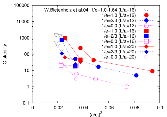
Figure 7: Stability of the topological charge. Different symbols represent the lattice size: $L/a$ = 12 (circles), 16 (squares), 20 (upward triangles). The value of $1/\epsilon$ is distinguished by the line type: $1/\epsilon$ = 0 (dotted), 2/3 (dashed), 1 (solid). Downward triangles are the data of Bietenholz:2004mq measured on 16⁴ lattices.

For the study of the $\epsilon$-regime in a fixed topological sector, the lattices $(1/\epsilon,\beta,L)\sim(1,1.42,16)$ and $(2/3,2.7,16)$ would be appropriate. Their physical size is $L\sim$ 1.25 fm and the topological charge is stable for $(100-1000)\tau_{\mathrm{plaq}}$ trajectories.

VI Construction of the overlap-Dirac operator

VI.1 Low-lying mode distribution of $H_{W}$

We measure the low-lying eigenvalues of $aH_{W}$ on the gauge configurations generated with the topology conserving gauge action. We use the numerical package ARPACK ARPACK , which implements the implicitly restarted Arnoldi method. For the hermitian Wilson-Dirac operator $aH_{W}$ we take the form $aH_{W}=\gamma_{5}(aD_{W}-1-s)$ with $s=0.6$.

Figure 8 shows a typical comparison of the eigenvalue distribution for three values of $1/\epsilon$ on a 20⁴ lattice. The $\beta$ value is chosen such that the Sommer scale $r_{0}/a$ is roughly equal to 5.3, which corresponds to $a\simeq 0.1$ fm. From the plot we observe that the density of the low-lying modes is relatively small for larger values of $1/\epsilon$. To quantify this statement we list the probability, $P(<0.1)$, to find the eigenvalue smaller than 0.1 in Table 7. For the above example, the probability is 41% for the standard Wilson gauge action ($1/\epsilon$ = 0), but it decreases to 15% (9%) for $1/\epsilon$ = 2/3 (1). For another lattice spacing ($r_{0}/a\simeq$ 6.5) and lattice size $16^{4}$, a similar trend can be found. In Table 7 we also summarize the ensemble average of the lowest eigenvalue $\lambda_{\mathrm{min}}$ and the inverse of condition numbers $\lambda_{\mathrm{max}}/\lambda_{\mathrm{min}}$ and $\lambda_{\mathrm{max}}/\lambda_{\mathrm{10}}$, where $\lambda_{\mathrm{10}}$ and $\lambda_{\mathrm{max}}$ denote the 10th and the highest eigenvalues respectively. We may conclude that the lowest eigenvalue is higher in average for larger $1/\epsilon$.

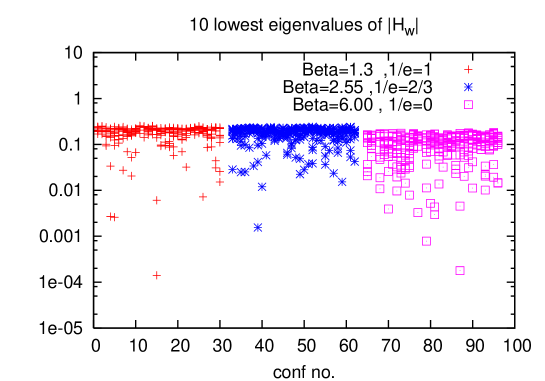
Figure 8: Ten lowest eigenvalues of $|aH_{W}|=|\gamma_{5}(aD_{W}-1.6)|$ for gauge configurations with $r_{0}/a\simeq 5.3$. Data are shown for $1/\epsilon$ = 1 (pluses), 2/3 (stars), and 0 (squares). The lattice size is 20⁴.

lattice size	$1/\epsilon$	$\beta$	$r_{0}/a$	$P(<0.1)$	$\lambda_{\mathrm{min}}$	$\lambda_{\mathrm{min}}/\lambda_{\mathrm{max}}$	$\lambda_{\mathrm{10}}/\lambda_{\mathrm{max}}$
$20^{4}$	1	1.3	5.240(96)	0.090(14)	0.0882(84)	0.0148(14)	0.03970(29)
	2/3	2.55	5.290(69)	0.145(12)	0.0604(53)	0.0101(08)	0.03651(27)
	0	6.0	[5.368(22)]	0.414(29)	0.0315(57)	0.0059(34)	0.02766(46)
	1	1.42	6.240(89)	0.031(10)	0.168(13)	0.0282(21)	0.04765(32)
	2/3	2.7	6.559(76)	0.019(18)	0.151(11)	0.0251(19)	0.04646(37)
	0	6.13	[6.642(–)]	0.084(14)	0.0861(83)	0.0126(15)	0.03775(50)
$16^{4}$	1	1.3	5.240(96)	0.053(13)	0.111(12)	0.0187(21)	0.04455(31)
	2/3	2.55	5.290(69)	0.067(13)	0.1038(98)	0.0174(16)	0.04239(36)
	0	6.0	[5.368(22)]	0.130(20)	0.0692(90)	0.0116(15)	0.03451(62)
	1	1.42	6.240(89)	0.007(5)	0.219(13)	0.0367(21)	0.05233(26)
	2/3	2.7	6.559(76)	0.020(8)	0.191(12)	0.0320(19)	0.05117(29)
	0	6.13	[6.642(–)]	0.030(10)	0.139(10)	0.0232(17)	0.04384(38)

Table 7: The probability $P(<0.1)$ to find the eigenvalue lower than 0.1 for the hermitian Wilson-Dirac operator $|aH_{W}|=|\gamma_{5}(aD_{W}-1.6)|$. Ensemble averages of the lowest eigenvalue and the inverse of condition numbers are also listed. The Sommer scale $r_{0}/a$ is the results for $L=16$ lattices. The values with [] are from Necco:2001xg with an interpolation in $\beta$.

VI.2 Numerical cost

In the numerical implementation of the overlap-Dirac operator one often subtracts the low-lying eigenmodes of $aH_{W}$ and treats them exactly. The rest of the modes are approximated by some polynomial or rational functions. The numerical cost to operate the overlap-Dirac operator is dominated by the polynomial/rational part, because the subtraction have to be done only once for a given configuration. Here, we assume that 10 lowest eigenmodes are subtracted and compare the relative numerical cost on the gauge configurations with different values of $1/\epsilon$.

The accuracy of the Chebyshev polynomial approximation $\mbox{sgn}_{\mathrm{Cheb}}(aH_{W})$ with a degree $N_{\mathrm{poly}}$ can be expressed as Giusti:2002sm

$$\frac{\langle v|(1-\mbox{sgn}_{\mathrm{Cheb}}^{2}(aH_{W}))^{2}|v\rangle}{\langle v|v\rangle}\sim A\exp(-BN_{\mathrm{poly}}/\kappa),$$ (37)

for a random noise vector $|v\rangle$. $A$ and $B$ are constants. We find that they are $A\sim$ 0.3 and $B\sim$ 4.2 almost independent of the lattice parameters as shown in Figure 9. The reduced condition number $\kappa=\lambda_{\mathrm{max}}/\lambda_{\mathrm{10}}$ enters in the formula with a combination $N_{\mathrm{poly}}/\kappa$. Therefore, the numerical cost, which is proportional to $N_{\mathrm{poly}}$, depends linearly on $\kappa$ if one wants to keep the accuracy for the sign function. From Table 7 we observe that the reduced condition number is about a factor 1.2–1.4 smaller for $1/\epsilon$ = 1 than that for the standard Wilson gauge action.

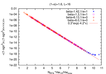
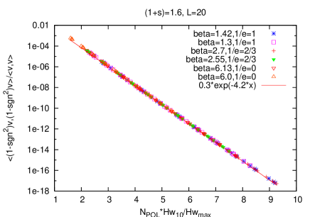
Figure 9: The accuracy (37) as a function of $N_{\mathrm{pol}}/\kappa$ for $L$ = 16 (left) and $L$ = 20 (right). We use 4 gauge configurations and 10 values of $N_{\mathrm{pol}}$ = 60–195 for each parameter set.

We also check that the above observation does not change by varying the value of $s$ in a reasonable range. Figure 10 shows a typical distribution of the low-lying eigenmodes for $s$ = 0.2–0.7. We find that the advantage of the topology conserving gauge action does not change. Also, from these plots we can see that $s\sim 0.6$ is nearly optimal for all cases.

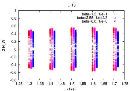
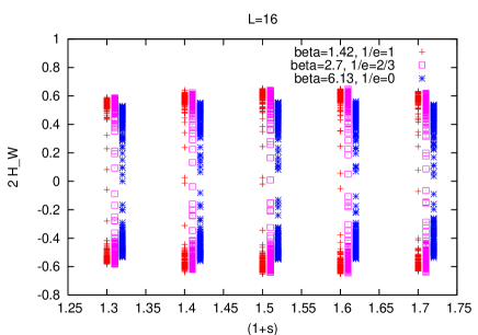
Figure 10: Ten near-zero eigenvalues for $r_{0}/a\sim 5.3$ (left) and $r_{0}/a\sim 6.5$ (right). Results are plotted as a function of $1+s$. Data for $1/\epsilon$ = 2/3 and 0 are slightly shifted for clarity.

VI.3 Locality

If the overlap-Dirac operator is local, the norm $||D(x,y)v(y)||$ with a point source vector $v$ at $x_{0}$ should decay exponentially as a function of $x-x_{0}$ Hernandez:1998et

$$||D(x,y)v(y)||\sim C\exp(-D|x-x_{0}|)$$ (38)

with constants $C$ and $D$. This behavior is actually observed in Figure 11. The plots are shown for different values of $1/\epsilon$ at the lattice scales $r_{0}/a\simeq$ 5.3 (left) and 6.5 (right). We find no remarkable difference on the locality for different gauge actions.

Recently, it has been pointed out that the mobility edge is the crucial quantity which governs the locality of the overlap-Dirac operator Golterman:2003qe ; Golterman:2004cy ; Golterman:2005fe ; Svetitsky:2005qa . It would be interesting to see the dependence of the mobility edge on the parameters in the topology conserving action, which is left for future works.

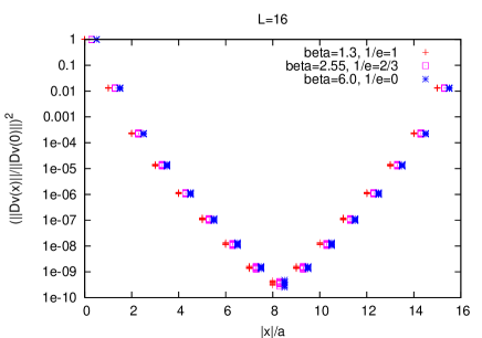
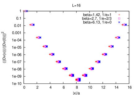
Figure 11: $(||D(x,y)v(y)||/||D(0,y)v(y)||)^{2}$ with $x_{0}=0$ measured on 10 gauge configurations for different values of $1/\epsilon$. The lattice scale is $r_{0}/a\simeq 5.3$ (left) and 6.5 (right).

VII Conclusions

We study the properties of the topology conserving gauge action (4) in the quenched approximation. For small $\epsilon$ ($\lesssim$ 1/20), the parameter to control the admissibility of the plaquette variable, it is theoretically known that the topology change is strictly prohibited, but we investigate the action with $\epsilon\sim O(1)$ for the use of practical purposes. With the (quenched) Hybrid Monte Carlo updation, we find that the topology change is strongly suppressed for $1/\epsilon$ = 2/3 and 1, compared to the standard Wilson gauge action. The topological charge becomes more stable for fine lattices, and it is possible to preserve the topological charge for O(1,000) HMC trajectories at $a\simeq$ 0.08 fm and $L\simeq$ 1.3 fm. In the same parameter region, the standard Wilson gauge action changes the topological charge every $O(10)$ trajectories. The action is therefore proved to be useful to accumulate gauge configurations in a fixed topological sector.

We measure the heavy quark potential with this gauge action at $1/\epsilon$ = 2/3 and 1. The lattice spacing is determined from the Sommer scale $r_{0}$. With these measurements we also investigate the scaling violation for short and intermediate distances. The probe in the short distance is the violation of the rotational symmetry, and a ratio $r_{c}/r_{0}$ of two different scale can be used for the intermediate distances. For both of these we find that the size of the scaling violation is comparable to the standard Wilson gauge action, which is consistent with the expectation that the term with $1/\epsilon$ introduces a difference at most $O(a^{4})$. The action (4) shows no disadvantage as far as the scaling is concerned.

The perturbative expansion of the coupling and Wilson-loops is available in the literature for general one-plaquette action. We write down the coefficients for our particular action (4) and observe that the convergence is very good if the mean field improvement is applied. The coupling constant in a certain scheme at a given scale is consistent among different values of $1/\epsilon$.

As a result of the (approximate) topology conservation, the low-lying eigenvalues of the Wilson-Dirac operator in the negative mass regime is suppressed. This is an advantage in the construction of the overlap-Dirac operator, since the numerical cost to evaluate the sign function is proportional to the inverse of the lowest eigenvalue for a given gauge configuration. In this case, the gain is about a factor 2–3 at the same lattice spacing compared to the standard Wilson gauge action. If the first several eigenmodes are subtracted and treated exactly, the gain is marginal, 20–40%. Similar improvements have been observed with the improved gauge actions, such as the Lüscher-Weisz, Iwasaki and DBW2.

References

- (1) H. Neuberger, Phys. Lett. B 417, 141 (1998) [arXiv:hep-lat/9707022].
- (2) H. Neuberger, Phys. Lett. B 427, 353 (1998) [arXiv:hep-lat/9801031].
- (3) M. Lüscher, Phys. Lett. B 428, 342 (1998) [arXiv:hep-lat/9802011].
- (4) P. H. Ginsparg and K. G. Wilson, Phys. Rev. D 25, 2649 (1982).
- (5) P. Hernandez, K. Jansen and M. Lüscher, Nucl. Phys. B 552, 363 (1999) [arXiv:hep-lat/9808010].
- (6) H. Neuberger, Phys. Rev. D 61, 085015 (2000) [arXiv:hep-lat/9911004].
- (7) M. Lüscher, Nucl. Phys. B 549, 295 (1999) [arXiv:hep-lat/9811032].
- (8) H. Fukaya and T. Onogi, Phys. Rev. D 68, 074503 (2003) [arXiv:hep-lat/0305004].
- (9) H. Fukaya and T. Onogi, D 70, 054508 (2004) [arXiv:hep-lat/0403024].
- (10) S. Shcheredin, W. Bietenholz, K. Jansen, K. I. Nagai, S. Necco and L. Scorzato, arXiv:hep-lat/0409073.
- (11) W. Bietenholz, K. Jansen, K. I. Nagai, S. Necco, L. Scorzato and S. Shcheredin [XLF Collaboration], AIP Conf. Proc. 756, 248 (2005) [arXiv:hep-lat/0412017].
- (12) S. Shcheredin, arXiv:hep-lat/0502001.
- (13) K. i. Nagai, K. Jansen, W. Bietenholz, L. Scorzato, S. Necco and S. Shcheredin, Proc. Sci. LAT2005, 283 (2005) [arXiv:hep-lat/0509170].
- (14) M. Lüscher and P. Weisz, Phys. Lett. B 158, 250 (1985).
- (15) Y. Iwasaki, Nucl. Phys. B 258, 141 (1985); Univ. of Tsukuba Report UTHEP-118 (1983) unpublished.
- (16) P. de Forcrand et al. [QCD-TARO Collaboration], Nucl. Phys. B 577, 263 (2000) [arXiv:hep-lat/9911033].
- (17) T. DeGrand, A. Hasenfratz and T. G. Kovacs, Phys. Rev. D 67, 054501 (2003) [arXiv:hep-lat/0211006].
- (18) Z. Fodor, S. D. Katz and K. K. Szabo, JHEP 0408, 003 (2004) [arXiv:hep-lat/0311010].
- (19) C. Morningstar and M. J. Peardon, Phys. Rev. D 69, 054501 (2004) [arXiv:hep-lat/0311018].
- (20) M. Creutz, Phys. Rev. D 70, 091501(R) (2004) [arXiv:hep-lat/0409017].
- (21) S. Duane, A. D. Kennedy, B. J. Pendleton and D. Roweth, Phys. Lett. B 195, 216 (1987).
- (22) J. Hoek, M. Teper and J. Waterhouse, Nucl. Phys. B 288, 589 (1987).
- (23) M. Lüscher, Nucl. Phys. B 538, 515 (1999) [arXiv:hep-lat/9808021].
- (24) A. Gonzalez-Arroyo, arXiv:hep-th/9807108.
- (25) L. Giusti, C. Hoelbling, M. Lüscher and H. Wittig, Comput. Phys. Commun. 153, 31 (2003) [arXiv:hep-lat/0212012].
- (26) G. S. Bali and K. Schilling, Phys. Rev. D 46, 2636 (1992).
- (27) M. Guagnelli, R. Sommer and H. Wittig [ALPHA collaboration], Nucl. Phys. B 535, 389 (1998) [arXiv:hep-lat/9806005].
- (28) S. Necco and R. Sommer, Nucl. Phys. B 622, 328 (2002) [arXiv:hep-lat/0108008].
- (29) M. Lüscher, arXiv:hep-lat/0409106.
- (30) R. K. Ellis and G. Martinelli, Nucl. Phys. B 235, 93 (1984) [Erratum-ibid. B 249, 750 (1985)].
- (31) G. P. Lepage and P. B. Mackenzie, Phys. Rev. D 48, 2250 (1993) [arXiv:hep-lat/9209022].
- (32) U. M. Heller, Nucl. Phys. B 451, 469 (1995) [arXiv:hep-lat/9502009].
- (33) U. M. Heller and F. Karsch, Nucl. Phys. B 251, 254 (1985).
- (34) ARPACK, available from http://www.caam.rice.edu/software/ARPACK/
- (35) M. Golterman and Y. Shamir, Phys. Rev. D 68, 074501 (2003) [arXiv:hep-lat/0306002].
- (36) M. Golterman, Y. Shamir and B. Svetitsky, Phys. Rev. D 71, 071502(R)(2005) [arXiv:hep-lat/0407021].
- (37) M. Golterman, Y. Shamir and B. Svetitsky, Phys. Rev. D 72, 034501 (2005) [arXiv:hep-lat/0503037].
- (38) B. Svetitsky, Y. Shamir and M. Golterman, arXiv:hep-lat/0508015.