DFTT 27/05

IFUP-TH 2005-30

DIAS-STP-05-11

On the effective string spectrum of the tridimensional $\mathbb{Z}_{2}$ gauge model

M. Caselle^a, M. Hasenbusch^b and M. Panero^c

^a Dipartimento di Fisica Teorica dell’Università di Torino and I.N.F.N.,

Via Pietro Giuria 1, I-10125 Torino, Italy

e–mail:          caselle@to.infn.it

^b Dipartimento di Fisica dell’Università di Pisa and I.N.F.N.,

Largo Bruno Pontecorvo 3, I-56127 Pisa, Italy

e–mail:          Martin.Hasenbusch@df.unipi.it

^c School of Theoretical Physics, Dublin Institute for Advanced Studies,

10 Burlington Road, Dublin 4, Ireland

e–mail:          panero@stp.dias.ie

We study the $\mathbb{Z}_{2}$ lattice gauge theory in three dimensions, and present high precision estimates for the first few energy levels of the string spectrum. These results are obtained from new numerical data for the two-point Polyakov loop correlation function, which is measured in the 3d Ising spin system using duality. This allows us to perform a stringent comparison with the predictions of effective string models. We find a remarkable agreement between the numerical estimates and the Nambu-Goto predictions for the energy gaps at intermediate and large distances. The precision of our data allows to distinguish clearly between the predictions of the full Nambu-Goto action and the simple free string model up to an interquark distance $r\approx 10/\sqrt{\sigma}$. At the same time, our results also confirm the breakdown of the effective picture at short distances, supporting the hypothesis that terms which are not taken into account in the usual Nambu-Goto string formulation yield a non-trivial shift to the energy levels. Furthermore, we discuss the theoretical implications of these results.

1 Introduction

Understanding in detail the mechanisms which govern the behaviour of physical observables in the confinement phase of quantum gauge theories is still a challenge. Even the simplest confined system — a heavy quark-antiquark pair in a pure gauge model without dynamical matter fields — is a setting where a number of interesting aspects become manifest; the potential associated with such a system is asymptotically linearly rising at large interquark distances, whereas at finite distance it develops non-trivial corrections, which are expected to be predicted by some kind of effective theory.

The idea that the confining flux lines joining the two colour sources get squeezed in a thin tube explains that at asymptotically large distances the potential energy of the system is proportional to the quark-antiquark distance $r$. Assuming that the tube vibrates along the transverse directions, one can derive effective string corrections affecting the potential $V(r)$ for finite values of $r$. This infrared picture breaks down as $r$ approaches $1/m$ from above, where $m$ is the mass of the lightest glueball. At these small distances, glueball radiation has to be taken into account, leading to effects that cannot be described by the effective string model and which are specific to the given gauge model.

The theoretical background of the effective string in this setting is well-known: the pioneering works by Lüscher, Münster, Symanzik and Weisz [1, 2, 3] date back to the Eighties, and over the last decades considerable progress has been achieved in understanding the details of the picture [4, 5, 6, 7, 8, 9, 10, 11, 12].

These theoretical predictions can be confronted with data obtained from lattice gauge theory: One can check the extent to which the theoretical expectations actually match the results of Monte Carlo simulations for a wide range of parameters and for different types of gauge theories, in particular simpler prototype models for confinement than QCD [13, 14, 15, 16, 17, 18, 19, 20, 21, 22, 23].

The aim of this work is to study numerically the fine details in the behaviour of the excitation energies $E_{n}(r)$ which contribute to the partition function $Z(r,L)$ describing the confined quark-antiquark ($Q\bar{Q}$) system in Euclidean space-time with a compactified direction of size $L$:

$$Z_{Q\bar{Q}}(r,L)=\sum_{n=0}^{\infty}w_{n}e^{-E_{n}(r)L}$$ (1)

where $w_{n}$ is the multiplicity factor associated with the energy level $E_{n}$. Neglecting glueball radiation, such a partition function is proportional to the two-point correlation function among Polyakov lines $G(r)$, which can be evaluated in numerical simulations.

Here, we focus our attention onto the results obtained from the confining phase of $\mathbb{Z}_{2}$ lattice gauge theory in three dimensions: a model whose properties (remarkably, its duality with respect to the Ising spin model) are well-known, and allow to reach high precision in the determination of the interquark potential, even for large values of the interquark distance $r$, or of the lattice size in the time-like direction $L$. This in turn allows very stringent comparisons with the existing theoretical descriptions and in particular with the effective string models which we shall discuss below. In particular in this paper we will concentrate on the study of the behaviour of the first few energy levels $E_{n}$ as a function of the interquark distance $r$. We will compare our numerical data with the predictions of both the Nambu-Goto (NG) model and its free string limit. Although these two models give very similar results, the precision of our numerical simulation is sufficient to distinguish between them. We shall see that while the lowest state $E_{0}$ shows deviations from the effective string prediction even for rather large distances (as already pointed out in several papers) the energy gap $E_{1}-E_{0}$ clearly approaches the prediction of the Nambu-Goto effective string model as the distance increases. This suggests that the breakdown of the effective string model is due to additional contributions at short distances which lead to an overall shift on the effective string spectrum. In addition to gauge model specific effects, such as glueball radiation, such a contribution might be due to the so-called Liouville mode, which is neglected in deriving the effective string model predictions from the original reparametrisation-invariant string action.

Let us finally mention that other studies of the excited states of the spectrum for a static quark-antiquark pair have been done in recent years, both in the Ising model and in other LGT’s [18, 19, 20, 21, 22, 23], but they used different numerical techniques and did not reach distances large enough to appreciate the effects that we discuss in this paper. The novelty of our approach is that, by suitably combining the results of our simulations for all intermediate values or the interquark distance, we were able to directly evaluate the partition function of the model eq. (1). From it, by fitting its functional dependence on the energy levels — see the right-hand side of eq. (1) — for different values of $r$ and $L$ we could extract high precision estimates of the first few energy levels.

This paper is organised as follows. In section 2 we will recall some basic theoretical ideas underlying the effective description of the interquark potential, focusing our attention onto the bosonic string models that are expected to mimic its large distance behaviour; in particular, we will discuss the Nambu-Goto string and its free string limit. In section 3, after reviewing the basic properties of the $\mathbb{Z}_{2}$ lattice gauge theory in $D=3$, we will present the features of our simulation algorithm. Then, in section 4 we will show the numerical results; the latter will be discussed in section 5, in a comparison with similar studies; finally, we will conclude with a few remarks.

2 Theory

A quantitative description of the $Q\bar{Q}$ potential in confining gauge theories — see [24] and references therein for a review — can be formulated in terms of effective models, which are expected to provide phenomenologically consistent predictions for the behaviour of $V(r)$ in the regime of interquark distances typical of the hadronic world.

At large enough interquark distances, the region of the perturbative vacuum among two heavy sources gets “stretched” into a vortex-like configuration, whose excitations correspond to string-like modes: this is the scenario underlying the renowned effective string picture for confinement in the IR [1, 2, 3], based on the idea that the flux lines among the sources in a pure gauge theory get squeezed in a thin, almost uni-dimensional tube. As a consequence, the asymptotic behaviour of the potential is a linear rise. Remarkably enough, according to this picture, in principle one can obtain physical information about the confined system without knowing the dynamics of the microscopic degrees of freedom and the details of the gauge group.

In the following of this paper, we focus on sufficiently large interquark distances, where the effective string picture holds, and try to identify the string model which yields predictions that match best with our numerical results for the energy spectrum.

At finite distances, the leading correction to the linear interquark potential predicted by the effective string model is a Casimir effect due to the (harmonic) oscillations that can set in the finite-size string with fixed ends: they induce a $1/r$ contribution to the IR interquark potential:

$$V(r)=\sigma r+\mu-\frac{\pi(D-2)}{24r}+O\left(\frac{1}{r^{2}}\right)$$ (2)

where $D$ is the number of space-time dimensions, $\sigma$ is the string tension, and $\mu$ is a constant. The $1/r$ term in eq. (2) is known as the “Lüscher term”: it can be predicted under the assumption that, at leading order, the string fluctuations along the $D-2$ transverse directions are described by free, massless boson fields, and its numerical coefficient can also be obtained via CFT arguments.

According to this “free string” picture, the excitation spectrum is expected to be simply described as a tower of equally-spaced levels labelled by a non-negative integer $n$:

$$E_{n}=E_{0}+\frac{\pi}{r}n$$ (3)

and, in general, degeneracies are expected for $n\geq 1$.

The prediction for $V(r)$ in eq. (2) can be refined, making more precise assumptions about the dynamics describing string vibrations: more precisely, the partition function $Z(r,L)$ associated to the $Q\bar{Q}$ sector of the gauge theory (which approximates the Polyakov loop two-point correlation function $G(r)$) can be expressed as a string partition function:

$$G(r)=\langle P^{\dagger}(r)P(0)\rangle=\int\left[\mathcal{D}h\right]e^{-S_{\mbox{\tiny{eff}}}}$$ (4)

where $S_{\mbox{\tiny{eff}}}$ denotes the effective action for the world sheet spanned by the string. In eq. (4), the functional integration is done over world sheet configurations which have fixed boundary conditions along the space-like direction, and periodic boundary conditions along the compactified, time-like direction — the Polyakov lines being the fixed boundary of the string world sheet. In general, the effective string action $S_{\mbox{\tiny{eff}}}$ describing string dynamics also encodes string interactions.

A particular choice for $S_{\mbox{\tiny{eff}}}$ is to assume that it is proportional to the area spanned by the string world sheet:

$$S_{\mbox{\tiny{eff}}}=\sigma\cdot\int d^{2}\xi\sqrt{\det g_{\alpha\beta}}$$ (5)

which is the Nambu-Goto action [25, 26, 27].

The Nambu-Goto model can be quantised along two almost equivalent ways:

a] Fix the reparametrisation and Weyl invariance of eq. (5) using the so-called physical gauge (see for instance [4, 7]) in which the longitudinal degrees of freedom of the string are identified with the coordinates of the plane in which the two Polyakov loops lie. This gauge choice is anomalous (unless $D=26$) [28]: the anomaly manifests itself as a breaking of Lorentz invariance, but it can be shown that the anomalous contribution is a rapidly decreasing function of the interquark distance [9]. The effective string model is the quantum field theory which one obtains by simply neglecting this anomaly. The obvious implication of this assumption is that the effective string theory predictions are bound to hold only for large enough interquark distances. The critical distance below which the picture is no longer valid cannot be deduced from the theory. It can only be obtained numerically by comparing prediction and simulations. In the limit in which the anomaly can be neglected it is possible to proceed to formal quantisation of the resulting action [4, 7] — which has now been reduced to an ordinary QFT of the transverse degrees of freedom only, interacting via a square-root-type potential. The spectrum obtained in this way is:

$$E_{n}(r)=\sigma r\sqrt{1+\frac{2\pi}{\sigma r^{2}}\left(n-\frac{D-2}{24}\right)}\;\;,\;\;\;\;n\in\mathbb{N}$$ (6)

and the $w_{n}$’s — i.e. the multiplicity factors which appear in eq. (1) — are given by:

$$w_{n}=\sum^{n}_{i_{1}=0}\dots\sum^{n}_{i_{D-2}=0}\left[P\left(i_{1}\right)\dots P\left(i_{D-2}\right)\delta_{n,i_{1}+\dots+i_{D-2}}\right]$$ (7)

where $P(i)$ denotes the number of partitions of $i$. In particular, in three space-time dimensions, the $w_{n}$ coefficients are simply the partitions of $n$, and we end up with the following expression for the effective string partition function:

$$Z_{Q\bar{Q}}(r,L)=\sum_{n=0}^{\infty}P(n)e^{-E_{n}(r)L}$$ (8)

b] Alternatively, one could use the reparametrisation invariance to reach the conformal gauge (where the NG action is equivalent to the free string action) and then quantize it using the so-called covariant quantisation [29, 30] in the background of two “zero branes”, which play the role of the Polyakov loops. In this framework, the anomaly shows up with the appearance of an additional field (the so-called “Liouville mode”). If one assumes, as above, that at large distance this mode can be neglected, then one can quantize the string as it is usually done for the critical bosonic string, and re-obtain all the previous results [31]. In particular, one exactly finds the Nambu-Goto spectrum of eq. (6). The major advantage of the latter procedure is that it makes the role of the Liouville mode explicit, and it could in principle offer a clue to guess its contribution to the effective string prediction at shorter interquark distances.

One should stress that the Nambu-Goto action is by no reason the only possible choice for the effective string action. It is the simplest choice and has a nice geometrical interpretation. Thus in these last years much effort has been devoted to the construction of alternative string actions. Among these a particularly interesting proposal appeared a few years ago in [11]. We shall not further discuss this proposal in the present paper, we only mention here that it can be shown that the first two perturbative orders in the string tension expansion of this effective string coincide with the Nambu-Goto ones [32] and thus, at least at low temperature and large distance, the two effective strings should follow the same behaviour.

3 General setting and the algorithm

In this paper, we restrict our attention to the $\mathbb{Z}_{2}$ lattice gauge theory in $D=3$: the dynamics of the $U_{\mu}(x)$ bond variables (taking values in $\mathbb{Z}_{2}$) is expressed by the standard Wilson action:

$$S=-\beta\sum_{\Box}U_{\Box}\;\;\;,\;\;\;U_{\Box}=\prod_{l\in\partial\Box}U_{l}$$ (9)

For values of the coupling $\beta$ below a critical value $\beta_{c}=0.76141346(6)$ [33], the system is in the confinement phase, whereas for $\beta>\beta_{c}$ the system is deconfined; the deconfinement transition at $\beta=\beta_{c}$ is a second-order one. This model also possesses an (infinite-order) “roughening transition” at $\beta_{r}=0.47542(1)$ [34] (in the confined phase), which separates the strong coupling regime (for $\beta<\beta_{r}$) from the so-called “rough phase” (for $\beta_{r}<\beta<\beta_{c}$).

This model is related to the Ising spin model in $D=3$ by an exact duality mapping à la Kramers and Wannier: a $\mathbb{Z}_{2}$ Fourier transform on the plaquette variables $U_{\Box}$ maps the partition function of the gauge model to the partition function of the spin system, evaluated at a different coupling:

$$Z_{\mbox{\tiny{gauge}}}(\beta)\propto Z_{\mbox{\tiny{spin}}}(\tilde{\beta})\;\;\;,\;\;\;\mbox{with: $\tilde{\beta}=-\frac{1}{2}\log\left[\tanh(\beta)\right]$}$$ (10)

and analogous relations hold for other observables; in particular, it is interesting to see that the $\mathbb{Z}_{2}$ gauge theory glueballs can be interpreted in terms of bound states of the fundamental scalar in the spin model [35].

In the case of our interest, adding external source terms for the gauge model (for instance, a pair of Polyakov loops) amounts to introducing sets of topological defects in the spin system. As a result, the partition function associated with the $Q\bar{Q}$ gauge system on the left-hand side of eq. (1) is proportional to the partition function of the spin system with anti-ferromagnetic coupling on a set of links, namely:

$$Z_{\mbox{\tiny{spin}},Q\bar{Q}}(r,L)=\sum_{\{s_{i}\}}\exp\left(\tilde{\beta}\sum_{\langle i,j\rangle}J_{\langle i,j\rangle}s_{i}s_{j}\right)$$ (11)

where $\sum_{\{s_{i}\}}$ denotes the sum over spin configurations, the $i$ and $j$ indices denote lattice sites, and the $s_{i}$ spin variables interact with their nearest-neighbours only. The value of the $J_{\langle i,j\rangle}$ coupling is $+1$ everywhere, except on a set of bonds, which pierce a surface (in the direct lattice) having the source worldlines as its boundary: for such a set of bonds, $J_{\langle i,j\rangle}=-1$. The Polyakov-loop correlation function is then given by

$$G(r)=\frac{Z_{\mbox{\tiny{spin}},Q\bar{Q}}(r,L)}{Z_{\mbox{\tiny{spin}},Q\bar{Q}}(0,L)}$$ (12)

Our numerical algorithm (see also [36, 37, 34, 14] for further details) exploits this duality of the model, simulating the Ising spin system, and measuring ratios of the partition functions associated with different stacks of defects — which can be used to express the expectation values of Polyakov loops pairs in the original gauge model.

The $\mathbb{Z}_{2}$ spin variables are stored with multi-spin coding implementation, and updated by means of a microcanonical demon-update, in combination with a canonical update of the demon [38]. In order to reduce the statistical errors, we use the snake-algorithm method [39, 40, 41] furtherly improved by a hierarchical organisation of sublattice updates; this results in an efficient algorithm which allows to reach a high degree of precision, compared to direct numerical simulations in the standard setting of the theory (see, for instance, [13]; see also [42] for a comparison of results from simulations in the direct setting and in the dual setting).

A particularly useful advantage of numerical simulations in the dual setting is the fact that this method overcomes the problem of exponential signal-to-noise ratio decay, which is usually found when studying the interquark potential $V(r)$ at larger and larger distances (see also [43], where the technique was applied to compact QED).

4 Numerical results

We have performed a set of new simulations at $\tilde{\beta}=0.236025$, $0.24607$ and $0.27604$, where the finite temperature phase transition occurs at $L=4,3$ and $2$, respectively [44]. The correlation length at these values of $\tilde{\beta}$ is $\xi=1.456(3),1.040(2),0.644(1)$, respectively. These estimates are obtained by inter- and extrapolation of Monte Carlo results for $\xi$ given in [45, 46] and the analysis of the low temperature series [47]. We should keep these estimates in mind, since we can only expect to see a string spectrum described by some effective string theory as long as $E_{n}-E_{0}<m$, where $m$ is the lightest glueball mass (or the inverse correlation length in the Ising spin model).

We have chosen these rather large values of $\tilde{\beta}$ mainly for technical reason. Since we use a local update algorithm, the effort required for the simulation at a given statistical accuracy grows like $\xi^{d+z}\approx\xi^{5}$. Hence for a given amount of CPU-time much more accurate results can be obtained staying at a moderate correlation length.

A crucial question is to understand how much our results are affected by scaling corrections. The basic assumption entering the Nambu-Goto string action is that the rotational and translational symmetries of the continuum are restored. Leading scaling corrections which are proportional to $\xi^{-\omega}$ with $\omega=0.821(5)$ [33] are not related with the breaking of these symmetries. The breaking of the symmetries comes with a larger exponent $\rho\approx 2$ [48]. Hence we might expect to see the proper string spectrum at values of $\tilde{\beta}$, where otherwise scaling corrections are still large.

We have simulated lattices of the size $64^{2}\times L$, $48^{2}\times L$ and $32^{2}\times L$ at $\tilde{\beta}=0.236025$, $0.24607$ and $0.27604$, respectively. In order to get a numerical result for $G(r)$ in a range $0\leq r\leq r_{\mbox{\tiny{max}}}$ we have computed, in contrast to our previous work, $G(r+1)/G(r)$ for all $0\leq r<r_{\mbox{\tiny{max}}}$. Also the statistics, in particular for small values of $L$ is considerably (i.e. about a factor 10) larger than in our previous work.

In a first step, we analyse the ratio $G(r+1)/G(r)$ itself. To this end, we define an effective string tension $\sigma(r,L)$ as the solution of

$$\frac{G(r+1)}{G(r)}=\frac{Z_{Q\bar{Q}}(r+1,L)}{Z_{Q\bar{Q}}(r,L)}$$ (13)

with respect to $\sigma$, where $G(r+1)/G(r)$ is the numerical result of our simulation and $Z_{Q\bar{Q}}(r,L)$ the theoretical prediction (8) with either the free string energy levels of eq. (3) or those derived from the Nambu-Goto action, in eq. (6).

In figures 1, 2 and 3 we have plotted our results for $\tilde{\beta}=0.236025$, $0.24607$ and $0.27604$, respectively.

Let us first have a closer look at figure 1, where we have plotted the effective $\sigma$ for $\tilde{\beta}=0.236025$. The upper figure shows the results from free field energy levels of eq. (3) while the lower one uses the Nambu-Goto energy levels in eq. (6). In the free field case we see quite a big spread of the curves for different values of $L$. On the other hand, for the Nambu-Goto energy levels, the curves obtained for different $L$ fall nicely on top of each other. Starting from about $r=14$ the results from all values of $L$ are compatible within error-bars. Also for smaller $r$ the spread among different values of $L$ is much smaller than in the free field case.

Looking at the $r$-dependence of $\sigma_{\mbox{\tiny{eff}}}$ for $L=80$ the situation is quite different. Within error bars, the $\sigma_{\mbox{\tiny{eff}}}$ is constant starting from $r=11$ in the free field case. On the other hand, with the Nambu-Goto ansatz we still see deviations from the large $r$ limit up to $r=16$. Averaging the $\sigma_{\mbox{\tiny{eff}}}$ from the free field ansatz for $L=80$ and $r>24$ we get $\sigma=0.0440244(15)$. To estimate possible systematic errors we compare this estimate with the result from the Nambu-Goto ansatz (0.0440232(15)) and the corresponding results for $L=50$: $\sigma=0.0440196(19)$ and $0.0440201(19)$ using the free string and the Nambu-Goto ansatz, respectively. As our final estimate, which is compatible with all the results given above, we quote $\sigma=0.044023(3)$.

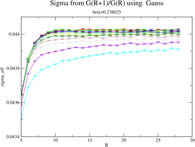
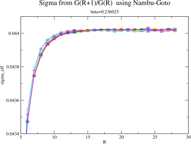
Figure 1: Effective string tension computed from $G(r+1)/G(r)$ using eq. (8). For $\beta=0.236025$, $L=80,50,40,30,28,26,24,22,20,18,16,14$. Upper plot: free field energy levels; lower plot: Nambu-Goto energy levels.

Looking at figures 2 and 3 we see that also for $\tilde{\beta}=0.24607$ and $\tilde{\beta}=0.27604$ the curves for different $L$ fall nicely on top of each other in the case of the Nambu-Goto ansatz, while there is a clear spread in the case of the free field ansatz. Finally, we notice that the $r$-dependence of $\sigma_{\mbox{\tiny{eff}}}$ is quite different for $\tilde{\beta}=0.27604$ compared with $\tilde{\beta}=0.24607$ and $\tilde{\beta}=0.236025$, i.e. there are sizable scaling corrections. From $L=60$ for $\tilde{\beta}=0.24607$ and $L=40$ for $\tilde{\beta}=0.27604$ and large values of $r$ we get $\sigma=0.082520(3)$ and $\sigma=0.20486(1)$ as our final estimate of the string tension at $\tilde{\beta}=0.24607$ and $\tilde{\beta}=0.27604$, respectively. The error quoted should include systematic errors. We get for the dimensionless combination $\sigma\xi^{2}=0.0933(4)$, $0.0893(4)$ and $0.0850(3)$ for $\tilde{\beta}=0.236025$, $0.24607$ and $0.27604$, respectively. The universal limit is given by $\lim_{\tilde{\beta}\rightarrow\tilde{\beta}_{c}}\sigma\xi^{2}=0.1056(19)$ [49].

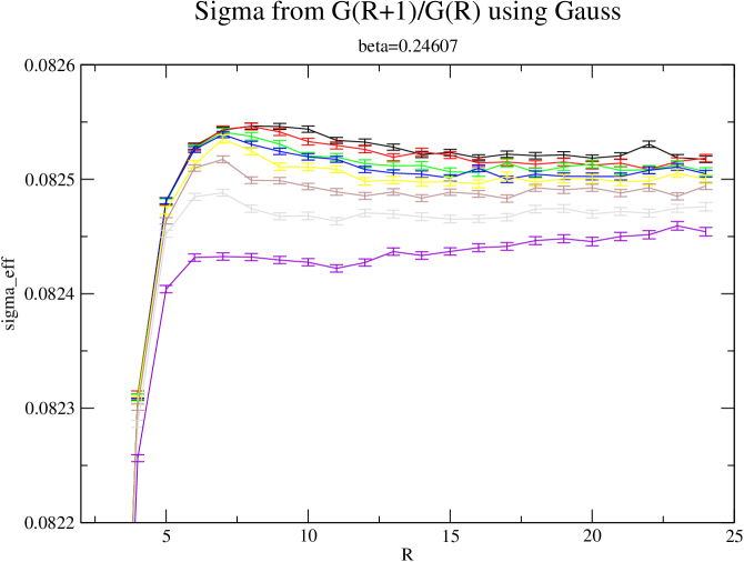
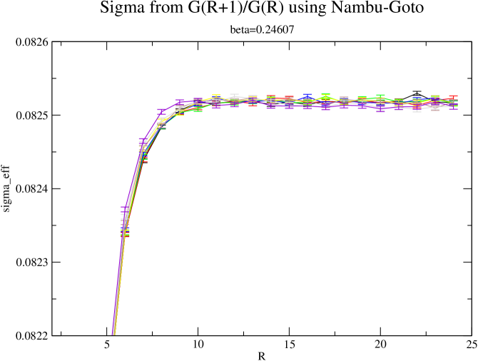
Figure 2: Effective string tension computed from $G(r+1)/G(r)$ using eq. (8) For $\tilde{\beta}=0.24607$, $L=60,30,24,22,20,18,16,14$. Upper plot: free field energy levels; lower plot: Nambu-Goto energy levels.

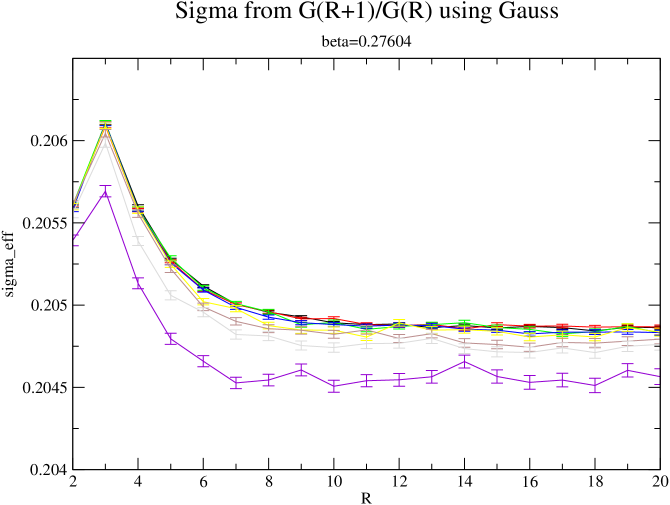
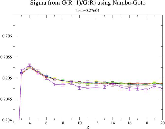
Figure 3: Effective string tension computed from $G(r+1)/G(r)$ using eq. (8) For $\beta=0.27604$, $L=40,30,20,16,14,12,10,8$. Upper plot: free field energy levels; lower plot: Nambu-Goto energy levels.

Finally in figure 4 we show $\sigma_{\mbox{\tiny{eff}}}$ obtained from $G(29)/G(28)$ at $\beta=0.236025$. For this particular value of $r$ we have added smaller values of $L$: $L=8,9,10,11,12$ and $13$. In the case of the Nambu-Goto energy-levels, $\sigma_{\mbox{\tiny{eff}}}$ is almost constant down to $L=14$, while for the free field energy levels there is a clear $L$ dependence in the same range of lattice sizes.

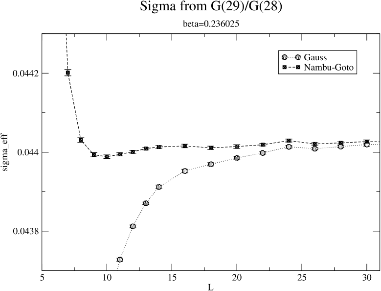
Figure 4: Effective string tension computed from $G(29)/G(28)$ using eq. (8) for $\beta=0.236025$. For Nambu-Goto and free field string states.

In figure 5 we have evaluated the effective string tension for $\tilde{\beta}=0.226102$ and $L=80$. The data are taken from table 3 of [15]. Our estimate of [14, 15] for the string tension is $\sigma=0.010560(18)$ and $\xi=3.09(1)$ for the correlation length, i.e. $\sigma\xi^{2}=0.1008(7)$. Similar to figure 1 for $\tilde{\beta}=0.236025$, we see for large $L$ that the Nambu-Goto matches the data less good than the free string prediction. This fact had also been pointed out in [15].

We may summarize the results of this first part of our analysis in the following two points:

• For all the values of $\beta$ that we studied the $L$ dependence of the interquark potential is well described by the Nambu-Goto effective string down to rather small values of $L$ (of the order of twice the deconfinement length). In this respect the Nambu-Goto string behaves much better than the simple free string model.

• String-related quantities (like the effective string corrections we are looking for) show much smaller scaling deviations than bulk observables. For instance, for the three values of $\beta$ that we studied, due to the very small values of $\xi$ the universal combination $\sigma\xi^{2}$ is still far from the continuum limit value, while in the same samples the $L$-dependence of the interquark potential is well described by the Nambu-Goto effective string (see the collapse of curves in figures 1 to 3), independently of the value of $\xi$.

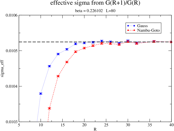
Figure 5: Effective string tension computed for $L=80$ using eq. (8) for $\tilde{\beta}=0.226102$. For Nambu-Goto and free field string states. Data taken from table 3 of [15].

4.1 The ground state energy

The ground state energy can be easily determined since, for large $L$, it dominates the string partition function:

$$Z_{\mbox{\tiny{spin}},Q\bar{Q}}(r,L)\simeq e^{-LE_{0}(r)}\;\;\;\;\;\;\mbox{for $L$ large}$$ (14)

In this limit, it is easy to make connection with the previous discussion:

$$\frac{G(r+1)}{G(r)}\simeq e^{-L[E_{0}(r+1)-E_{0}(r)]}\;\;\;\;\;\;\mbox{for $L$ large}$$ (15)

and, trivially

$$E_{0}(r)=\sum_{\tilde{r}=0}^{r-1}[E_{0}(\tilde{r}+1)-E_{0}(\tilde{r})]$$ (16)

Above we found for $\tilde{\beta}=0.236025$ and $L=80$ (where eq. (14) holds within our numerical precision for the whole range of $r$ considered) that $\sigma_{\mbox{\tiny{eff}}}$ (computed with the Nambu-Goto or the free field ansatz) for $r<10$ is clearly smaller than the asymptotic estimate of $\sigma$. It follows that also $E_{0}(r+1)-E_{0}(r)$ is clearly smaller than the Nambu-Goto and also the free field prediction, using the asymptotic estimate of $\sigma$. On the other hand, $\sigma_{\mbox{\tiny{eff}}}$ is constant within error-bars for the free field ansatz for $r>10$ and also for the Nambu-Goto ansatz starting from $r>15$ (where the difference of the Nambu-Goto and the free field theory prediction is smaller than the error of our Monte Carlo data).

It follows directly from eq. (16) that, due to the contributions from $r<10$, also for large values of $r$, $E_{0}(r)$ deviates from the effective string prediction (at least) by a constant.

In figure 6 we have plotted $E_{0}$ for $\tilde{\beta}=0.236025$ taken from the fit a.3 for $L_{\mbox{\tiny{min}}}=20$ discussed below. Note that $E_{0}$ is quite insensitive to the particular form of the fit and the value of $L_{\mbox{\tiny{min}}}$. We give $E_{0}(r)-E_{0,\mbox{\tiny{prediction}}}(r)-const$. $const$ is chosen such that $E_{0}(29)-E_{0,\mbox{\tiny{prediction}}}(29)-const=0$. For the theoretical prediction, we have taken $\sigma=0.044023$ obtained above. For this value of $\sigma$ we get $const\approx 0.16684$, for both NG and free field theory. For Nambu-Goto $E_{0}(r)-E_{0,\mbox{\tiny{NG}}}(r)-const$ is clearly larger than 0 for $r<18$. On the other hand, for the free field prediction, $E_{0}(r)-E_{0,\mbox{\tiny{free}}}(r)-const$ is slightly smaller than 0 for $9<r<20$, while it becomes positive for $r\leq 9$. Here one should note that for $\sigma=0.0440245$ instead, $E_{0}(r)-E_{0,\mbox{\tiny{free}}}(r)-const$ is consistent with zero for all $r\geq 10$.

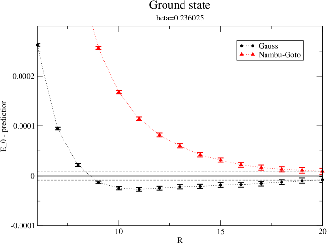
Figure 6: Ground state energy $E_{0}$ for $\tilde{\beta}=0.236025$ taken from the fit a.3 for $L_{\mbox{\tiny{min}}}=20$ discussed below. Note that $E_{0}$ is quite insensitive to the particular form of the fit and the value of $L_{\mbox{\tiny{min}}}$. The solid line indicates zero, the dashed lines indicate the error of $E_{0}(29)$ which enters the constant that has been subtracted. Note that the error in our estimate of the string tension $\sigma=0.044023(3)$ is not indicated in the figure.

4.2 The excited levels

From the free theory as well as from the Nambu-Goto effective string, we expect that the energy gaps $E_{n}-E_{0}$ are decreasing functions of the interquark distance $r$; in particular, for any $r_{0}$ and $n$ there exists an $r$ such that $E_{n}(r)-E_{0}(r)<E_{1}(r_{0})-E_{0}(r_{0})$. For such a choice of $r_{0}$, $r$ and $n$, we have:

$$G(r)/G(r_{0})=\exp\left(-[E_{0}(r)-E_{0}(r_{0})]L\right)\;\frac{\sum_{m=0}^{\infty}w_{m}\exp\left(-[E_{m}(r)-E_{0}(r)]L\right)}{\sum_{p=0}^{\infty}w_{p}\exp\left(-[E_{p}(r_{0})-E_{0}(r_{0})]L\right)}$$ (17)

$$= \exp\left(-[E_{0}(r)-E_{0}(r_{0})]L\right)\;\left[1+\sum_{m=1}^{n}w_{m}\exp\left(-[E_{m}(r)-E_{0}(r)]L\right)+\dots\right]$$

that is, the nontrivial $L$-dependence of $G(r)/G(r_{0})$ is dominated by the first $n$ states at the distance $r$, while the states at $r_{0}$ play virtually no role. Hence, a good matching of $G(\tilde{r}+1)/G(\tilde{r})$ with the NG prediction for $\tilde{r}>r_{0}$ implies that also the first few energy gaps at $r$ have to follow the NG prediction, and vice versa.

In the following, we determined the energy gaps from the correlation function $G(r)$. To this end, we performed a set of two- and three-parameter fits. Let us look at them in detail:

• two-parameter fits:

  • “Two-state” ansatz

    $$Z=e^{-E_{0}L}+e^{-E_{1}L}$$ (18)

    Here, the fit parameters are $E_{0}$ and $E_{1}$. This ansatz makes no use of the string-theory.

  • “Free-string” ansatz

    $$Z=\sum_{n=0}^{\infty}P(n)e^{-E_{n}L}$$ (19)

    with $E_{n}=E_{0}+n\Delta$, and $P(n)$ is the number of partitions of $n$; in this case, the fit parameters are $E_{0}$ and $\Delta$. Here we assume a string-spectrum as given by the free bosonic string. However, we allow $E_{0}$ and $\Delta$ to be independent.

  • “Nambu-Goto” ansatz

    $$Z=\sum_{n=0}^{\infty}P(n)e^{-E_{n}L}$$ (20)

    with $E_{n}=E_{0}+\Delta_{n}$, and $P(n)$ is the number of partitions of $n$. The energy-gaps $\Delta_{n}$ are given by eq. 6, where we allow for some $\sigma^{\prime}$, not related to the $E_{0}$ in the ansatz, i.e. the free parameters of the fit are $E_{0}$ and $\sigma^{\prime}$.

• three-parameter fits with:

  • “Three-state” ansatz

    $$Z=e^{-E_{0}L}+e^{-E_{1}L}+2e^{-E_{2}L}$$ (21)

    The fitted parameters are $E_{0}$, $E_{1}$ and $E_{2}$. Here, we have used the degeneracy of the second excited state as theoretical input.

  • “Modified free-string” ansatz

    $$Z=\sum_{n=0}^{\infty}P(n)e^{-E_{n}L}$$ (22)

    with: $E_{0}=a$, $E_{1}=a+b$, and $E_{n}=a+b+(n-1)c$ for $n>1$. In this case, the fitted parameters are $a$, $b$ and $c$. As in the fit of type a.2 we assume the linear rising of the energy levels typical of the free string, but allow the first energy gap (the parameter $b$ in the above equation) to behave independently of the remaining energy gaps.

The purpose of this choice is to distinguish between the “Nambu-Goto” and the free string behaviour.

In the following, we report the results for the sample at $\tilde{\beta}=0.236025$ which, according to the findings discussed in the previous section should be essentially unaffected by scaling violations as far as string-related quantities are concerned. In particular, we selected the results of the fits at four values of the interquark distance: $r=4,9,19,29$. As mentioned above, for this value of $\tilde{\beta}$ we run simulations corresponding to the following values of $L$: $L=80,50,40,30,28,26,24,22,20,18,16,14,13,12,11,10,9,8$. In the fits, only the data for $L_{\mbox{\tiny{min}}}\geq 14$ were included; then we studied the dependence of our results as $L_{\mbox{\tiny{min}}}$ was increased. Obviously, as $L$ is increased, the relative contribution of the ground state gets larger and larger, and higher states in the spectrum become negligible.

In table 1, we report the reduced $\chi^{2}$ of the fits and in figures 7 to 10 the best fit values for the lowest energy gap in the four cases.

Table 2 displays the number of excited states, which, according to our results at various values of $r$, lie below the glueball mass threshold; note that at short distances the glueball threshold is close to the lightest $E_{n}$ states.

Some comments on these results are in order.

• We expect that at large distance the Nambu-Goto string should describe the interquark potential well. This is indeed clearly visible if we look at the $r=29$ entries in table 1: the fits of type a.3 (Nambu-Goto) show small reduced $\chi^{2}$ values already for $L_{\mbox{\tiny{min}}}=14$, while fits of type a.1 and a.2 display a bad behaviour until large values of $L$ are reached, where the ground state dominates and only the first excited state gives further significant contributions. This is also clearly visible in figure 10 where the results for the energy gap of fit a.3 coincide with the Nambu-Goto prediction (the dashed line) already for $L_{\mbox{\tiny{min}}}=14$, while for the four other types of fit the data start for $L_{\mbox{\tiny{min}}}=14$ from values very far apart and smoothly converge toward the Nambu-Goto limit as $L_{\mbox{\tiny{min}}}$ increases. Notice that the combination of these two pieces of information (the reduced $\chi^{2}$ and the value of the $E_{1}-E_{0}$ gap as a function of $L_{\mbox{\tiny{min}}}$) tells us not only that the lowest gap agrees numerically with the NG expectation, but also that the whole spectrum must be of the NG type. In particular one should note that the difference between the NG behaviour (a.1 fit) and the free string one (a.2 fit) can be clearly distinguished by our data.

• A similar pattern also occurs for $r=19$, where, however, a systematic deviation with respect to the NG expectation for the energy gap starts to be visible. The data smoothly converge towards a value of the $E_{1}-E_{0}$ gap which is slightly larger than the NG expectation, though still very far from the free string one (solid line).

• For the two smallest values of $r$ the picture is completely different. All the fits behave equivalently well and the reduced $\chi^{2}$ cannot be used to distinguish among them. Also the best fit values for the energy gap essentially coincide (this is particularly visible in the $r=9$ case where all the symbols in figure 8 lie on top of each other). This indicates that in this case the data are not precise enough to detect higher states in the spectrum and only $E_{0}$ and $E_{1}$ play a role in the fits. This is not surprising, since, looking at eq. (6), we see that as $r$ decreases the energy gaps become larger and larger, making higher states negligible with respect to the two lowest ones. As in the $r=19$ case, we see a clear disagreement with respect to the NG expectation, the observed energy gap being larger than expected.

This disagreement is better appreciated in figure 11, in which we plotted the relative deviation of the first energy gap $E_{1}-E_{0}$ with respect to the free string prediction, as a function of the interquark distance. While the data are for all the values of $r$ very far from the free string expectation (solid line in the figure), they definitely disagree from the NG expectation for low values of $r$, and then nicely converge toward it as $r$ increases. The data for low values of $r$ perfectly agree with those reported in [22], where in fact a disagreement with respect to the NG picture was claimed. We confirm this disagreement at short distance, but being able to extend our analysis to larger values of $r$ we can confirm (in agreement with our previous observations [17]) that at large distances the NG picture, both in the quantitative value of the energy gap $E_{1}-E_{0}$ and in the general pattern of the excited states, is fully restored.

Another interesting feature of figure 11 is that it confirms the observation we made in the previous section, about the fact that string-related quantities (like the energy gap $E_{1}-E_{0}$) appear not to be strongly affected by scaling violations. In the figure we plot the data obtained for the three values of $\tilde{\beta}$ we studied, and — except for small deviations in the $\tilde{\beta}=0.276040$ case — the three samples nicely agree in the whole range of values of $r\sqrt{\sigma}$.

$r/a$	$L_{\mbox{\tiny{min}}}/a$	fit type a.1	fit type a.2	fit type a.3	fit type b.1	fit type b.2
4	14	000.97	00.97			0.83
	16	000.68	00.68
	18	000.33	00.33	0.33
	20	000.23	00.23
	22	000.27	00.27
	24	000.31	00.31
	26	000.38	00.38
9	14	005.77	03.40	1.63	01.84	1.73
	16	000.72	00.87	1.31	00.81
	18	000.72	00.75	0.84
	20	000.75	00.75	0.75
	22	000.87	00.86
	24	000.75	00.75
	26	000.90	00.90
	28	001.20
	30	001.80
	40	000.25
19	14			1.32		1.43
	16	227.19	13.35	0.90	01.26	0.87
	18	057.56	05.31	1.01	00.74
	20	019.02	03.45	1.14	00.82
	22	008.20	02.42		00.95
	24	000.82	00.35
	26	000.65	00.44
	28	000.29
	30	000.18
	40	000.36
29	14			1.21		2.01
	16		47.70	1.35		0.92
	18		22.57	1.51	15.19
	20		10.84	1.59	05.58
	22	171.38	05.08		02.74
	24	036.56	00.60		00.44
	26	016.68	00.75
	28	003.92
	30	002.39
	40	000.05

Table 1: Some details about the analysis of data at $\tilde{\beta}=0.236025$: the table shows the values of $\chi^{2}_{\mbox{\tiny{red}}}$ as a function of the minimum lattice size in the time-like direction, from the fits corresponding to the various ansätze discussed in subsection 4.2, and at different values of $r$.

$r/a$	# of states
4	1
9	3
14	4
19	5
24	6
29	7

Table 2: The number of excited $E_{n}$ states ($n\geq 1$) lighter than the glueball threshold, as a function of the interquark distance (in lattice units); the table shows the results obtained from simulations at $\tilde{\beta}=0.236025$.

Figure 7: Comparison of the results for the first energy gap $E_{1}-E_{0}$ obtained from different ansätze, as a function of the minimum value of $L$, at $\tilde{\beta}=0.236025$ for $r=4$.

Figure 8: Same as in previous figure, but for $r=9$.

Figure 9: Same as in previous figures, but for $r=19$.

Figure 10: Same as in previous figures, but for $r=29$.

Figure 11: Relative deviation of the first energy gap $E_{1}-E_{0}$, with respect to the free string prediction, as a function of the interquark distance; results are shown for different values of $\tilde{\beta}$, and are scaled in physical units. The format of this plot allows a direct comparison with figure 4 in [22].

5 Discussion and conclusions

The results of our analysis for the $\mathbb{Z}_{2}$ pure lattice gauge theory in $D=3$, which is expected to provide a prototypical model for quark confinement, show the following aspects.

1. A naïve description of the partition function associated with the confined $Q\bar{Q}$ sector of the theory expressed purely in terms of the standard effective string picture is not completely satisfactory, because the numerical results for the energy levels $E_{n}(r)$ do not agree with the corresponding theoretical spectrum, obtained by means of formal canonical quantisation of the Nambu-Goto string.

2. However, the observation that the differences $E_{0}(r+1)-E_{0}(r)$ are in agreement with the free string predictions for intermediate and large distances $r$, suggests that the deviations with respect to the string behaviour could be due to an overall shift in the spectrum induced by extra terms, which are relevant at short length scales, but negligible in the infrared limit.

3. Our numerical data confirm the Nambu-Goto string prediction for the energy gap $E_{1}(r)-E_{0}(r)$ for large interquark distances $r$. In particular, there is a large range in $r$, where the precision of our numerical results allows to clearly distinguish between the Nambu-Goto and the free string prediction and where we see a better agreement with the Nambu-Goto string than with its free string approximation.

4. Our fits indicate that also gaps $E_{n}(r)-E_{0}(r)$ with $n>1$ follow the Nambu-Goto prediction for sufficiently large $r$. Unfortunately, our data do not allow to make more quantitative statements on this issue.

Furthermore, we have discussed how the results on the spectrum that we have summarized above are related with the behaviour of the ratio $G(r+1)/G(r)$ of Polyakov loop correlation functions that we have analysed in previous studies [13, 14, 15, 16, 17]: A matching of $G(r+1)/G(r)$ with the Nambu-Goto string prediction for large $r$ implies that also the gaps $E_{n}(r)-E_{0}(r)$ follow the Nambu-Goto string prediction.

It is interesting to compare these results with other studies that are available in the literature; in particular, in [19, 20, 21, 22] the excitation spectrum was described in terms of the standard notation for the diatomic molecular physics, with states $\Gamma$ labelled by the component of the angular momentum of the gluon field along the interquark axis, and by the $CP$ eigenvalues. The numerical method they used to extract the lowest energy in the various $\Gamma$ sectors goes through evaluation of generalised Wilson loops, whose spatial edges were replaced by well-suited combinations of paths, transforming according to the quantum numbers of the considered $\Gamma$ state. They focused their study on a regime of intermediate distances, and the results show rather good agreement with the predictions of the adiabatic approximation of the bag picture [50], which provides a phenomenological model expected to interpolate between the short and long length scales; at large distances, however, the energies associated with the internal “gluonic” excitations of the stretched bag will become irrelevant to the lowest spectrum states, and a convenient description for the flux-tube will be given in terms of an effective string model. They also observe fine-structure deviations with respect to the $\frac{n\pi}{r}$ gaps expected from free-string model, that they compare with the Nambu-Goto spectrum (leaving room for the possibility that further physical effects can enter the effective string description in this regime).

In [23] a similar study was presented for the $SU(2)$ gauge model in $D=3$, concluding that the energy gaps at finite lattice spacing appear to be well modeled by the Nambu-Goto prediction, while the continuum extrapolation seems to favour the free string description.

As mentioned above, our results suggest instead that in the regime of intermediate to long distances the Nambu-Goto model (rather than the free-string one) correctly describes the spectrum of the theory, modulo an overall shift. As it concerns the interpretation of this shift, it is interesting to note that our analysis in the present work shows that major contributions to this effect come at distances smaller than the inverse of the mass of the lightest glueball: therefore, the shift in the energy levels likely depends on the gauge model which is considered and cannot be predicted in a pure string scenario. On the other hand, the fact that the differences $E_{0}(r+1)-E_{0}(r)$ appear to be better described by the free string than the Nambu-Goto one in a wide range of intermediate distances might be a (model-independent) effect due to the Liouville mode; the latter appears in the derivation of the Nambu-Goto effective model from the reparametrization invariant string theory in the framework of covariant quantization, and, due to its intractability, it must be neglected in the calculations yielding the effective string spectrum [31]. Neglecting the Liouville mode is allowed only in the critical dimension ($D=26$ for the Nambu-Goto string), in which it decouples from the theory. In the present $D=3$ case the field should not be neglected, however one can argue that the effect of this approximation becomes less and less important as the interquark distance increases — a scenario which indeed appears to be compatible with our numerical results.

It would be very interesting to extend the present study to other models (especially to different values of $D$, which gives the coupling of the Liouville mode) to see if the present picture is confirmed, and to identify how the deviations from the Nambu-Goto effective string depend on the gauge group and on the number of space-time dimensions.

Acknowledgements. This work was partially supported by the European Commission TMR programme HPRN-CT-2002-00325 (EUCLID). M. P. acknowledges support received from Enterprise Ireland under the Basic Research Programme.

References

- [1] M. Lüscher, K. Symanzik and P. Weisz, Nucl. Phys. B 173 (1980) 365.
- [2] M. Lüscher, G. Münster and P. Weisz, Nucl. Phys. B 180 (1981) 1.
- [3] M. Lüscher, Nucl. Phys. B 180 (1981) 317.
- [4] O. Alvarez, Phys. Rev. D 24 (1981) 440.
- [5] R. D. Pisarski and O. Alvarez, Phys. Rev. D 26 (1982) 3735.
- [6] K. Dietz and T. Filk, Phys. Rev. D 27 (1983) 2944.
- [7] J. F. Arvis, Phys. Lett. B 127 (1983) 106.
- [8] J. Ambjorn, P. Olesen and C. Peterson, Nucl. Phys. B 244 (1984) 262.
- [9] P. Olesen, Phys. Lett. B 160 (1985) 144.
- [10] P. Olesen, Phys. Lett. B 160 (1985) 408.
- [11] J. Polchinski and A. Strominger, Phys. Rev. Lett. 67 (1991) 1681.
- [12] M. Lüscher and P. Weisz, JHEP 0407 (2004) 014 [arXiv:hep-th/0406205].
- [13] M. Caselle, M. Panero and P. Provero, JHEP 0206 (2002) 061 [arXiv:hep-lat/0205008].
- [14] M. Caselle, M. Hasenbusch and M. Panero, JHEP 0301 (2003) 057 [arXiv:hep-lat/0211012].
- [15] M. Caselle, M. Hasenbusch and M. Panero, JHEP 0405 (2004) 032 [arXiv:hep-lat/0403004].
- [16] M. Caselle, M. Pepe and A. Rago, JHEP 0410 (2004) 005 [arXiv:hep-lat/0406008].
- [17] M. Caselle, M. Hasenbusch and M. Panero, JHEP 0503 (2005) 026 [arXiv:hep-lat/0501027].
- [18] T. J. Allen, M. G. Olsson and S. Veseli, Phys. Lett. B 434 (1998) 110 [arXiv:hep-ph/9804452].
- [19] K. J. Juge, J. Kuti and C. Morningstar, Phys. Rev. Lett. 90 (2003) 161601 [arXiv:hep-lat/0207004].
- [20] K. J. Juge, J. Kuti and C. Morningstar, Nucl. Phys. Proc. Suppl. 129 (2004) 686 [arXiv:hep-lat/0310039].
- [21] K. J. Juge, J. Kuti and C. Morningstar, arXiv:hep-lat/0312019.
- [22] K. J. Juge, J. Kuti and C. Morningstar, arXiv:hep-lat/0401032.
- [23] P. Majumdar, arXiv:hep-lat/0406037.
- [24] G. Bali, arXiv:nucl-th/0410080.
- [25] Y. Nambu, in “Symmetries and Quark Models”, ed. R. Chand (Gordon and Breach, New York, 1970).
- [26] T. Goto, Prog. Theor. Phys. 46 (1971) 1560.
- [27] Y. Nambu, Phys. Rev. D 10 (1974) 4262.
- [28] P. Goddard, J. Goldstone, C. Rebbi and C. B. Thorn, Nucl. Phys. B 56, 109 (1973).
- [29] M. B. Green, J. H. Schwarz, E. Witten, “Superstring Theory”, Vol. 1 (Cambridge University Press, Cambridge, 1988).
- [30] J. Polchinski, “String Theory”, Vol. 1 (Cambridge University Press, Cambridge, 1998).
- [31] M. Billó and M. Caselle, arXiv:hep-th/0505201.
- [32] J. M. Drummond, arXiv:hep-th/0411017.
- [33] Y. Deng and H. W. J. Blöte, Phys. Rev. E 68 (2003) 036125.
- [34] M. Hasenbusch and K. Pinn, J. Phys. A 30 (1997) 63 [arXiv:cond-mat/9605019].
- [35] M. Caselle, M. Hasenbusch, P. Provero and K. Zarembo, Nucl. Phys. B 623 (2002) 474 [arXiv:hep-th/0103130].
- [36] M. Hasenbusch and K. Pinn, Physica A 203 (1994) 189 [arXiv:hep-lat/9310013].
- [37] M. Caselle, R. Fiore, F. Gliozzi, M. Hasenbusch, K. Pinn and S. Vinti, Nucl. Phys. B 432 (1994) 590 [arXiv:hep-lat/9407002].
- [38] K. Rummukainen, Nucl. Phys. B 390 (1993) 621 [arXiv:hep-lat/9209024].
- [39] P. de Forcrand, M. D’Elia and M. Pepe, Phys. Rev. Lett. 86 (2001) 1438 [arXiv:hep-lat/0007034].
- [40] P. de Forcrand, M. D’Elia and M. Pepe, Nucl. Phys. Proc. Suppl. 94 (2001) 494 [arXiv:hep-lat/0010072].
- [41] M. Pepe and P. De Forcrand, Nucl. Phys. Proc. Suppl. 106 (2002) 914 [arXiv:hep-lat/0110119].
- [42] M. Caselle, R. Fiore, F. Gliozzi, M. Hasenbusch and P. Provero, Nucl. Phys. B 486 (1997) 245 [arXiv:hep-lat/9609041].
- [43] M. Panero, JHEP 0505 (2005) 066 [arXiv:hep-lat/0503024].
- [44] M. Caselle and M. Hasenbusch, Nucl. Phys. B 470 (1996) 435 [arXiv:hep-lat/9511015].
- [45] M. Caselle and M. Hasenbusch, J. Phys. A 30 (1997) 4963 [arXiv:hep-lat/9701007].
- [46] M. Caselle, M. Hasenbusch and P. Provero, Nucl. Phys. B 556, 575 (1999) [arXiv:hep-lat/9903011].
- [47] H. Arisue and K. Tabata, Nucl. Phys. B 435 (1995) 555 [arXiv:hep-lat/9407023].
- [48] M. Campostrini, A. Pelissetto, P. Rossi and E. Vicari, Phys. Rev. E 57 (1998) 184 [arXiv:cond-mat/9705086].
- [49] V. Agostini, G. Carlino, M. Caselle and M. Hasenbusch, Nucl. Phys. B 484 (1997) 331 [arXiv:hep-lat/9607029].
- [50] T. DeGrand, R. L. Jaffe, K. Johnson and J. E. Kiskis, Phys. Rev. D 12 (1975) 2060.