Simulations in Early Universe Theory

Abstract:

We give an impression of the type of results that have been obtained with numerical lattice simulations of field theory in the early universe.

PoS(LAT2005)022

1 Introduction

When indicating various transitions that are supposed to have taken place in the early universe [1] on a time line (Fig. 1),

Figure 1: Transitions in the early universe. Going backwards in time there was the decoupling of photons (DEC), observed today as the Cosmological Microwave Background, a point of equal energy in ‘radiation’ and (non-relativistic) ‘matter’ (EQ), a period of nucleosynthesis (NS), probably a QCD transition, and presumably an ElectroWeak transition. There are good arguments for a period of inflation, with support from the microwave background. When inflation ended is uncertain. Leptogenesis (LG) and/or baryogenesis (BG) is supposed to have taken place after inflation and before or during the EW transition.

one is confronted by the fact that what we know with confidence goes back only to the time of nucleosynthesis. Was there a QCD transition? Probably, because its temperature of 150 MeV is only two orders of magnitude higher than that at the start of nucleosynthesis. The temperature of the conventional electroweak transition is already three orders of magnitude higher than that of the QCD transition. Could it have been different? Where should one put the end of inflation, baryogenesis? To make progress we need to understand as much as possible of the dynamical behavior of a universe, given our knowledge of fundamental interactions. This often concerns non-perturbative phenomena.

This talk is about numerical simulations in field theory, for early times, around and before the supposed electroweak transition, using lattice regularization. We will give an impression by examples of what has been done, it is not a review.

2 Inflation, preheating, defects, baryogenesis, thermalization

Let us take a brief look at various topics in the title of this section.

Inflation

Simple models [2] are formulated in terms of an inflaton field, $\sigma$, the Friedmann-Lemaître-Robertson-Walker scale factor $a$, which satisfy the dynamical equations

$$0 = \ddot{\sigma}+3H\dot{\sigma}-\frac{\nabla^{2}\sigma}{a^{2}}+\frac{\partial V(\sigma,\cdots)}{\partial\sigma},$$

$$H\equiv\frac{\dot{a}}{a} = \sqrt{\frac{\rho}{3m_{\rm P}^{2}}},$$

$$\rho = \frac{\dot{\sigma}^{2}}{2}+\frac{(\nabla\sigma)^{2}}{2a^{2}}+V(\sigma,\cdots)+\cdots$$

in flat space. Here $H$ is the Hubble rate and $\rho$ the energy density. When the potential energy of the inflaton dominates and its potential is very flat, there is strong damping and ‘slow roll’, a nearly constant Hubble rate and approximately exponential expansion $a\propto e^{Ht}$. Inflaton models can be divided into two classes: small-field and large-field models (Fig. 2), depending on $\sigma$ rolling away or towards the origin, respectively. Other names are ‘new inflation’ and ‘chaotic inflation’, respectively.

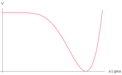
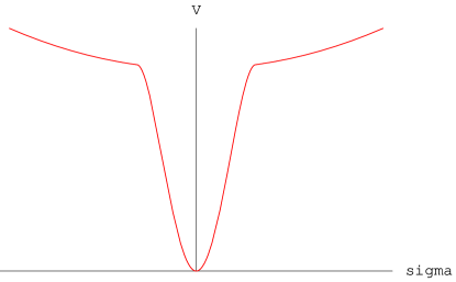
Figure 2: Small-field (left) and large-field (right) inflaton potentials.

The large-field potential shown in Fig. 2 (right) is an example of a so-called hybrid-inflation model:

$$V(\sigma,\varphi)=V_{0}+\frac{1}{2}\,\mu_{\sigma}^{2}\sigma^{2}+g^{2}\sigma^{2}\varphi^{\dagger}\varphi-\mu^{2}\varphi^{\dagger}\varphi+\lambda(\varphi^{\dagger}\varphi)^{2},$$ (1)

where $\varphi$ could be a Higgs field. Flatness of the potential requires relatively small $\mu_{\sigma}$, typically $\mu_{\sigma}\ll\mu$. During inflation the inflaton field is large, $g^{2}\sigma^{2}-\mu^{2}>0$ and $\varphi=0$ (read $\langle\varphi\rangle=0$). Inflation ends when $g^{2}\sigma^{2}-\mu^{2}$ goes negative. Assuming the $\varphi$ dynamics to be much faster than that of the inflaton, we can solve for $\varphi^{\dagger}\varphi$ and substitute it back into the potential: $\varphi^{\dagger}\varphi\to(\mu^{2}-g^{2}\sigma^{2})/\lambda$. This gives the trough near the origin shown in the right plot of Fig. 2 (a similar substitution has been assumed in the left plot). When the inflaton has gone down the ‘waterfall’, the universe is assumed to be cold and without appreciable baryon- and lepton-number densities, because it has just undergone a huge expansion. The energy in the inflaton has to be transferred to other degrees of freedom (d.o.f.) in order for baryogenesis to become possible, such that it ends up eventually at the standard hot radiation-dominated stage during nucleosynthesis. This heating up (called ‘re-heating’) might take too long in a given model, but non-perturbative pre-heating processes may have helped to achieve it.

Preheating

Rewriting the potential in the form $V(\sigma,\cdots)=V(\sigma)+(g^{2}\sigma^{2}-\mu^{2})\varphi^{\dagger}\varphi+\cdots$ reveals an effective $\varphi$ mass parameter,

$$\mu_{\rm eff}^{2}=-\mu^{2}+g^{2}\sigma^{2}.$$

Its time dependence can have drastic non-perturbative effects:

$\cdot$ $\langle\sigma\rangle$ oscillates $\to$ $\varphi$ resonates [4];

$\cdot$ $\mu_{\rm eff}^{2}<0$ $\to$ tachyonic instability [5].

Also the $\sigma$ modes can resonate and $\sigma$ is also tachyonic during the time that $\partial^{2}V/\partial\sigma^{2}<0$. These non-perturbative effects can result in large occupation numbers of $\sigma$ and $\varphi$, in a limited momentum range. Such processes are called pre-heating.

Defects

Preheating processes often result in the formation of defects, depending on the fields involved:

• domain walls, strings, monopoles (see e.g. [1]), textures [6], Q-balls, I-balls, oscillons (see e.g. [7, 8]), half-knots, Chern-Simons number-densities, …

They may play a role in baryogenesis, thermalization and structure formation.

Baryogenesis

The aim is to explain the baryon to photon ratio $n_{B}/n_{\gamma}\simeq 6.5\,10^{-10}$ from $n_{B}=0$ (inflation) and B-number, C & CP violation, during particle physics processes out of equilibrium. Many scenarios for doing this have been proposed, see e.g. [9, 10]. Here we shall focus on one for which lattice simulations have been carried out: Cold ElectroWeak Baryogenesis [11, 12, 13, 14, 15].

In this scenario one assumes that the electroweak transition was tachyonic of the type discussed below (1), and occurred at the end of a period of inflation when the universe was still cold (so the electroweak transition was not caused by the falling temperature of the universe.) The electro-weak anomaly in the baryon current

$$\partial_{\mu}j^{\mu}_{B}=3\,q,\quad q=\frac{1}{16\pi^{2}}\,\mbox{tr}F_{\mu\nu}\tilde{F}^{\mu\nu}$$

with $q$ the ‘topological-charge’ density of the $SU(2)$ gauge field, can be integrated over the transition to give a baryon asymmetry

$$B(t)=3\int_{0}^{t}dt^{\prime}\,\int d^{3}x\,\langle q({\bf x},t^{\prime})\rangle.$$ (2)

This can be non-zero because the tachyonic transition occurred under the influence of C and CP violation.

Thermalization

The important question is: how long does it take to thermalize the expanding universe after inflation? The ‘re-heating’ temperature $T_{\rm rh}$ marks the beginning of the radiation-dominated universe. Nucleosynthesis constrains this to $T_{\rm rh}\gtrsim 4$ MeV [16]. Thermalization is a non-perturbative problem in out-of-equilibrium quantum field theory.

3 Classical approximation

Non-perturbative computations of expectation values observables like

$$\langle O(t)\rangle=\mbox{Tr}\,\rho\,O(t)=\mbox{Tr}\,\rho\,U^{\dagger}(t)\,O\,U(t)$$

where $\rho$ is the density operator and $U(t)$ is the evolution operator in real time, are very difficult in quantum field theory. The classical approximation can therefore be very useful, since it is possible to solve the fully non-linear field equations on a computer (a perturbative analysis is given in [17, 18]). To formulate this we can think of a coherent state [19] or Wigner representation [20]

$$\langle O(\phi,\pi)\rangle=\int D\phi_{\rm c}\,D\pi_{\rm c}\,\rho_{\rm c}(\phi_{\rm c},\pi_{\rm c})\,O(\phi_{\rm c},\pi_{\rm c})$$

where $\phi_{\rm c}$ and $\pi_{\rm c}$ are classical conjugate variables. If, under suitable conditions, the functional $\rho_{\rm c}$ is positive (generally not true in the quantum regime), then we can use it as a probability for initial conditions. The classical approximation then goes as follows:

1. draw an initial configuration from $\rho_{\rm c}(\phi_{\rm c},\pi_{\rm c})$
2. solve classical e.o.m. for $\phi_{\rm c}$ and $\pi_{\rm c}$
3. evaluate $O(\phi_{\rm c},\pi_{\rm c})$
4. average over initial configurations

One expects a classical approximation to be applicable in cases where large occupation numbers dominate, which depends on the observable and on the initial conditions. Let us take a look at occupation numbers. For a free scalar field the usual definition is

$$n_{\bf k}=\langle a_{\bf k}^{\dagger}a_{\bf k}\rangle,\quad a_{\bf k}=\frac{1}{\sqrt{2\omega_{\bf k}}}(\omega_{\bf k}\phi_{\bf k}+i\pi_{\bf k}),$$

where $\phi_{\bf k}$ and $\pi_{\bf k}$ are Fourier modes of the canonical variables, and $\omega_{k}$ is the corresponding energy ($\sqrt{k^{2}+m^{2}}$). We can generalize this to time-dependent quasi-particle energies $\omega_{\bf k}$ and occupation numbers $n_{\bf k}$, $\tilde{n}_{\bf k}$, defined by

$$\langle\phi_{\bf k}\phi_{\bf k}^{\dagger}\rangle\equiv\left(n_{\bf k}+\frac{1}{2}\right)\frac{1}{\omega_{\bf k}},\quad\langle\pi_{\bf k}\pi_{\bf k}^{\dagger}\rangle\equiv\left(n_{\bf k}+\frac{1}{2}\right)\omega_{\bf k},\quad\langle\phi_{\bf k}\pi_{\bf k}^{\dagger}\rangle\equiv\tilde{n}_{\bf k}+\frac{i}{2}.$$ (3)

Given the correlation functions, we can easily solve for $\omega_{\bf k}$, $n_{\bf k}$ and $\tilde{n}_{\bf k}$, and see if $n_{\bf k}$ and $\tilde{n}_{\bf k}$ are larger than 1.

Consider now a tachyonic transition at $t=t_{c}$, when $\mu_{\rm eff}^{2}(t_{c})=0$. Assume that the couplings are weak enough that a gaussian approximation makes sense. The e.o.m. for a component of $\varphi$ is then

$$\ddot{\phi}_{\bf k}+(\mu_{\rm eff}^{2}+k^{2})\phi_{\bf k}=0.$$

Two cases for which this equation can be solved are [21, 22]

$$\mu_{\rm eff}^{2}=-M^{3}(t-t_{c}),\quad M^{3}\equiv-2g^{2}\,\sigma_{c}\dot{\sigma}_{c},$$ (4)

valid near $t_{c}$, and the sudden quench [23]

$$\mu_{\rm eff}^{2} = +\mu^{2},\quad t<t_{c},$$ (5)

$$= -\mu^{2},\quad t>t_{c}.$$ (6)

One finds that $n_{k}$ and $\tilde{n}_{k}$ grow faster than exponential and $n_{k}+1/2-\tilde{n}_{k}\to 0$, for $k<k_{\rm max}$:

$$k_{\rm max} = \sqrt{M^{3}(t-t_{c})}$$ (7)

$$= \mu,\quad\mbox{for the quench.}$$ (8)

Quantum $\langle\cdots\rangle$ dominated by the growing modes can after some time be well reproduced by the classical distribution

$$\exp\left[-\frac{1}{2}\sum_{k\leq k_{\rm max}}\left(\frac{|\xi^{+}_{\bf k}|^{2}}{n_{k}+1/2+\tilde{n}_{k}}+\frac{|\xi^{-}_{\bf k}|^{2}}{n_{k}+1/2-\tilde{n}_{k}}\right)\right],\quad\xi^{\pm}_{{\bf k}}=\frac{1}{\sqrt{2\omega_{k}}}\left(\omega_{k}\,\phi_{{\bf k}}\pm\pi_{\bf k}\right).$$ (9)

The condition $k\lesssim k_{\rm max}$ can be relaxed provided that the high-momentum modes can be dealt with by renormalization.

So for tachyonic transitions we obtain well motivated initial conditions for a classical approximation:

1a. at time $t_{\rm i}>t_{c}$ when $n_{k},\tilde{n}_{k}\gg 1$ and non-linear terms in the e.o.m. are still small
1b. (‘just the half’) alternatively, choose $t_{\rm i}=t_{c}$
2. choose between $k_{\rm max}$ as in (7) or (8), or $k_{\rm max}=$ ‘cutoff’ (all modes)
3. draw the initial $\phi$ and $\pi$ from the gaussian ensemble (9)

The alternative 1b. is possible because quantum and classical evolution are formally identical for a free field. The initial particle numbers are zero in this case, so in (9), $n_{k}+1/2\pm\tilde{n}_{k}=1/2$ whence the name ‘just the half’ [23]. In case of $k_{\rm max}\neq$ ‘cutoff’, the initial modes with $k>k_{\rm max}$ are set to zero. Proposals of this kind appeared earlier in the literature [20] (see also [24]).

An attractive formulation for numerical simulations is obtained by first discretizing the action on a space-time lattice, with spacings $a_{t}\ll a_{s}$, and then deriving the field equations from the stationary action principle. This especially useful for gauge fields [25], and it leads to leapfrog-type e.o.m. Some milestones in early universe simulations are the computation of the sphaleron rate at high temperature [26, 27], and the unveiling of ‘re-scattering’ effects after parametric resonance [28] and tachyonic preheating [5]. In the following some examples will be mentioned of more recent work.

Figure 3: Inflaton occupation numbers $n_{k}$ at various times. A resonance is visible at $t=876$ ($t$ and $k$ in $\sqrt{\lambda}v$-units). From [29].

Example: particle numbers in ‘New inflation’ [29]

The inflaton potential is a small field model of the Coleman-Weinberg form

$$V(\sigma)=\frac{1}{4}\,\lambda\sigma^{4}\left(\ln\frac{|\sigma|}{v}-\frac{1}{4}\right)+\frac{1}{16}\,\lambda v^{4}.$$

Using an equilibrium one-loop potential for non-equilibrium dynamics is questionable, in principle, but it may be justifiable by assuming relatively fast dynamics for the non-inflaton d.o.f. The parameters are $\lambda=10^{-12}$, $v=10^{-3}\,m_{\rm P}$ ($m_{\rm P}$ is the Planck mass), typical values for satisfying the CMB constraints. The simulation takes the Hubble expansion into account. Initially $\langle\sigma\rangle\approx 0$, after inflation it rolls into minimum of $V$ where it oscillates, the energy decays into $\sigma$-particles. Figure 3 (left) shows how inflaton particle-numbers have become very large due to tachyonic preheating, and one can see also parametric resonance around time 876.

By including another field $\phi$ the transfer of energy to other d.o.f. is studied. The potential is taken as $V=V(\sigma)+\frac{1}{2}\,g^{2}\sigma^{2}\phi^{2}$. This is non-tachyonic for $\phi$ – the $\phi$ particle numbers grow exponentially because of parametric resonance. Figure 3 (right) shows the number densities $n=\int\frac{d^{3}k}{(2\pi)^{3}}\,n_{k}$ for the two species, for two values of the couplings. The resonance is more efficient for smaller $g^{2}$, but $n_{\phi}\ll n_{\sigma}$ and the inflaton does not loose its energy very fast. So in this case preheating is not very efficient and the reheating temperature is estimated analytically to be $T_{\rm rh}\approx\sqrt{m_{\rm P}\,\Gamma_{\mbox{}\!\sigma\to\phi\phi}}$ ($\approx 10^{7}$ GeV for $g^{2}\lesssim\lambda$).

Example: mixing in an inflaton–SU(2)-Higgs model [22]

The potential corresponds to a large-field model

$$V=\textstyle{\frac{1}{2}}\,\mu_{\sigma}^{2}\sigma^{2}+g^{2}\sigma^{2}\varphi^{\dagger}\varphi+\lambda\left(\varphi^{\dagger}\varphi-\textstyle{\frac{1}{2}}\,v^{2}\right)^{2},$$ (10)

in which the inflaton is coupled to the Higgs sector of the Standard Model, albeit with somewhat unrealistic couplings, $\lambda=0.11/4$, $g^{2}=2\lambda$. The Hubble expansion is negligible for $v=246$ GeV ($H=O(10^{-14})$ GeV). The initial conditions where drawn from a fit to the $k$-dependence of the distribution at $t=t_{\rm i}$, with $M=0.18\,m$, $m=\sqrt{\lambda}\,v$ (cf. (4)). Figure 4 shows the Higgs field in an $x$-$y$ slice through the lattice at various times after the transition. Intuitively, the non-linear scattering of waves causes a good mixing of field modes and shortens the period needed to reach the thermalized state.

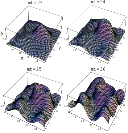
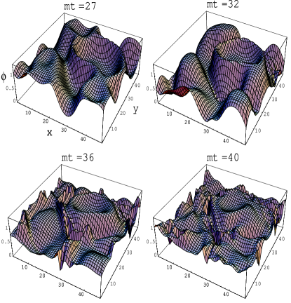
Figure 4: Higgs-field amplitude in $x$-$y$ slice at various times. From [22].

Example: equation of state in an inflaton–U(1)-scalar model [30]

The equation of state (e.o.s.), i.e. $p=p(\rho)$, is a basic ingredient in hydrodynamic descriptions of the early universe. In simple descriptions the cosmic fluid is often approximated by mixture of various contributions, such as ‘radiation’ $p=\rho/3$, ‘matter’ $p\simeq 0$, ‘vacuum’ $p=-\rho$, and it is interesting to see if and when such an approximation makes sense. The potential in this study is the U(1) version of (10). The energy scale is presumed much higher in this case, with parameters $g^{2}=10^{-2}$, $\lambda=g^{2}/2$, $\mu_{\sigma}=4\,10^{11}$ GeV, $m_{\rm H}=\sqrt{2}\,m=9\,10^{14}$ GeV. There are no gauge fields. The Hubble expansion is taken into account. Writing

$$\varphi=r\,e^{i\alpha}$$

the pressures of the inflaton, Higgs and Goldstone bosons are defined as

$$p_{\rm H} = \textstyle{\frac{1}{2}}\,\dot{r}^{2}-\textstyle{\frac{1}{6}}\,(\nabla r/a)^{2}+\textstyle{\frac{1}{4}}\,\lambda(r^{2}-v^{2})^{2},$$

$$p_{\rm G} = \textstyle{\frac{1}{2}}\,r^{2}\dot{\alpha}^{2}-\textstyle{\frac{1}{6}}(\nabla\alpha/a)^{2},$$

$$p_{\sigma} = \textstyle{\frac{1}{2}}\,\dot{\sigma}^{2}-\textstyle{\frac{1}{6}}(\nabla\sigma/a)^{2}+\textstyle{\frac{1}{2}}\,(\mu_{\sigma}^{2}+g^{2}r^{2})\sigma^{2}.$$

Figure 5 shows the emergence of an equation of state and its break-up into various contributions. We see how the Goldstone modes approach the radiation e.o.s. $p=\rho/3$, whereas the massive Higgs and inflaton modes clearly differ from this. The complete pressure is the sum of these components and this study indicates that a definite e.o.s. emerges around $tm\approx 85$ after the transition. Some of the contributions were interpreted in terms of global strings [30].

Figure 5: Parametric plot of the pressures $p_{\rm H}$, $p_{\rm G}$ and $p_{\sigma}$ vs the energy density $\rho$, for times $tm=85-200$, and two lattice spacings, $a_{s}m=0.5$, 1. From [30].

Example: strings and hot spots [31]

Global strings are an example of (unstable) topological defects which one expects to be produced in a tachyonic transition, and which may be relevant for elucidating the mechanism of tachyonic pre-heating. Other possible objects of interest are ‘hot spots’, places where the inflaton field has ‘jumped’ over the trough in Fig. 2 (right) and ends up again at values $|\sigma|>\sigma_{c}$. The model is the same U(1) inflaton-‘Higgs’ model as in the previous example (with $v^{2}/2\to v^{2}$). The parameters are $g^{2}=10^{-4}$, $\lambda=10^{-2}$, $m\equiv\sqrt{2\lambda}\,v=3\,10^{15}$ GeV, and the expansion rate is taken to have the constant value $H=3.6\,10^{-3}\,m$. The initialization is at $\sigma=\sigma_{c}$ when $\mu_{\rm eff}^{2}\equiv g^{2}\sigma^{2}-m^{2}=0$, à la ‘just the half’ with $k_{\rm max}$ = ‘cutoff’.

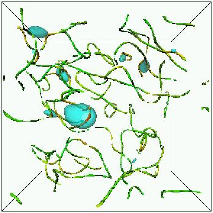
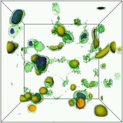
Figure 6: Left: transparent surface: $\sigma=-\sigma_{c}$ at time $tm=130$; strings: $|\varphi|^{2}=v^{2}/10$ at time for which spatial average $\overline{\sigma}=0$ for the first time. Right: transparent green surface: $|\varphi|^{2}=v^{2}/10$; blue: $\sigma=\sigma_{c}$; yellow: $\sigma=-\sigma_{c}$; time $tm=270$. From [31].

Figure 6 shows surfaces where $\sigma$ has fluctuated to $\pm\sigma_{c}$, and tubes of $|\varphi|^{2}=v^{2}/10$, inside of which the centers of strings are located at $\varphi=0$. At the later time $tm=270$ the strings have mostly decayed, but not the ‘hot spots’. The authors of [31] remark that the hot spots play an important role in the efficiency of tachyonic preheating.

Example: Tachyonic electroweak quench [32]

The emergence and development of particle distribution functions in a tachyonic electroweak transition has been studied with the SU(2)-Higgs model

$$-{\cal L}_{\rm SU(2)H}=\frac{1}{2g^{2}}\,\mbox{tr}F_{\mu\nu}F^{\mu\nu}+(D_{\mu}\varphi)^{\dagger}D^{\mu}\varphi-\mu^{2}\varphi^{\dagger}\varphi+\lambda(\varphi^{\dagger}\varphi)^{2},$$

with fairly realistic couplings, $m_{W}=82$ GeV, $m_{\rm H}/m_{W}=\sqrt{2}$. The initial conditions for the Higgs field were taken to be the quench (6), ‘just the half’, with $k_{\rm max}=\mu=m_{\rm H}/\sqrt{2}=0.25/a_{s}$. The initial gauge field potentials ${\bf A}$ were set to zero (since they are on the same footing as $\varphi_{\bf k}$ with $k>k_{\rm max}$), and the canonical conjugates $\dot{\bf A}$ then followed from the Gauss constraint in the temporal gauge (${\bf A}_{0}=0$) used for solving the e.o.m. The particle distribution functions $n_{k}$ for the Higgs and gauge fields were computed as in (3), after fixing the gauge to ‘Coulomb’ or ‘unitary’.

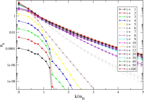
(11)

Figure 7: Coulomb-gauge W-particle numbers as a function of momentum, time in units of $m_{H}^{-1}$. From [32].

Figure 7 shows the development of the $W$-particle numbers. At first the low-momentum modes increase exponentially fast due to their coupling to the unstable Higgs modes. At time 7 there is a change of behavior in the tail of the distribution. Approximate thermalization was found to set in from $tm_{\rm H}=30$ or so onwards, and not much happened in $50\lesssim tm_{\rm H}<100$. At $tm_{\rm H}=100$ there is approximate gauge-independence in the transverse $W$-particle numbers, but the longitudinal $W$-modes settle at a slower rate. Effective Higgs and $W$ temperatures at that time agreed reasonably well. Effective chemical potentials $\mu_{\rm chem}\approx 0.7$ (0.9) for $W$ (H) are expected to vanish much later.

Example: Cold electroweak baryogenesis [15, 33]

In this simulation the scenario was tested using an effective CP-violating term in the equations of motion following from the lagrangian

$${\cal L}={\cal L}_{\rm SU(2)H}-\frac{3\delta}{m_{W}^{2}}\,\varphi^{\dagger}\varphi\,q,\quad q=\frac{1}{16\pi^{2}}\,\mbox{tr}\,F_{\mu\nu}\tilde{F}^{\mu\nu}.$$

Here 3 is the number of families and $\delta$ parametrizes effective CP violation, perhaps from physics beyond the Standard Model. Since $q$ is a total derivative, $q=\partial_{\mu}j^{\mu}_{\rm CS}$, it is customary to rewrite the anomaly equation (2) in the form

$$B(t)=3\langle N_{\rm CS}(t)-N_{\rm CS}(0)\rangle,$$

with $N_{\rm CS}=\int d^{3}x\,j^{0}_{\rm CS}$ the Chern–Simons number. A useful parameter is furthermore $N_{\rm w}$, the winding number of the Higgs field, since $N_{\rm CS}\approx N_{\rm w}$, is expected to hold when fluctuations have sufficiently diminished. The parameters of the simulation were $m_{W}=82$ GeV, $m_{\rm H}/m_{W}=1$, $\sqrt{2}$, $\sqrt{3}$ and 2, quench initial conditions with $k_{\rm max}=\mu$. The lattice implementation of CP violation leads to implicit e.o.m. which were solved by iteration at a substantially increased time of computation.

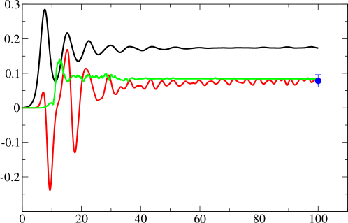
Figure 8: $\langle\varphi^{\dagger}\varphi\rangle$(black), $\langle N_{\rm CS}\rangle$(red), $\langle N_{\rm w}\rangle$(green) vs time in units $m_{\rm H}^{-1}$; $\delta=1$, $m_{\rm H}=\sqrt{2}\,m_{W}$. From [33].

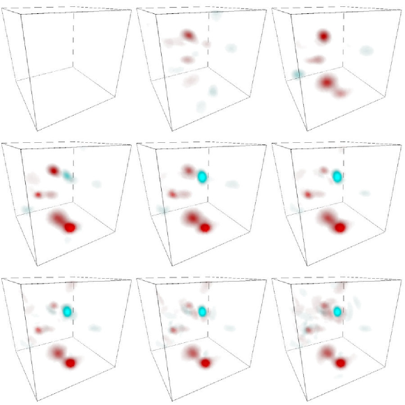
Figure 9: 3D plot of Chern-Simons number density for times $tm_{\rm H}=7$, 8, …, 15. Red: positive, blue: negative.

Figure 8 shows an example of the development of $\langle\varphi^{\dagger}\varphi\rangle$, $\langle N_{\rm CS}\rangle$ and $\langle N_{\rm w}\rangle$. We see Higgs length at first rising exponentially and then executing a damped oscillation around its finite-temperature equilibrium. The CP violation causes an asymmetry in the Chern-Simons number, close to the average winding number, which settles earlier. This leads to a baryon asymmetry $n_{B}/n_{\gamma}\approx(4\pm 1)10^{-5}\,\delta$, which fits observation for the quite reasonable looking value $\delta\approx 1.5\;10^{-5}$.

Example: winding defects [34]

A more detailed understanding of the production of Chern-Simons number might enable us to get more grip on the effects of different forms of CP violation, e.g. by reducing the number of variables through modelling. This production appears to be seeded by regions with winding number of $\approx\pm 1/2$, ‘half-knots’ [34]. Figure 9 shows an example the development of the Chern-Simons number density in the tachyonic electroweak quench. Parameters and initial conditions as in Fig. 7.

Example: kinetic turbulence and scaling [35, 36]

Recently it was demonstrated that concepts of turbulence apply very well to preheating dynamics [35]. Coefficients of power laws and scaling relations were derived on the basis of Boltzmann equations for classical fields, and applied successfully to results of numerical simulations of an inflaton field interacting with itself and with another scalar field [35]. In a contribution to this meeting, similar behavior was shown to apply to a tachyonic electroweak transition [36]. This simulation included the U(1) hypercharge/electromagnetic field, as it was motivated by investigating a seeding mechanism for the currently observed magnetic fields on large scales. Parameters: $m_{W}=6.15$ GeV, $m_{\rm H}/m_{W}=4.65$, $M(t_{\rm i}-t_{c})=5$ (cf. (4)), $g_{SU(2)}/g_{U(1)}$ as in Standard Model.

Figure 10 shows power-law behavior of the variance of the Higgs and inflaton fields, and scaling of the $W$-particle numbers (defined here in terms of the energy spectrum).

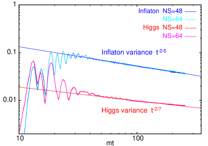
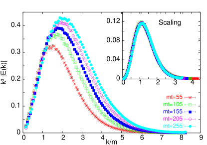
Figure 10: Left: turbulent scaling of Higgs $\langle\varphi\varphi^{\dagger}\rangle$ and inflaton $\langle\sigma\sigma\rangle$ $\propto t^{-\nu}$, $\nu=-2/(2m-1)$, $m=3$ ($\sigma$), $m=4$ (H). Right: self-similar SU(2) spectrum: $n(k,t)=t^{-q}\,n_{0}(kt^{-p})$, $q=(7/2)p$, $p=1.1/7$. From [36].

4 $\Phi$-derivable approximation

At larger times the universe is expected to approach local equilibrium if the dynamics is fast relative to the Hubble rate. Then the classical approximation breaks down because the energy becomes re-distributed over all field modes (equipartition), either leading to lattice artefacts of the Rayleigh-Jeans type, or causing the effective temperature to vanish in case of no cutoff. A quantum description is needed to be able to describe true thermalization through scattering and damping. This has also a non-perturbative features, e.g. a damped oscillation $e^{-\gamma t}\cos(\omega t)$ with $\gamma=c\lambda^{2}$ misses essential features when retaining only low orders of the expansion $e^{-\gamma t}=1-c\lambda^{2}+\cdots$. In diagrammatic language, we need to sum an infinite series of diagrams, in particular for two-point functions. One possibility is using the hierarchy of Dyson-Schwinger equations. Recently so-called $\Phi$-derivable approximations [37, 38] have been used in numerical simulations, and found to be able to capture thermalization [39]. It is a real-time effective-action method in which the two-point function is treated as a basic dynamical variable, in addition to the mean field. The effective action is written as [40]

$$\Gamma(\phi,G)=S(\phi)-\frac{i}{2}\mbox{Tr}\ln G+\frac{i}{2}\mbox{Tr}\frac{\delta^{2}S(\phi)}{\delta\phi\delta\phi}\,G+\Phi(\phi,G),$$

where $S$ is the classical action, $G$ is the two-point function, and $\Phi$ is a sum of two-particle irreducible (2PI) diagrams,

(12)

with bare vertex functions and dressed two-point functions $G$. The equations of motion are given by

$$\frac{\delta\Gamma(\phi,G)}{\delta\phi(x)}=0,\quad\frac{\delta\Gamma(\phi,G)}{\delta G(x,y)}=0,$$

and after separation into contributions with definite time-ordering, indicated by $>$, they have a non-local form, e.g. for $G$:

$$\left[\partial^{2}-\mu^{2}-3\lambda\phi^{2}-3\lambda G(x,x)\right]G^{>}(x,y) = 2\int_{0}^{x^{0}}dz^{0}\int d^{3}z\;{\rm Im}[\Sigma^{>}(x,z;\phi,G)]G^{>}(z,y)$$

$$\mbox{}-2\int_{0}^{y^{0}}dz^{0}\int d^{3}z\;\Sigma^{>}(x,z;\phi,G)\,{\rm Im}[G^{>}(z,y)].$$

Here the selfenergy,

$$\Sigma(x,y)=2i\frac{\delta\Phi}{\delta G(x,y)},$$

is again given by a series of diagrams,

(14)

Interesting aspects of $\Phi$-derivable methods are:
- they are ‘thermodynamically consistent’ [37]
- global symmetries $\to$ Ward-Takahashi Identities,
e.g. translation invariance $\to$ energy-momentum conservation
- they are renormalizable [41, 42, 43, 44, 45, 46, 47, 48]

$\Phi$-derivable approximations are obtained by truncating an expansion of $\Phi$, guided by the number of loops, or the order in a coupling- or $1/N$-expansion [38, 49]. Putting $\Gamma$ on a space-time lattice leads to a numerically viable, albeit computationally expensive scheme. The non-locality of (4) in space can be taken care of (in the usual homogeneous case) by Fourier transformation, which gives an e.o.m. for each Fourier mode. The non-locality in time, while in accordance with causality, leads to numerically expensive ‘memory kernels’. Moreover, these kernels themselves can only be computed in simple approximations, e.g. keeping only diagrams of the type given in the first line in (14); for example, the diagram shown in the second line has two internal vertices, implying two four-dimensional summations over space-time, which is too expensive, numerically.

Initial conditions are given in terms of $\phi$ and $G$, and the results of solving the e.o.m. can be used directly for computing expectation values $\langle O\rangle$ of observables $O(\phi,G)$ – there is no need for averaging over initial configurations as in classical approximations.

Figure 11: Left: Equal-time $F_{V}(t,{\bf p};t,{\bf p})$ vs time for several $p$ and two initial conditions. Right: Approach to the thermal state: $\ln(-1+1/n_{p})$ vs $p$ at various times. From [50].

Example: chiral quark-meson model [50]

The lagrangian of the model is of the Yukawa form

$$-{\cal L}=\bar{\psi}\gamma^{\mu}\partial_{\mu}\psi+\textstyle{\frac{1}{2}}(\partial_{\mu}\sigma\partial^{\mu}\sigma+\partial_{\mu}\pi^{a}\partial^{\mu}\pi^{a})+\textstyle{\frac{1}{2}}\,\mu^{2}(\sigma^{2}+\pi^{a}\pi^{a})+g\bar{\psi}(\sigma+i\gamma_{5}\tau^{a}\pi^{a})\psi,$$

where the $\tau^{a}$ are Pauli matrices, and $\Phi$ is truncated to the simple diagram

(15)

In ref. [50] the two-point functions are split into real and imaginary parts, $G(x,y)\sim F(x,y)-i\rho(x,y)/2$, with spectral functions $\rho$ and ‘statistical functions’ $F$, and the discretization is done directly for the e.o.m. in terms of components of the fermion two-point function, as in

$$\rho=\rho_{S}+\rho_{P}\,i\gamma_{5}+\rho_{V}^{\mu}\gamma_{\mu}+\rho_{A}^{\mu}\gamma_{\mu}\gamma_{5}+\textstyle{\frac{1}{2}}\rho_{T}^{\mu\nu}\sigma_{\mu\nu}.$$

Remarkably, no fermion-doubling was observed.

Figure 11(left) shows spatially Fourier transformed $F_{V}(t,{\bf p};t,{\bf p})$ vs time for three values of $p$ and two different initial conditions. The Yukawa coupling $g=1$. Memory of the initial condition gets lost, which can be phrased in terms of a damping time $1/\gamma_{\rm F}^{\rm damp}\approx 15\,m^{-1}$, with $m$ a ‘thermal mass’. The approach to the final values takes much longer. Figure 11 (right) shows the fermion particle-distribution function $n_{p}$ at various times in the form $\ln(-1+1/n_{p})$, starting from an initial condition out of equilibrium. At large times it approaches the line $p/T$, corresponding to the Fermi-Dirac distribution $n_{p}=1/(1+e^{p/T})$ for a massless fermion. So this is clear evidence for quantum thermalization. Deviations from the FD form due to the interactions appear to be small, even for a Yukawa coupling as large as $g=1$. The approach to the FD form can be analyzed in terms of a thermalization time $1/\gamma_{\rm F}^{\rm therm}\approx 95\,m^{-1}$.

Example: tachyonic ‘electroweak’ quench [51]

In this study the scalar sector of the Standard Model is extended to the $O(N)$ model

$$-{\cal L}=\textstyle{\frac{1}{2}}\,\partial_{\mu}\phi_{\alpha}\partial^{\mu}\phi_{\alpha}-\textstyle{\frac{1}{2}}\,\mu^{2}\phi_{\alpha}\phi_{\alpha}+\frac{1}{4}\,\lambda(\phi_{\alpha}\phi_{\alpha})^{2},\quad\alpha=1,\ldots,N,$$

where $\lambda\propto 1/N$. The functional $\Phi$ is approximated to Next-to-Leading-Order in the $1/N$ expansion [38, 49], after which $N$ is set equal to the SM value 4.

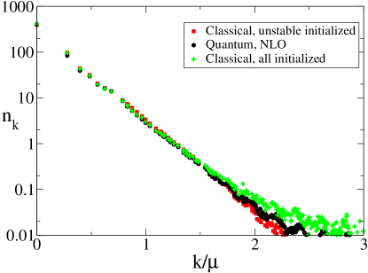
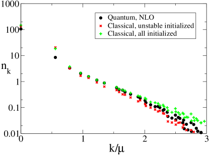
Figure 12: Left: particle numbers at time $t\mu=14$; $\lambda=1/24$ ($m_{\rm H}=71$ GeV), $L\mu=22.4$, $a_{s}\mu=0.7$. Right: similar for stronger coupling $\lambda=1/4$ ($m_{\rm H}=174$ GeV), but smaller volume $L\mu=11.2$. From [51].

Figure 12 shows a comparison with the classical approximation for the same model with $N=4$ (without $1/N$ expansion). The initial conditions correspond to the quench (6), so vacuum initial two-point function $G$ in the quantum $\Phi$-derivable approximation, and ‘just the half’ in the classical approximation, with two choices of $k_{\rm max}$ in (9): $k_{\rm max}=\mu$ (‘unstable initialized’) and ‘cutoff’ (‘all initialized’). It is reassuring that at time $t\mu=14$ the two classical approximations still agree nicely with the $\Phi$-derivable one. (Such confirmation has been found earlier in 1+1 dimensions [52].) This agreement has diminished at time $t\mu=100$, and it reduces further as time progresses, although the general shape of the classical spectra remains similar to the quantal for many hundreds of $t\mu$. Taking the $\Phi$-derivable approximation as a benchmark, the $k_{\rm max}=$ ‘cutoff’ implementation of the classical approximation appears to be somewhat more accurate in these plots.

5 Conclusion and outlook

Before putting a quantum field out of equilibrium on the computer, approximations had to be made. Classical approximations can be well motivated in a limited time regime and they have produced many interesting results. The dominating classical modes have a minimum wavelength, which makes it feasible to include topological observables such as winding and Chern-Simons number densities, and even corresponding terms in the equations of motion, that are notoriously difficult to deal with in the quantum theory. We had no time to go into the question of the size of topological defects in gauge theories [53]. More work is needed on non-abelian gauge fields without Higgs fields, in view of the issues raised in [54].

In the quantum domain $\Phi$-derivable approximations appear to be working well also for late times, and the expected features of quantum thermalization have been observed in scalar and Yukawa models. The implementation of Nambu-Goldstone bosons is still an issue [55, 56, 48, 46]. Gauge theories have to my knowledge not been simulated yet with this method. In case of three-point interactions (generic in gauge theories and also in scalar field models with non-zero mean field), the two-loop selfenergies have contributions that are prohibitively numerically expensive. There is the problem of dependence on the gauge-fixing parameter. It has been argued that such gauge dependence is acceptable as part of the approximation [57]. For non-abelian gauge theory without Higgs fields, the growth of the coupling in the infrared makes it hard to find good truncations.

With fermions there are the usual issues associated with doubling in lattice simulations [58, 59], although this may be avoidable to some extent in non-gauge theories [50]. Perhaps the need to fix the gauge is a blessing in disguise for chiral gauge theories. Real-time simulations with fermions might provide an alternative treatment of finite-density.

Finally, in some cases the Hubble expansion effectively causes the lattice spacing to grow in time, which puts limits on the meaningful duration of the simulation. And here is still lots to do in numerical simulations of the Big Bang.

References

- [1] E. W. Kolb and M. S. Turner, The Early Universe. Addison-Wesley, Reading, Massachusetts, 1990.
- [2] A. R. Liddle and D. H. Lyth, Cosmological inflation and large-scale structure. Cambridge University Press, Cambridge, UK, 2000.
- [3] M. Bastero-Gil and A. Berera, Determining the regimes of cold and warm inflation in the SUSY hybrid model, Phys. Rev. D71 (2005) 063515, [hep-ph/0411144].
- [4] L. Kofman, A. D. Linde, and A. A. Starobinsky, Towards the theory of reheating after inflation, Phys. Rev. D56 (1997) 3258–3295.
- [5] G. N. Felder et al., Dynamics of symmetry breaking and tachyonic preheating, Phys. Rev. Lett. 87 (2001) 011601, [hep-ph/0012142].
- [6] N. Turok, Global texture as the origin of cosmic structure, Phys. Rev. Lett. 63 (1989) 2625.
- [7] M. Broadhead and J. McDonald, Simulations of the end of supersymmetric hybrid inflation and non-topological soliton formation, Phys. Rev. D72 (2005) 043519, [hep-ph/0503081].
- [8] E. Farhi, N. Graham, V. Khemani, R. Markov, and R. Rosales, An oscillon in the SU(2) gauged higgs model, hep-th/0505273.
- [9] M. Dine and A. Kusenko, The origin of the matter-antimatter asymmetry, hep-ph/0303065.
- [10] W. Buchmuller, R. D. Peccei, and T. Yanagida, Leptogenesis as the origin of matter, hep-ph/0502169.
- [11] J. García-Bellido, D. Y. Grigoriev, A. Kusenko, and M. E. Shaposhnikov, Non-equilibrium electroweak baryogenesis from preheating after inflation, Phys. Rev. D60 (1999) 123504, [hep-ph/9902449].
- [12] L. M. Krauss and M. Trodden, Baryogenesis below the electroweak scale, Phys. Rev. Lett. 83 (1999) 1502–1505, [hep-ph/9902420].
- [13] E. J. Copeland, D. Lyth, A. Rajantie, and M. Trodden, Hybrid inflation and baryogenesis at the TeV scale, Phys. Rev. D64 (2001) 043506, [hep-ph/0103231].
- [14] J. García-Bellido, M. García-Pérez, and A. González-Arroyo, Chern-Simons production during preheating in hybrid inflation models, Phys. Rev. D69 (2004) 023504, [hep-ph/0304285].
- [15] A. Tranberg and J. Smit, Baryon asymmetry from electroweak tachyonic preheating, JHEP 11 (2003) 016, [hep-ph/0310342].
- [16] S. Hannestad, What is the lowest possible reheating temperature?, Phys. Rev. D70 (2004) 043506, [astro-ph/0403291].
- [17] G. Aarts and J. Smit, Finiteness of hot classical scalar field theory and the plasmon damping rate, Phys. Lett. B393 (1997) 395–402, [http://arXiv.org/abs/hep-ph/9610415].
- [18] G. Aarts and J. Smit, Classical approximation for time-dependent quantum field theory: Diagrammatic analysis for hot scalar fields, Nucl. Phys. B511 (1998) 451–478.
- [19] M. Sallé, J. Smit, and J. C. Vink, Thermalization in a Hartree ensemble approximation to quantum field dynamics, Phys. Rev. D64 (2001) 025016.
- [20] S. Mrowczynski and B. Muller, Wigner functional approach to quantum field dynamics, Phys. Rev. D50 (1994) 7542–7552, [hep-th/9405036].
- [21] T. Asaka, W. Buchmuller, and L. Covi, False vacuum decay after inflation, Phys. Lett. B510 (2001) 271–276, [hep-ph/0104037].
- [22] J. García-Bellido, M. García-Pérez, and A. González-Arroyo, Symmetry breaking and false vacuum decay after hybrid inflation, Phys. Rev. D67 (2003) 103501, [hep-ph/0208228].
- [23] J. Smit and A. Tranberg, Chern-Simons number asymmetry from CP violation at electroweak tachyonic preheating, JHEP 12 (2002) 020, [hep-ph/0211243].
- [24] T. Yavin, Classical simulation of quantum , These proceedings.
- [25] J. Ambjorn, T. Askgaard, H. Porter, and M. E. Shaposhnikov, Sphaleron transitions and baryon asymmetry: A numerical real time analysis, Nucl. Phys. B353 (1991) 346–378.
- [26] J. Ambjorn and A. Krasnitz, The classical sphaleron transition rate exists and is equal to , Phys. Lett. B362 (1995) 97–104.
- [27] D. Bodeker, G. D. Moore, and K. Rummukainen, Chern-Simons number diffusion and hard thermal loops on the lattice, Phys. Rev. D61 (2000) 056003, [hep-ph/9907545].
- [28] S. Y. Khlebnikov and I. I. Tkachev, Classical decay of inflaton, Phys. Rev. Lett. 77 (1996) 219–222, [hep-ph/9603378].
- [29] M. Desroche, G. N. Felder, J. M. Kratochvil, and A. Linde, Preheating in new inflation, Phys. Rev. D71 (2005) 103516, [hep-th/0501080].
- [30] S. Borsanyi, A. Patkos, and D. Sexty, Non-equilibrium goldstone phenomenon in tachyonic preheating, Phys. Rev. D68 (2003) 063512, [hep-ph/0303147].
- [31] E. J. Copeland, S. Pascoli, and A. Rajantie, Dynamics of tachyonic preheating after hybrid inflation, Phys. Rev. D65 (2002) 103517, [hep-ph/0202031].
- [32] J.-I. Skullerud, J. Smit, and A. Tranberg, W and Higgs particle distributions during electroweak tachyonic preheating, JHEP 08 (2003) 045, [hep-ph/0307094].
- [33] A. Tranberg, Simulations of cold electroweak baryogenesis, These proceedings.
- [34] D. Sexty, J. Smit, A. Tranberg, and M. van der Meulen, Chern-Simons and winding number in a tachyonic electroweak transition, In preparation.
- [35] R. Micha and I. I. Tkachev, Turbulent thermalization, Phys. Rev. D70 (2004) 043538, [hep-ph/0403101].
- [36] A. Diaz-Gil, J. Garcia-Bellido, M. G. Perez, and A. Gonzalez-Arroyo, Magnetic field production after inflation, hep-lat/0509094.
- [37] G. Baym, Selfconsistent approximation in many body systems, Phys. Rev. 127 (1962) 1391–1401.
- [38] J. Berges, Nonequilibrium quantum fields and the classical field theory limit, Nucl. Phys. A702 (2002) 351–355, [hep-ph/0201204].
- [39] J. Berges and J. Cox, Thermalization of quantum fields from time-reversal invariant evolution equations, Phys. Lett. B517 (2001) 369–374, [hep-ph/0006160].
- [40] J. M. Cornwall, R. Jackiw, and E. Tomboulis, Effective action for composite operators, Phys. Rev. D10 (1974) 2428–2445.
- [41] H. van Hees and J. Knoll, Renormalization in self-consistent approximations schemes at finite temperature. I: Theory, Phys. Rev. D65 (2002) 025010.
- [42] H. Van Hees and J. Knoll, Renormalization of self-consistent approximation schemes. II: Applications to the sunset diagram, Phys. Rev. D65 (2002) 105005.
- [43] J.-P. Blaizot, E. Iancu, and U. Reinosa, Renormalizability of -derivable approximations in scalar theory, Phys. Lett. B568 (2003) 160–166.
- [44] J.-P. Blaizot, E. Iancu, and U. Reinosa, Renormalization of -derivable approximations in scalar field theories, Nucl. Phys. A736 (2004) 149–200.
- [45] F. Cooper, B. Mihaila, and J. F. Dawson, Renormalizing the Schwinger-Dyson equations in the auxiliary field formulation of field theory, Phys. Rev. D70 (2004) 105008, [hep-ph/0407119].
- [46] F. Cooper, J. F. Dawson, and B. Mihaila, Renormalized broken-symmetry Schwinger-Dyson equations and the 2PI-1/N expansion for the O(N) model, Phys. Rev. D71 (2005) 096003, [hep-ph/0502040].
- [47] J. Berges, S. Borsanyi, U. Reinosa, and J. Serreau, Renormalized thermodynamics from the 2PI effective action, Phys. Rev. D71 (2005) 105004, [hep-ph/0409123].
- [48] J. Berges, S. Borsanyi, U. Reinosa, and J. Serreau, Nonperturbative renormalization for 2PI effective action techniques, hep-ph/0503240.
- [49] G. Aarts, D. Ahrensmeier, R. Baier, J. Berges, and J. Serreau, Far-from-equilibrium dynamics with broken symmetries from the 2PI-1/N expansion, Phys. Rev. D66 (2002) 045008, [hep-ph/0201308].
- [50] J. Berges, S. Borsanyi, and J. Serreau, Thermalization of fermionic quantum fields, Nucl. Phys. B660 (2003) 51–80.
- [51] A. Arrizabalaga, J. Smit, and A. Tranberg, Tachyonic preheating using 2PI-1/N dynamics and the classical approximation, JHEP 10 (2004) 017, [hep-ph/0409177].
- [52] G. Aarts and J. Berges, Classical aspects of quantum fields far from equilibrium, Phys. Rev. Lett. 88 (2002) 041603, [hep-ph/0107129].
- [53] M. Hindmarsh and A. Rajantie, Defect formation and local gauge invariance, Phys. Rev. Lett. 85 (2000) 4660–4663, [cond-mat/0007361].
- [54] G. D. Moore, Problems with lattice methods for electroweak preheating, JHEP 11 (2001) 021, [hep-ph/0109206].
- [55] H. van Hees and J. Knoll, Renormalization in self-consistent approximation schemes at finite temperature. III: Global symmetries, Phys. Rev. D66 (2002) 025028.
- [56] Y. B. Ivanov, F. Riek, H. van Hees, and J. Knoll, Renormalized phi-derivable approximations to theory with spontaneously broken O(N) symmetry, hep-ph/0506157.
- [57] A. Arrizabalaga and J. Smit, Gauge-fixing dependence of -derivable approximations, Phys. Rev. D66 (2002) 065014.
- [58] G. Aarts and J. Smit, Real-time dynamics with fermions on a lattice, Nucl. Phys. B555 (1999) 355–394, [http://arXiv.org/abs/hep-ph/9812413].
- [59] G. Aarts and J. Smit, Particle production and effective thermalization in inhomogeneous mean field theory, Phys. Rev. D61 (2000) 025002, [hep-ph/9906538].