Transport Coefficients of Gluon Plasma from Lattice QCD

Abstract:

RHIC is now confirming the discovery of the “New State of Matter”, whose properties are gradually revealed by experimental data. It is not the free gas state, but well described by a fluid with very small viscosity. It is now highly desired to calculate the value of the viscosity from the fundamental theory, i.e., QCD just above the transition temperature. In this report we present our calculation of the transport coefficient of gluon system on $24^{3}\times 8$ lattice in the quench approximation. Simulations are carried out in the range, $1.4\leq T/T_{c}\leq 24$. In the temperature region slightly above the transition, where the perturbative calculation is not applicable, the shear viscosity($\eta$) is smaller than typical hadron masses. The bulk viscosity is consistent with zero within the range of error bars in $1.4\leq T/T_{c}\leq 24$. We compare our results with the perturbative calculations in large $T/T_{c}$ region. It is found that the lattice and perturbative results are consistent with each other there. The ratio $\eta/s$ is around $0.1-0.4$ in $T/T_{c}<3$ region and satisfies the KSS bound[14]. In order to estimate the contribution from high frequency part of the spectral function, we study the effects of a term $\rho^{high}$ proposed by Aarts and Resco[3]. It is found that until the threshold mass becomes small, its effect is quite small, and that viscosity decreases as the threshold decreases. From these studies we think that although our result is obtained under an assumptions for the spectral function, it gives a reasonable estimation for $\eta$($=\pi d\rho/d\omega$ at $\omega=0$), and qualitative results will not be changed when the accurate spectral function is obtained.

PoS(LAT2005)186

1 Introduction

The RHIC data are now revealing some properties of a “New State of Matter”, which is expected to be quark-gluon plasma(QGP). The jet quenching data suggest that its mean free path is short, and the phenomenological analysis of the elliptic flow shows that, it could be explained by a fluid model with small viscosity. Namely it is almost perfect fluid. As the viscosity is proportional to mean free path[1], this analysis also indicates that mean free path is short. The mean free path $\lambda$ is related to scattering cross section $\sigma$ and the number density $n$ as $\lambda\propto 1/(\sigma n)$. Therefore the small $\lambda$, means that the “New State of Matter” is a strongly interacting system.

It is a natural anticipation that transport coefficients of the QGP must be smaller than an ordinary matter, like water or oil etc., because QCD coupling in the deconfined phase will be larger than the electromagnetic coupling constant $1/137$, but its value must be calculated from fundamental theory of QCD. Therefore it is now urgent to calculate transport coefficients by fully taking into account non-perturbative effects, because QGP near the transition temperature will be strongly interacting In Ref.[2] we published our results from lattice simulations in the $1.5<T/T_{c}<2.1$ region. In this report, the study is extended to higher temperature region, $T/T_{c}<24$, and we compare our results with perturbative calculations there. We also discuss how our results depend on the spectral function of the green function in high frequency region[3].

On a lattice, calculation of the transport coefficients is formulated in the framework of the linear response theory[4, 5].

$$\eta=-\int d^{3}x^{\prime}\int_{-\infty}^{t}dt_{1}e^{\epsilon(t_{1}-t)}\int_{-\infty}^{t_{1}}dt^{\prime}<T_{12}(\vec{x},t)T_{12}(\vec{x^{\prime}},t^{\prime})>_{ret}$$ (1)

$$\frac{4}{3}\eta+\zeta=-\int d^{3}x^{\prime}\int_{-\infty}^{t}dt_{1}e^{\epsilon(t_{1}-t)}\int_{-\infty}^{t_{1}}dt^{\prime}<T_{11}(\vec{x},t)T_{11}(\vec{x^{\prime}},t^{\prime})>_{ret}$$ (2)

where $\eta$ is shear viscosity, and $\zeta$, bulk viscosity. $<T_{\mu\nu}T_{\rho\sigma}>_{ret}$ is a retarded Green’s function of energy momentum tensor at a given temperature. In the quenched model, $T_{\mu\nu}$ is written by the field strength tensor as follows.

$$T_{\mu\nu}=2Tr[F_{\mu\sigma}F_{\nu\sigma}-\frac{1}{4}\delta_{\mu\nu}F_{\rho\sigma}F_{\rho\sigma}]$$ (3)

The field strength tensor is defined by the plaquette operator, $U_{{}\mu\nu}(x)=\exp{(ia^{2}gF_{\mu\nu}(x))}$.

The shear viscosity in Eq.1 is also expressed by using a spectral function $\rho$ of the retarded Green’s function $\rho(\omega)$[5] as follows.

$$\eta=\pi\displaystyle{\lim_{\omega\rightarrow 0}}\frac{\rho(\omega)}{\omega}=\pi\lim_{\omega\rightarrow 0}\frac{d\rho(\omega)}{d\omega}$$ (4)

For the determination of the spectral function $\rho(\omega)$, we use a well known fact that the spectral function of the retarded Green’s function at temperature $T$ is same as that of Matsubara-Green’s function. Therefore our target is to calculate Matsubara-Green’s function($G_{\beta}(t_{n})$) on a lattice and determine $\rho(\omega)$ from it.

2 Lattice calculation of $\eta$ from Matsubara-Green’s function $G_{\beta}(t)$

Using the spectral function $\rho(\omega)$, $G_{\beta}(t)$ is expressed as follows

$$G_{\beta}(t)=-\frac{1}{\beta}\sum_{n}e^{-iw_{n}t}\int_{-\infty}^{\infty}\frac{\rho(\omega)}{i\omega_{n}-\omega}d\omega=\int_{0}^{\infty}\frac{cosh(\omega(t-\beta/2))}{sinh(\omega\beta/2)}\rho(\omega)d\omega,$$ (5)

where $\omega_{n}=2\pi n/\beta$. Note that the last equality holds for the region $0<t<\beta(N_{T})$: at $t=0$ and $\beta(=N_{T})$ it could not be used.

In order to determine the spectral function $\rho(\omega)$ from $G_{\beta}(t_{n})$, which is given at discrete points $t_{n}=1,2...,N_{T}-1$ on a lattice, the most promising method may be the maximum entropy method(MEM). However to determine the $\rho(\omega)$ precisely by MEM, $G_{\beta}(t_{n})$ on $N_{T}>30$ lattice with high statistics is necessary. However, we realized that $G_{\beta}(t_{n})$ is very noisy[6], and we decided to start with a relatively smaller lattice of large statistics with some assumption for the spectral function $\rho(\omega)$.

The simplest non trivial form is a Bright-Wigner type proposed by Karsch and Wyld[7].

$$\rho_{BW}(\omega)=\frac{A}{\pi}(\frac{\gamma}{(m-\omega)^{2}+\gamma^{2}}-\frac{\gamma}{(m+\omega)^{2}+\gamma^{2}}).$$ (6)

In this case, shear viscosity is given by $\eta=4A\gamma m/(\gamma^{2}+m^{2})^{2}$, similarly for bulk viscosity $\zeta$. As this formula already has 3 parameters, in order to determine them by least squares, the lattice size in temperature direction($N_{T}$) must be $N_{T}\geq 8$. Then the minimum lattice size is $24^{3}\times 8$, to obtain a non trivial results.

Simulations are carried out by using the Iwasaki’s improved action and standard Wilson action. The simulation points are at $\beta=$3.05, 3.3, 4.5 and 5.5 for the improved action and $\beta$=7.5 and 8.5 for Wilson action. With roughly $10^{6}$ MC measurements at each $\beta$, we determine the Matsubara-Green’s functions $G_{\beta}(t_{n})$ as shown in Fig. 1.

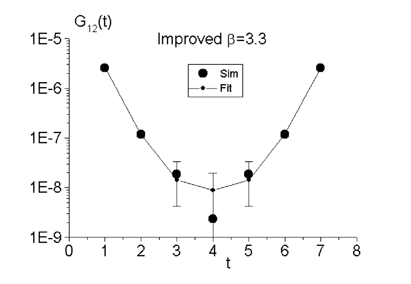
Figure 1: Matsubara-Green’s function $G_{12}(t)$ at $\beta=3.3$

Although the errors of the Matsubara-Green’s function are still not small in large $t$ region, we can fit them with the spectral function $\rho$, given by Eq.6, using a least square package SALS. The fitting range is $1\leq t\leq 4$. The viscosities are calculated from these parameters, and the errors are estimated by the jackknife method. The bin size of the jackknife analysis is taken to be $10^{5}$ and $2\times 10^{5}$ for the improved and Wilson actions, respectively.

The bulk viscosity is equal to zero within the range of error bars, while the shear viscosity remains finite. In order to determine the shear viscosity in physical unit, the lattice spacing $a(\beta)$ must be determined, because, in the lattice calculation, $\eta\times a^{3}$ is obtained. The relation between lattice spacing $a$ and $\beta$ is studied phenomenologically in $2.2\leq\beta\leq 3.8$, and $5.58\leq\beta\leq 6.5$ regions for improved[8] and Wilson actions[9], respectively. In the larger $\beta$ region, we adopt 2-loop renormalization group relation,

$$a(\beta)=\frac{1}{\Lambda}(\frac{6b_{0}}{\beta})^{-\frac{b_{1}}{2b_{0}^{2}}}\exp(\frac{-\beta}{12b_{0}}),$$ (7)

with $b_{0}=33/(48\pi^{2})$, and $b_{1}=(34/3)(3/16\pi^{2})^{2}$. The $\Lambda$ is determined by the $a(\beta)$ at $\beta=$3.8 and 6.5, and they result in $T_{c}/\Lambda=$ 1.26 and 47.35 for the improved and Wilson actions, respectively, where $T_{c}=270$MeV in the quenched model. The results for the shear viscosity are shown in Fig. 2 with circle. It is seen that $\eta$ from both actions are consistent with each other.

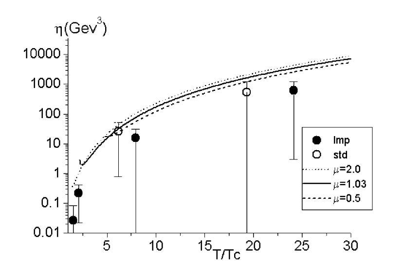
Figure 2: Shear viscosity in physical unit from lattice(circles) and perturbative calculations(lines). The lines show the ambiguity due to the choice of the scale parameter in two-loop running coupling formula.

3 Comparison with perturbative results

As we have calculated $\eta$ at rather high temperature region, we compare our results with the perturbative results. The perturbative results are summarized as follows. The bulk viscosity $\zeta$ is zero [5, 10]. The shear viscosity in the next-to-leading log is given by[11],

$$\eta=\frac{\eta_{1}\cdot T^{3}}{g^{4}(\ln(\mu^{*}/gT)},$$ (8)

where $\eta_{1}=27.126$ and $\mu^{*}/T=2.765$, and $g$ is the running coupling constant. We use 2-loop formula for it,

$$g^{-2}(T)=2b_{0}\ln(\mu\frac{T}{T_{c}})+\frac{b_{1}}{b_{0}}\ln\left(2\ln(\mu\frac{T}{T_{c}})\right)$$ (9)

Note that the perturbative approximations are renormalization-scale $\mu$ dependent. The simplest choice would be $\mu=T_{c}/\Lambda_{QCD}\sim 1.03$[12]. However in order to see the ambiguity of the perturbative result due to $\mu$, we change $\mu$ in the range $0.5\leq\mu\leq 2$. The results are also shown in Fig. 2 with line. In the large $T$ region, the $\mu$ dependence is not large. However at smallest $T$ of each line, it shows a small increase. It means the break down of the perturbative calculation. However until the break down starts the agreement of the perturbative and lattice results are satisfactory. From this, we think that although our result depends on the assumption of the $\rho_{BW}$ given in Eq. 6, it may be a reasonable approximation for $d\rho/d\omega$ at $\omega=0$.

Let us proceed to the study of the $\eta/s$ ratio, recently discussed in [13, 14]. The entropy on the lattice is reported by [8] and [15] in $T/T_{c}<4.5$, for improved and Wilson actions respectively. In the higher temperature region, where the data are not available, we use the high temperature limit values on $N_{T}=8$ lattice. The results are shown in Fig. 3 with circles. For the perturbative result on entropy, we use the formula of hard thermal loop calculation up to order $g^{3}$[12]. The results are also shown in Fig.3 with lines.
As explained in the Fig.2, the slight increase at the small $T$ region is observed for the perturbative results, indicating breakdown of perturbative calculations. The agreement between these two calculations are not good enough. However we do not think that it is a real difficulty. Because if we decrease the scale parameter $\mu$, the agreement is improved. An important information from these results is the qualitative magnitude of the ratio $\eta/s$. In the $T/Tc<3$ region, the ratio is small (0.1-0.4), where the perturbative results diverges. And for all the temperature regions we have studied, it is less than one. We don’t think that it would become 10 times of present value, when the accurate determination of the spectral function is carried out.

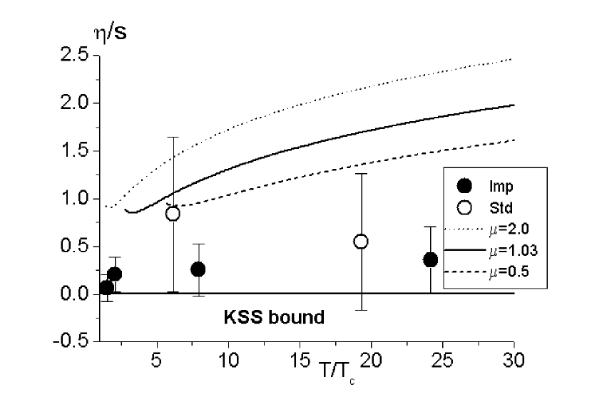
Figure 3: $\eta/s$ obtained by lattice simulations(circles) and perturbative calculations(lines). The $\mu$ is a scale parameter in the running coupling constant of Eq.3.2

4 Discussions and conclusions

4.1 Fit of $G_{\beta}$ by other spectral functions

Aarts and Resco have proposed an another form for the spectral function $\rho$[3],

$$\rho(\omega)=\rho^{low}(\omega)+\rho^{high}(\omega)$$ (10)

$$\frac{\rho^{low}(\omega)}{T^{4}}=x\frac{b_{1}+b_{2}x^{2}+...}{1+c_{1}x^{2}+c_{2}x^{4}+..},\hskip 28.45274ptx=\frac{\omega}{T}$$ (11)

$$\rho^{high}(\omega)=\theta(\omega-2m_{th})\frac{d_{A}(\omega^{2}-4m_{th}^{2})^{5/2}}{80\pi^{2}\omega}[n(\omega/2)+0.5]$$ (12)

where $d_{A}=N_{c}^{2}-1$, and $n(\omega)=1/(\exp(\omega/T)-1)$. We consider three parameters case, $b_{1}$, $c_{1}$ and $m_{th}$. The fit by SALS could be made but $c_{1}<0$.

We would like to remember that the spectral function $\rho$ must satisfy the sum rule[16],

$$\int_{-\infty}^{\infty}\frac{1}{2\pi}\omega\rho(\omega)d\omega=1.$$ (13)

In the full parameter representation, the cancellation of the divergence between $\rho^{low}$ and $\rho^{high}$ in high $\omega$ region results in the convergence of the integration. But in this three parameter form, the $\rho$ could not satisfy the sum rule. Then some modification is necessary. But in this work we applied the unmodified form. Because the integration over $\omega$ in Eq.5 converges due to the term $cosh(\omega(t-\beta/2))/sinh(\omega\beta/2)$, except for $t=0$ and $t=\beta$, we think that phenomenologically, a possible contribution from high frequency part of $\rho(\omega)$ could be studied in this form.

As the another trial, we study effects of $\rho^{high}$ for the shear viscosity $\eta$. We assume $\rho$ is given by $\rho=\rho_{BW}+\rho^{high}$, where $\rho_{BW}$ is given by Eq. 6. By changing $m_{th}$, the change of $\eta$ is studied at $\beta=3.3$ for the improved action. When $\rho^{high}$ is absent ($m_{th}=\infty$), $\eta a^{3}$=0.00225(201). If $m_{th}$ is set to be 5.0, 3.0 and 2.0, $\eta a^{3}$ becomes 0.00223(0.00191), 0.00194(0.00194) and 0.00126(0.00204), respectively. And at $m_{th}=1.8$, the contribution from $\rho^{high}$ becomes larger than the $G_{\beta}(t_{n})$ of simulation at $t=1$, that fit could not be done. Generally as $m_{th}$ decreases the contribution from $\rho^{high}$ increases and the $\rho$ in the small $\omega$ region is suppressed. In this case, it results in the decrease of $\eta$.

In this case, the $\rho_{BW}$ (without $\rho^{high}$), determined by SALS to fit the Matsubara Green’s function, satisfies the relation,

$$\int_{-\infty}^{\infty}\frac{1}{2\pi}\omega\rho_{BW}(\omega)d\omega<1.$$ (14)

As a full spectral function $\rho$ will have contributions from scattering states etc., in addition to Bright-Wigner type, Eq.14 does not mean that the full spectral function violates the sum rule.

4.2 Conclusion and further studies

On $24^{3}\times 8$ lattice, we have calculated the Matsubara-Green’s function and determine the transport coefficients of gluon plasma. The bulk viscosity is consistent with zero, while shear viscosity remains finite, within the error bars of present statistics. In the high temperature region, the agreement of the lattice and perturbative calculation is satisfactory for the shear viscosity. The lattice result on ratio $\eta/s$ in $T/T_{c}\leq 3$ is smaller than the extrapolation of the perturbative calculation and satisfies the KSS bound.

Although our results depend on the form of the spectral function $\rho_{BW}$ given by Eq.6, we think that the qualitative features will not be changed. Because as discussed in the previous subsection, our results are stable if the high frequency part of the spectral function $\rho^{high}$ is included. It is expected that as $\rho(\omega)$ decreases faster than $\omega^{-2}$ and due to the factor , $cosh(\omega(t-\beta/2))/sinh(\omega\beta/2)$ in Eq.5, the Matsubara Green’s function $G_{\beta}(t)$ will not be sensitive to the behavior of $\rho(\omega)$ in high $\omega$ region, except at $t=0$ and $t=\beta$. We think that the $\eta$ and $\eta/s$ will not become 10 times of the present value when more accurate determination of the transport coefficients are carried out.

However it is important to make a more accurate calculation of the transport coefficients, independent of the assumption of the spectral function. For that goal, we are starting the calculation of $G_{\beta}(t_{n})$ on an anisotropic lattice, to apply the maximum entropy method.

References

- [1] A. Hosoya, M. Sakagami and M. Takao, Nonequilibrium Thermodynamics in Field Theory: Transport Coefficients Annals of Phys. 154, 229(1984)
- [2] A. Nakamura and S. Sakai, Transport Coefficients of Gluon Plasma Phys. Rev. Letters 94,072305(2005)
- [3] G. Aarts and J.M.M. Resco, Transport Coefficients: spectral function and the lattice JHEP 4, 53(2002)
- [4] D.N. Zubarev, Non-equilibrium statistical mechanics, Plenum, New York, 1974
- [5] R. Horsley, W. Schoenmaker, Quantum Field Theories out of Thermal Equilibrium, (I).General considerations, (II). The transport coefficients for QCD Nucl. Phys. B280[FS18],716,735(1987)
- [6] A. Nakamura, T. Saito and S. Sakai, Numerical Results for Transport Coefficients of Quark Gluon Plasma with Iwasaki’s Improved Action Nucl. Phys. B (Proc. Suppl.) 63A-C,424(1998)
- [7] F. Karsch and H.W. Wyld, Thermal Green’s function and transport coefficients on the lattice Phys. Rev. D35, 2518(1987)
- [8] M. Okamoto et al., Equation of state for pure SU(3) gauge theory with renormalization group improved action Phys. Rev.D60, 094510(1999).
- [9] R.G. Edwards. U.M. Heller and T.R. Klassen, Accurate scale determination for the Wilson gauge action Nucl. Phys.B517, 377(1998).
- [10] A. Hosoya and K. Kajantie, Transport Coefficients of QCD Matter Nucl. Phys B250, 666(1985)
- [11] P. Arnold, G.D. Moore and L.G. Yaffe, Transport coefficients in high temperature gauge theories: (II) Beyond leading log l JHEP05 051(2003),[hep-ph/0302165]
- [12] J-P. Blaizot, E. Iancu and A. Rebhan, Entropy of QCD Plasma Phys. Rev. Letters83 2906(1999)
- [13] G. Policastro, D.T. Son and A.O. Starinet, Shear viscosity of strongly coupled N=4 supersymmetric Yang-Mills plasma Phys. Rev. Letters87 081601(2001), [hep-th/0104066]
- [14] P.K. Kovtun, D.T. Son and A.O.Starinets, Viscosity in strongly interacting quantum field theories from black hole physics [hep-th/0405231]
- [15] G. Boyd et a., Thermodynamics of SU(3) lattice gauge theory Nucl.PhysB469 419(1996),[hep-lat/9602007]
- [16] for example, M. Le Bellac Thermal Field Theory p.26, Cambridge University Press,(1996)