Vortex Proliferation and the Dual Superconductor Scenario for Confinement:
The 3D Compact U(1) Lattice Higgs Model

Abstract:

It is argued that the phase diagram of the 3D Compact U(1) Lattice Higgs Model is more refined than generally thought. The confined and Higgs phases are separated by a well-defined phase boundary, marked by proliferating vortices. It is shown that the confinement mechanism at work is precisely the dual superconductor scenario.

PoS(LAT2005)248

1 Introduction

Since a confining state is a very special state of matter, it would be desirable for it to be clearly distinguishable from any other state the system can assume. Ideally, the confining state would be separated from the other states by a phase transition with an order parameter signaling the fundamental change of the ground state. However, by studying the three-dimensional (3D) Abelian Higgs model with compact gauge field, Fradkin and Shenker [1] provided a counterexample. For a Higgs field carrying one unit charge $q=1$, they showed that in the London limit, where the amplitude of the Higgs field is kept fixed, it is always possible to move from the Higgs region into the confined region without encountering singularities in local gauge-invariant observables. As for the liquid-vapor transition, this is commonly interpreted as implying that the two ground states do not constitute distinct phases. This can be further supported by symmetry considerations [2]. The relevant global symmetry for the model with a Higgs field carrying charge $q$ is the cyclic group Z_q of $q$ elements. For $q=2$, this implies the possibility that the confined and Higgs phases are separated by a continuous phase transition belonging to the 3D Ising universality class. This is indeed known to be the case [1, 3]. For $q=1$ on the other hand, this simply excludes a continuous phase transition as the group $Z_{1}$, consisting of only the unit element, cannot be spontaneously broken. We are thus left with the rather unsatisfying situation of having a confined state which is not at all that special, being analytically connected to a different ground state with different, unrelated physical properties, viz the Higgs phase. To address this issue, we numerically investigate the $q=1$ model with fluctuating Higgs amplitude. Similar studies were already carried out as early as in 1985 [4, 5] on smaller lattices, and more recently in Refs. [6, 7] on larger ones. A first report on our findings recently appeared in Ref. [8].

2 Monte Carlo Simulations

The compact Abelian lattice Higgs model is defined by the 3D Euclidean lattice action $S=S_{g}+S_{\phi}$. The gauge part is the standard action for a compact Abelian gauge field

$$S_{g}=\beta\sum_{x,\mu<\nu}\left[1-\cos\theta_{\mu\nu}(x)\right],$$ (1)

where $\beta$ is the inverse gauge coupling. The sum extends over all lattice sites $x$ and lattice directions $\mu$, and $\theta_{\mu\nu}(x)$ denotes the plaquette variable $\theta_{\mu\nu}(x)=\Delta_{\mu}\theta_{\nu}(x)-\Delta_{\nu}\theta_{\mu}(x)$, with the lattice derivative $\Delta_{\nu}\theta_{\mu}(x)\equiv\theta_{\mu}(x+\nu)-\theta_{\mu}(x)$ and the compact link variable $\theta_{\mu}(x)\in[-\pi,\pi)$. The matter part of the action consists of a $|\phi|^{4}$ theory minimally coupled to the gauge field

$$S_{\phi}\!\!=\!\!-\kappa\sum_{x,\mu}\rho(x)\rho(x+\mu)\cos\left[\Delta_{\mu}\varphi(x)-\theta_{\mu}(x)\right]+\sum_{x}\left\{\rho^{2}(x)+\lambda\left[\rho^{2}(x)-1\right]^{2}\right\},$$ (2)

where the complex Higgs field is represented by its amplitude and phase $\phi(x)=\rho(x)\mathrm{e}^{\mathrm{i}\varphi(x)}$, with $\varphi(x)\in[-\pi,\pi)$. The parameter $\kappa$ is the hopping parameter and $\lambda$ the Higgs self-coupling, which together with the inverse coupling constant $\beta$ constitute the parameters of the theory. The model is put on a cubic lattice of linear size $L$ with periodic boundary conditions. The pure $|\phi|^{4}$ theory with fluctuating amplitude, obtained by taking the gauge coupling to zero, i.e., by letting $\beta\to\infty$, was recently investigated by means of Monte Carlo simulations in Ref. [9].

We monitor observables that probe the gauge and matter parts separately. For the gauge part we consider the monopole density $M$ [10] and the Polyakov loop, as was done earlier in Ref. [11], where the London limit of the model was considered. For the matter part we consider the Higgs amplitude squared $\rho^{2}\equiv(1/L^{3})\sum_{x}\rho^{2}(x)$. In addition, we monitor the plaquette action (1) (divided by $3L^{3}$) and the link observable $C=-(1/3L^{3})\sum_{x,\mu}\cos\left[\Delta_{\mu}\varphi(x)-q\theta_{\mu}(x)\right]$. Both Metropolis and heat-bath methods are used to generate Monte Carlo updates. Since these local updates become inefficient at first-order phase transitions, we implement the multicanonical method [12] and reweighting techniques [13] to access these regions of phase space. The simulations are carried out at fixed inverse gauge coupling $\beta$ on cubic lattices varying in size from $6^{3}$ to $32^{3}$, in extreme cases to $42^{3}$. Thermalization of production runs typically take $4\times 10^{4}$ sweeps of the lattice, while about $10^{6}$ sweeps are used to collect data, with measurements taken after each sweep of the lattice. Because of its pronounced peaks, we use the maxima of the link susceptibility $\chi_{C}=L^{3}\left(\langle C^{2}\rangle-\langle C\rangle^{2}\right)$ together with histograms, rescaled to equal height, to trace out the phase boundary. Statistical errors are estimated by means of jackknife binning. For a detailed description of the algorithms and their implementation, the reader is referred to Ref. [14].

3 Phase Diagram

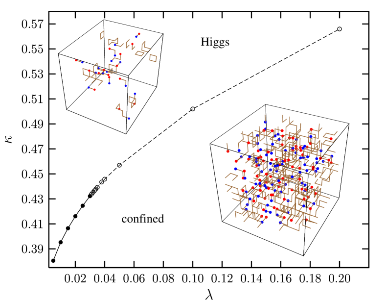
Figure 1: $\kappa$-$\lambda$ phase diagram at $\beta=1.1$ in the infinite-volume limit. Solid dots mark the first-order phase transition line ending at $0.030<\lambda_{\mathrm{c}}<0.032$. Open dots for $\lambda>\lambda_{c}$ mark the location of the Kertész line approaching $\kappa=0.717(2)$ in the London limit $\lambda\to\infty$. The insets show snapshots of typical monopole and vortex configurations in both phases, with red dots denoting monopoles and blue dots denoting antimonopoles, each monopole-antimonopole pair being connected by a vortex.

Figure 1 summarizes our results for $\beta=1.1$. We identify two phases: a confined and a Higgs phase which below a critical point $\lambda_{\mathrm{c}}(\beta)$ are separated by a first-order phase transition as was already observed in the earlier Monte Carlo simulations on smaller lattices [4, 5]. For $\beta=1.1$ we estimate the critical point, where the first-order line ends, to be located in the interval $0.030<\lambda_{\mathrm{c}}(1.1)<0.032$ in the infinite volume limit. The behavior of the average $\langle\rho^{2}\rangle$ identifies the phase in the upper left part of the phase diagram as Higgs phase, where it increases more or less linearly with increasing $\kappa$, while it takes on a minimum value in the confined phase. The average plaquette action takes on a finite value in the confined phase practically independent of $\kappa$ and $\lambda$, while it decreases with increasing $\kappa$ in the Higgs phase. The identification of the two phases is consistent with the behavior of the Polyakov loop we observed.

Of more importance from the perspective of understanding the mechanism leading to charge confinement is the behavior of the monopole density. Monopoles and vortices appear due to compactness of the phase angles $\theta_{\mu}(x)$ and $\varphi(x)$, respectively. Using the compact notations of differential forms on the lattice [15] the monopole charge and vortex current are defined as follows

$$m=\frac{1}{2\pi}\mathrm{d}{[\mathrm{d}\theta]}_{2\pi}\,,\quad j=\frac{1}{2\pi}\left(\mathrm{d}{[\mathrm{d}\varphi-\theta]}_{2\pi}+{[\mathrm{d}\theta]}_{2\pi}\right)\,,$$ (3)

where ${[\cdots]}_{2\pi}$ denotes the integer part modulo $2\pi$. From those constructed quantities we derive the monopole density and study the percolation properties.

First of all, within the achieved accuracy, we observed that the monopole susceptibility $\chi_{M}$ peaks at the same location as does $\chi_{C}$. As expected, the monopole density is finite in the confined phase, forming a monopole-antimonopole plasma (see bottom inset in Fig. 1). The density is practically independent of $\kappa$ and $\lambda$. As $\beta$ increases, the monopole density decreases. The monopoles become completely suppressed in the weak gauge coupling limit $\beta\to\infty$, where the model reduces to the pure $|\phi|^{4}$ theory and loses its confining properties. In the Higgs phase, the monopole density is vanishing small. The few monopoles still present are tightly bound in monopole-antimonopole pairs [11] (see top inset in Fig. 1). Being rendered ineffective, the monopoles can no longer confine electric charges.

4 Kertész Line

The nature of the phase boundary is well established in the region $\lambda<\lambda_{\mathrm{c}}(\beta)$, where it is a first-order line. The way the boundary then continues has always been a puzzle. As seen already earlier in the London limit [3, 11], for sufficiently large lattices, the maxima of the susceptibilities do not show any finite-size scaling. Moreover, the susceptibility data for the various observables obtained on different lattice sizes collapse onto single curves without rescaling, indicating that the infinite-volume limit is reached. Since a first-order phase transition can be safely excluded in this region, the absence of finite-size scaling strongly suggests the absence of thermodynamic singularities in the infinite-volume limit, and the boundary, although well defined, is usually referred to as a mere crossover.

In a previous paper [8] we argued that the phase boundary is in fact a Kertész line. Such a line, first introduced in the context of the Ising model in the presence of an applied magnetic field [16], is now more generally taken as referring to a well-defined and precisely located phase boundary across which geometrical objects proliferate, yet thermodynamic quantities remain nonsingular. The proliferating objects in the 3D compact Abelian lattice Higgs model are the vortices defined by the vortex current in Eq. (3). This picture essentially vindicates the scenario put forward by Einhorn and Savit [17] who argued that the transition from the Higgs to the confined phase is triggered by proliferating vortices. The interpretation of a deconfinement transition as a Kertész line was earlier proposed in the context of the SU($2$) Higgs model [18, 19, 20, 21]. For further examples in the literature, see Refs. [22, 23].

We are presently investigating the vortex network directly, using percolation observables. As an example, we show in Fig. 2 a preliminary result for the probability $P$ of finding a connected vortex network percolating the system and the corresponding susceptibility $\chi_{P}$.

Figure 2: Probability $P$ of finding a connected vortex network percolating the system of linear size $L=10$ and the corresponding susceptibility $\chi_{P}$ for $\lambda=0.2$ (and $\beta=1.1$ as in the rest of the paper).

In the confined phase, for small values of the hopping parameter $\kappa$, it is always possible to find such a connected vortex network percolating the system. In the Higgs phase, on the other hand, this probability rapidly decreases to zero. The peak of the corresponding susceptibility is located slightly below the phase boundary as traced out by the link susceptibility $\chi_{C}$. This is similar to what is found in the pure $|\Phi|^{4}$ theory [24, 25]. Since vortex percolation cannot be defined unambigously a more systematic investigation is needed and is currently carried out.

5 Dual Superconductor Scenario for Confinement

The confinement mechanism in the 3D compact Abelian lattice Higgs model is precisely the dual superconductor scenario for confinement [26]. In the Higgs phase, the monopoles are tightly bound together in monopole-antimonopole pairs (see top inset in Fig. 1). The magnetic flux emanating from a monopole is squeezed into a short vortex, carrying one unit $2\pi/q$ ($q=1$) of magnetic flux, which terminates at an antimonopole. The vortices, which in this phase can also exist as small fluctuating loops (also seen in the top inset in Fig. 1), have a finite line tension. Upon approaching the phase boundary, the vortex line tension vanishes. When this happens, the vortices proliferate, gaining configurational entropy without energy cost, and an infinite vortex network appears which disorders the Higgs ground state. At the same time, the monopoles are no longer bound in tight monopole-antimonopole pairs but form, as seen in the bottom inset in Fig. 1, a plasma which exhibits charge confinement.

6 Conclusions

We have shown that the phase diagram of the 3D compact Abelian lattice Higgs model is more refined than hitherto generally thought. Although the confined and Higgs phases are analytically connected, a well-defined phase boundary separating the two phases does exist, marked by proliferating vortices. For fixed gauge coupling, the phase boundary is a line of first-order phase transitions at small Higgs self-coupling, which ends at a critical point. The phase boundary then continues as a Kertész line across which vortices proliferate, yet thermodynamic quantities and other local gauge-invariant observables remain nonsingular. The resulting picture for the confinement mechanism is precisely the ’t Hooft’s dual superconductor scenario.

References

- [1] E. Fradkin and S. H. Shenker, Phys. Rev. D19 (1979) 3682.
- [2] A. Kovner and B. Rosenstein, Int. J. Mod. Phys. A7 (1992) 7419.
- [3] G. Bhanot and B. A. Freedman, Nucl. Phys. B190 (1981) 357.
- [4] Y. Munehisa, Phys. Lett. B155 (1985) 159.
- [5] G. N. Obodi, Phys. Lett. B174 (1986) 208.
- [6] K. Kajantie, M. Karjalainen, M. Laine, and J. Peisa, Phys. Rev. B57 (1998) 3011–3016, [cond-mat/9704056].
- [7] M. N. Chernodub, R. Feldmann, E.-M. Ilgenfritz, and A. Schiller, Phys. Rev. D70 (2004) 074501, [hep-lat/0405005].
- [8] S. Wenzel, E. Bittner, W. Janke, A. M. J. Schakel, and A. Schiller, Phys. Rev. Lett. 95 (2005) 051601, [cont-mat/0503599].
- [9] E. Bittner and W. Janke, Phys. Rev. Lett. 89 (2002) 130201; Phys. Rev. B71 (2005) 024512.
- [10] T. A. DeGrand and D. Toussaint, Phys. Rev. D22 (1980) 2478.
- [11] M. N. Chernodub, E.-M. Ilgenfritz, and A. Schiller, Phys. Lett. B547 (2002) 269, [hep-lat/0208013].
- [12] B. A. Berg and T. Neuhaus, Phys. Rev. Lett. 68 (1992) 9.
- [13] A. M. Ferrenberg and R. Swendsen, Phys. Rev. Lett. 61 (1988) 2635.
- [14] S. Wenzel, Master’s thesis, Universität Leipzig, 2004.
- [15] M. N. Chernodub, M. I. Polikarpov, M. A. Zubkov, Nucl. Phys. B Proc. Suppl. 34 (1994) 256 [hep-lat/9401027].
- [16] J. Kertész, Physica A161 (1989) 58.
- [17] M. B. Einhorn and R. Savit, Phys. Rev. D19 (1979) 1198.
- [18] S. Fortunato and H. Satz, Nucl. Phys. A681 (2001) 466–471, [hep-lat/0007012].
- [19] H. Satz, Comput. Phys. Commun. 147 (2002) 46–51, [hep-lat/0110013].
- [20] K. Langfeld, in Proceedings of Strong and Electroweak Matter 2002 (M. Schmidt, ed.), pp. 302–306, World Scientific, Singapore, 2003. [hep-lat/0212032].
- [21] R. Bertle, M. Faber, J. Greensite, and S. Olejnik, Phys. Rev. D69 (2004) 014007, [hep-lat/0310057].
- [22] M. N. Chernodub, F. V. Gubarev, E.-M. Ilgenfritz, and A. Schiller, Phys. Lett. B443 (1998) 244, [hep-lat/9809025].
- [23] M. Baig and J. Clua, Phys. Rev. D57 (1998) 3902.
- [24] K. Kajantie, M. Laine, T. Neuhaus, A. Rajantie, and K. Rummukainen, Phys. Lett. B482 (2000) 114–122, [hep-lat/0003020].
- [25] E. Bittner, A. Krinner, and W. Janke, Phys. Rev. B72 (2005) 094511; these proceedings, PoS(LAT2005)247.
- [26] G. ’t Hooft, Nucl. Phys. B138 (1978) 1.