CONFINEMENT IN QCD: RESULTS AND OPEN PROBLEMS

Abstract

Progress is reviewed in the understanding of color confinement.

11.15.Ha,12.38.Aw,14.80.Hv,64.60.Cn

1 Introduction

1.1 History

The existence of quarks was first hypothesized by M. Gell-mann in the sixties[1]. The history of the idea is instructive.
By analogy to the electromagnetic interaction it had been realized that the vector current of ${\beta}$ decay was the Noether current of isospin conservation (Conserved Vector Current Hypothesis[2]).
However the electric charge $Q$ is not a generator of the isospin symmetry group, since it contains an isoscalar part proportional to the hypercharge $Y=N+S$, the sum of the strangeness $S$ and of the baryon number $N$.

$$Q=T_{3}+{Y\over 2}$$ (1)

To put weak and electromagnetic interactions on the same footing, the symmetry group had to be enlarged, to include $Y$ among the generators, to a group of rank $2$ containing the $SU(2)$ group of isospin as a subgroup. Among the two possible candidates $G_{2}$ and $SU(3)$ the latter was found to be the correct choice, with hadrons assigned to the representations $1$,$8$,$10$,$\overline{10}$, the so called eightfold way[3].
All the representations of $SU(3)$ are sum of products of the fundamental representations $3$ and $\overline{3}$, so that an obvious question was about the existence of particles in these representations, the quarks and the antiquarks, as fundamental constituents of hadronic matter. Their charges as predicted by eq(1) are fractional $\pm 1/3$, $\pm 2/3$, a clear experimental signature.
An intense search for quarks was immediately started, but after 40 years no quark has ever been found, and only upper limits have been established for their production cross sections and abundance.
It was also realized that there was a problem with Pauli principle. If the ${\Delta}_{3/2}$ is made of three quarks, the state with charge $2$ and spin component ${3\over 2}$ is symmetric under exchange of the quarks since for any reasonable potential the three $u$ quarks are in $S$ state. A possible way out was to assign an extra quantum number to the quarks[4], which was named color, so that each quark could exist in three different color states.
After the quantization of the gauge theories it was suggested that the color symmetry could be an $SU(3)$ gauge symmetry with quarks in the fundamental representation, and eight gauge bosons, the gluons mediating their interaction. The theory was named Quantum Chromodynamics (QCD)[5]. Experiments provide evidence for the existence of quarks and gluons at short distances, but quarks never appear at large distances as free particles.
This phenomenon is known as Confinement of Color.

1.2 Experiments

The ratio $R\equiv{{n_{q}}\over{n_{p}}}$ of the abundances of quarks and antiquarks to the abundance of nucleons has been investigated typically by Millikan-like experiments. No particle with fractional charge has ever been found, with an upper limit [6]

$$R\leq 10^{-27}$$ (2)

The expectation for $R$ in the absence of Confinement can be evaluated in the Standard Cosmological Model[7] as follows.
At $\approx 10^{-9}$seconds after Big-Bang when the temperature was $T\cong 10Gev$ and the effective quark mass $m_{q}$ of the same order of magnitude, quarks would burn to produce hadrons by the esothermic reactions
$q+\overline{q}\to hadrons$
$q+q\to\overline{q}+hadrons$
Putting ${\sigma_{0}}=\lim_{v\to 0}v{\sigma}$, the burning rate is given by $n_{q}{\sigma_{0}}$. The expansion rate in the model is equal to $G_{N}^{1/2}T^{2}$ with $G_{N}$ Newton gravitational constant ant $T$ the temperature. The decoupling of relic quarks will occur when due to the burning processes the quark density will decrease to a value such that the burning rate is smaller than the expansion rate, or when

$$n_{q}{\sigma}_{0}=G_{N}^{1/2}T^{2}$$ (3)

Since the abundance of photons is $n_{\gamma}\simeq T^{3}$, dividing both sides of eq(3) by $T^{3}$ gives

$${n_{q}\over n_{\gamma}}={G_{N}^{1/2}\over{T{\sigma}_{0}}}$$ (4)

By use of the experimental values ${n_{\gamma}\over n_{p}}\simeq 10^{9}$, $G_{N}=10^{-19}/m_{p}$, and assuming ${\sigma}_{0}\simeq m_{\pi}^{-2}$, $T\simeq 10Gev$ we get

$$R_{expected}\equiv{n_{q}\over n_{p}}={n_{q}\over n_{\gamma}}{n_{\gamma}\over n_{p}}\simeq 10^{-12}$$ (5)

Quarks have been also searched as products of particle reactions [6], again with no result. As an example for the inclusive cross section ${\sigma}_{q}\equiv{\sigma}(p+p\to q(\overline{q})+X)$ the experimental upper limit is

$${\sigma}_{q}\leq 10^{-40}cm^{2}$$ (6)

The expected value in the absence of confinement is ${\sigma_{q}}_{expected}\cong{\sigma}_{Total}\cong 10^{-25}cm^{2}$ The ratios of the upper limits to the expectations are then

$${R\over{R_{expected}}}\leq 10^{-15},\\ {{\sigma}_{q}\over{\sigma_{q}}_{expected}}\leq 10^{-15}$$ (7)

$10^{-15}$ is a small number. The only natural possibility is that the ratios are zero, i.e. that confinement is an absolute property, due to some symmetry of the system.
This is similar to what happens in superconductivity, where the explanation for the upper limits on the resistivity is that it is exactly zero, due to the Higgs breaking of the conservation of electric charge, or in electrodynamics where the natural explanation for the upper limit to the photon mass is that it is exactly zero, the symmetry being gauge invariance.
No experimental evidence exists for the confinement of the gluons.
We shall, anyhow, define confinement as absence of colored particles in asymptotic states. Only color singlet particles can propagate as free particles.
As a working hypothesis we shall assume that some symmetry of the ground state is responsible for confinement.

2 The deconfinement transition.

A limiting temperature exists in hadron physics, known as Hagedorn temperature [8] $T_{H}$, due to the property of strong interactions to convert excess of energy into creation of particles. It was first conjectured in 1975[9] that its existence could be the indication of a deconfining phase transition from hadron to a plasma of quarks and gluons.
This transition has not yet been detected experimentally, but extensive experimental programs and dedicated machines are being devoted to it at CERN SPS,at Brookhaven (RHIC),and at CERN LHC. The transition has been observed in Lattice QCD.
Both in experiments and in lattice simulations the main problem is to define and to detect the transition, i.e. to give an operational definition of confined and deconfined. In a way this problem will be the main object of my lectures.

2.1 Finite temperature QCD

To deal with a system of fields at non zero temperature T one has to compute the partition function

$$Z=Tr[exp(-{H\over T})]$$ (8)

with $H$ the Hamiltonian.
It can easily be proved that $Z$ is equal to the Feynman Euclidean path integral with the time axis compactified to the interval $(0,{1\over T})$, with periodic boundary conditions for boson fields, antiperiodic for fermions.

$$Z=\int[d{\phi}]e^{-\int d^{3}x\int^{1\over T}_{0}L[{\phi}(\vec{x},t)]dt}$$ (9)

A system at $T=0$ is simulated on a lattice which is in all directions bigger than the physical correlation length. To have a finite temperature the size in the time direction $L_{t}$ must be such that

$$T={1\over{aL_{t}}}$$ (10)

where $a=a(\beta,m)$ is the lattice spacing in physical units, which depends on $\beta=\equiv{2N_{c}\over g^{2}}$ and on the quark masses $m$. The size $L_{s}$ in the space directions, instead, must be larger than all physical scales. An asymmetric lattice is therefore needed $L_{t}\times L_{s}^{3}$ with $L_{s}\gg L_{t}$.
The dependence of the lattice spacing $a(\beta,m)$ on $\beta$ is dictated by renormalization group equations. At large enough $\beta$’s

$$a\cong{1\over{\Lambda}}e^{\beta\over{2b_{0}}}$$ (11)

with $b_{0}$ the coefficient of the lowest order term of the beta function, which is negative because of asymptotic freedom. For the temperature T of eq(2.3) we obtain

$$T\cong{\Lambda\over{L_{t}}}e^{\beta\over{|2b_{0}|}}$$ (12)

$T$ is an increasing exponential function of $\beta$, i.e. a decreasing function of the coupling constant $g^{2}$. This is a peculiar behavior : when the coupling constant is big, and the fluctuations are large, i.e. in the disordered phase the temperature is small. In the ordered phase, instead, where the coupling constant and the fluctuations are small the temperature is large. In ordinary thermal systems T plays the role of the coupling constant, low temperature corresponds to order, high temperature to disorder.
The key word to understand what happens is Duality.

2.2 Duality

Duality is a deep concept in statistical mechanics which has been exported into field theory and string theory.
It was first introduced in [10] and then developed in [11] in the frame of the 2d Ising model which, being solvable, is a prototype system for it.
The Ising model in 2d is defined on a simple square lattice by associating to each site a dichotomic field variable $\sigma={\underline{+}}1$. The partition function is

$$Z[\beta,{\sigma}]=\sum exp(-\sum_{ij}{\beta}{\sigma_{i}}{\sigma_{j}})$$ (13)

The sum in the action runs on nearest neighbors and ${\beta=1/T}$ is the inverse temperature in units of the interaction constant. The model is exactly solvable.
A second order Curie phase transition takes place at $T_{c}={2\over{\ln(1+\sqrt{2})}}$ from an ordered ferromagnetic low temperature phase in which $<\sigma>\neq 0$ to a disordered phase in which the magnetization vanishes.
The model can be considered as a discretized field theory in (1+1) dimensions, and the lagrangean can be written, apart from an irrelevant constant, as

$$L={\beta}\sum_{\mu=1,2}{\Delta}_{\mu}{\sigma}{\Delta}_{\mu}{\sigma}$$

with ${\Delta}_{\mu}{\sigma}\equiv{\sigma}(n+\hat{\mu})-{\sigma}(n)$. The equation of motion is ${\Delta}^{2}{\sigma}=0$ and a topological conserved current exists $j_{\mu}={\epsilon}_{\mu\nu}{\Delta}_{\nu}{\sigma}$.

$${\Delta}_{\mu}j_{\mu}=0$$

because of the antisymmetry of the tensor ${\epsilon}_{\mu\nu}$. The corresponding conserved charge is

$$Q=\sum_{n_{1}}j_{0}(n_{0},n_{1})=\sum_{n_{1}}{\epsilon_{01}}{\Delta_{1}}{\sigma}(n_{0},n_{1})\\ ={\sigma}(n_{0},+\infty)-{\sigma}(n_{0},-\infty)$$

In a continuum version of the model, when the correlation length goes large compared to the lattice spacing, the value at spatial infinity being a discrete variable becomes a topological quantum number. Typical spacial configurations with non trivial topology are the kinks for which $\sigma$ is negative below some point $\overline{n}_{1}$ and positive above it. An anti-kink has opposite signs.
It can be shown that the operator which creates a kink $\mu(n_{0},n_{1})$ is a dichotomic variable like $\sigma$ and that the partition function obeys the duality equation

$$Z[\beta,\sigma]=Z[\beta^{*},\mu]$$ (14)

with

$$sinh(2\beta^{*})={1\over sinh(2\beta)}$$

and the same functional form of $Z$ on both sides of eq(2.7).
The system admits two equivalent descriptions :
1) a ’direct’ description in terms of the fields $\sigma$ whose vacuum expectation values are the order parameters, which is convenient in the ordered phase, i.e. in the weak coupling regime. In this description kinks are non local objects with non trivial topology.
2) a ’dual’ description in which the topological excitations become local and the original fields non local excitations. The duality mapping eq(2.7) maps the weak coupling regime of the direct description into the strong coupling regime of the dual excitations and viceversa. The dual description is convenient in the strong coupling regime of the direct description.
The 2-d ising model is self-dual, being the form of the dual partition function the same as that of the direct description, but this is not a general fact.
Other examples of duality are : the duality angles-vortices in the 3-d X-Y model[12], the duality magnetization - Weiss domains in the 3d Heisenberg model [13], the duality $A_{\mu}$-monopoles in compact U(1) gauge theory [14][15][16], the duality fields-monopoles in N=1 SUSY SU(2) gauge theory, and many examples in string theory[18].
The idea is then to look for dual, topologically non trivial excitations in QCD, which we shall generically denote by $\mu$, which are ordered in the confining phase $<\mu>\neq 0$, thus defining the dual symmetry.

2.3 The deconfinement transition on the Lattice

The same problem as in experiments exists for Lattice simulations : how to define and detect the confined and the deconfined phase.
In pure gauge theory (no quarks, quenched ) the Polyakov criterion is used, which consists in measuring the $q\bar{q}$ potential at large distances. If it grows linearly with distance

$$V(R)_{R\to\infty}\sim\sigma R$$ (15)

there is confinement. If it goes to a constant

$$V(R)_{R\to\infty}\sim C+{C^{\prime}\over R}$$ (16)

the phase is deconfined. The potential is measured through the correlator of Polyakov lines. A Polyakov line is defined as the parallel transport along the time axis across the Lattice.

$$L(\vec{x})\equiv Pexp(\int^{1\over T}_{0}igA_{0}(\vec{x},t)dt)$$ (17)

In terms of the correlator of two Polyakov lines

$$G(\vec{x}-\vec{y})=<\bar{L}(\vec{x})L(\vec{y})>$$

the static potential $V(\vec{x}-\vec{y})$ acting between a quark and an antiquark is given by

$$V(\vec{x}-\vec{y})=-Tln(G(\vec{x}-\vec{y}))$$ (18)

At large distances, by cluster property,

$$<\bar{L}(\vec{x})L(\vec{y})>_{|\vec{x}-\vec{y}|\to\infty|}\approx|<L>|^{2}+Kexp(-{{\sigma|\vec{x}-\vec{y}|}\over T})$$ (19)

If $|<L>|\neq 0$ then $V(R)\to constant$ as $R\to\infty$ and there is no confinement. If, instead, $|<L>|=0$ then, at large $R$, $V(R)\approx\sigma R$ and there is confinement.
$|<L>|$ is an order parameter for confinement, $Z_{N}$, the centre of the gauge group, being the relevant symmetry.
Indeed it can be shown that

$$|<L>|=exp(-{F_{q}\over T})$$ (20)

with $F_{q}$ the chemical potential of a quark. In the confined phase $F_{q}$ diverges and $|<L>|\to 0$.
There is a problem in the continuum limit since $F_{q}$ diverges also in the deconfined phase due to the self-energy of the quark, and a renormalization is needed[19].
 A transition is observed on the Lattice at a temperature $T_{c}$ from a low temperature phase where $|<L>=0|$ (confinement) to a high temperature phase where $|<L>\neq 0|$ (deconfinement).
For gauge group SU(2) ${T_{c}\over\sqrt{\sigma}}=.50$ and the transition is second order in the universality class of the $3d$ ising model.
For gauge group SU(3) ${T_{c}\over\sqrt{\sigma}}=.630(5)$ and the transition is weak first order. With the usual convention $2\pi\sigma=1Gev$ this gives $T_{c}\approx 270Mev$. The order of the transition is determined by use of finite size scaling techniques, which are nothing but renormalization group equations [See e.g. [20]].
The density of free energy $F$ by dimensional arguments depends on the spacial size $L_{s}$ of the system in the form

$$f=F(L_{s})L_{s}^{4}=\Phi({a\over\xi},{\xi\over L_{s}})$$ (21)

where $a$ is the lattice spacing and $\xi$ is the correlation length.
In the vicinity of $T_{c}$ $\xi$ goes large with respect to $a$, so that ${a\over\xi}\approx 0$.
Since $\xi$ diverges as $\tau\equiv(1-{T\over T_{c}})\to 0$ as

$$\xi\propto\tau^{-\nu}$$ (22)

the variable ${\xi\over L_{s}}$ can be traded with the variable $\tau L_{s}^{1\over\nu}$, and

$$f=\phi(\tau L_{s}^{1\over\nu})$$

For the specific heat $C_{V}=-{1\over V}{\partial^{2}\over{\partial T^{2}}}$ and for the susceptibility $\chi_{<L>}\equiv\int d^{3}x<\bar{L}(\vec{x})L(\vec{0})>$ the resulting scaling laws are

$$C_{V}-C_{0}=L_{s}^{\alpha\over\nu}\phi_{C}(\tau L_{s}^{1\over\nu})$$ (23)

$$\chi_{<L>}=L_{s}^{\gamma\over\nu}\phi_{<L>}(\tau L_{s}^{1\over\nu})$$ (24)

From the measured behavior with $L_{s}$ of these quantities the critical indexes $\alpha,\gamma,\nu$ can be determined, which identify the universality class of the transition.
For 3d ising $\alpha=.11,\gamma=1.43,\nu=.63$.
For a weak first order $\alpha=1,\gamma=1,\nu=1/3$.
In the presence of quarks $Z_{3}$ is not a symmetry any more and $<L>$ is not an order parameter. The string breaks also in the confined phase and its energy is converted into pions. How to define confined and deconfined?
The phase diagram for the case $N_{f}=2$ with two quarks of equal mass $m$ is shown in Fig.1.

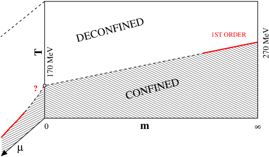
Figure 1: The Phase Diagram of $N_{f}=2$ QCD

A line exists across which $<L>,<\bar{\psi}\psi>,<E>$ all experience a rapid change, so that their susceptibilities have a peak. All these peaks happen to coincide within errors. Conventionally the phase below the line is called confined, the one above it deconfined. An order parameter is needed, which must exist if, as we have argued, the transition is order-disorder. The dual excitations have to be identified.

3 The dual excitations of QCD

The general idea is that the low temperature phase of QCD (strong coupling) can be described, in a dual language, in terms of topologically non trivial excitations which are non local in terms of gluons and quarks, but are local fields in a dual language, and weakly coupled[21][22][17].
There exist two main proposals for these excitations, both due to ’tHooft.

1) Vortices[21]

2) Monopoles[22],[23],[24].

In the vicinity of the deconfining transition $(T\leq T_{c})$ the free energy density should depend on the dual fields in a form dictated by symmetry and scale invariance. The deconfining transition is a change of symmetry : the disorder parameter $<\Phi_{dual}>\neq 0$ for $T<T_{c}$, $<\Phi_{dual}>=0$ for

$T\geq T_{c}$.
Two main approaches have been developed in the literature:
a) Expose in the lattice configurations the dual excitations and show that by removing them confinement gets lost. (Vortex dominance, abelian dominance, monopole dominance)
b) Study the symmetry and the change of symmetry across $T_{c}$.

3.1 Vortices

Vortices are one dimensional defects associated to closed lines $C$, $V(C)$. If $W(C^{\prime})$ is the Wilson loop, i.e. the parallel transport along the line $C^{\prime}$ then

$$V(C)W(C^{\prime})=W(C^{\prime})V(C)e^{i{{n_{CC^{\prime}}\pi}\over N_{c}}}$$ (25)

$n_{CC^{\prime}}$ is the linking number of the two curves $C,C^{\prime}$, which is well defined in $3d$.
In $(2+1)d$, $<V(C)>\neq 0$ means spontaneous breaking of a symmetry, the conservation of the number of vortices minus the number of anti-vortices, $<V(C)>=0$ means super-selection of that number, and $V(C)$ can be an order parameter for confinement. In $(3+1)d$ this statements have no special meaning.
In any case, as a consequence of Eq(3.1) whenever $V(C)$ obeys the area law $W(C^{\prime})$ obeys the perimeter law, and viceversa whenever $W(C^{\prime})$ obeys the area law $V(C)$ obeys the perimeter law.
The ’tHooft loop, defined as the expectation value of a vortex going straight across the lattice, or the dual of the Polyakov line, is non zero in the confined phase, zero in the deconfined phase[25]. The corresponding symmetry is $Z_{3}$, which, however, does not survive the introduction of dynamical quarks.

3.2 Monopoles

Monopoles exist as solitons in Higgs gauge theories with the Higgs in the adjoint representation [26][27]. They are stable for topological reasons.
If the gauge group is $SU(2)$ they are hedgehog-like configurations for the Higgs field $\phi$, with $\phi^{i}(\vec{r})\propto r^{i}$, and are characterized by a zero of $\phi$ corresponding to the position of the monopole. These configurations are called monopoles because of the non trivial topology of the mapping of the sphere at spacial infinity $S_{2}$ on the sphere of the possible values of $<\vec{\phi}>$.
Physically this can be understood in terms of the ’tHooft tensor, $F_{\mu\nu}$.

$$F_{\mu\nu}\equiv\hat{\phi}\vec{G}_{\mu\nu}-{1\over g}\hat{\phi}(D_{\mu}\hat{\phi}\wedge D_{\nu}\hat{\phi})$$ (26)

where $g$ is the gauge coupling constant, $D_{\mu}\hat{\phi}$ the covariant derivative of $\phi$,

$$D_{\mu}\hat{\phi}=[\partial_{\mu}-g\vec{A}_{\mu}\wedge]\hat{\phi}$$

and $\hat{\phi}\equiv{{\vec{\phi}}\over{|\vec{\phi}|}}.$
$F_{\mu\nu}$ is gauge invariant by construction. Moreover the bilinear terms in $A_{\mu}A_{\nu}$ cancel between the two terms of eq(3,2) and

$$F_{\mu\nu}=\partial_{\mu}(\hat{\phi}\vec{A}_{\nu})-\partial_{\nu}(\hat{\phi}\vec{A}_{\mu})-{1\over g}\hat{\phi}(\partial_{\mu}\hat{\phi}\wedge\partial_{\nu}\hat{\phi})$$

In the unitary gauge $\vec{\phi}=(0,0,1)$, the last term vanishes and

$$F_{\mu\nu}=\partial_{\mu}A^{3}_{\nu}-\partial_{\nu}A^{3}_{\mu}$$

an abelian field.
$F_{\mu\nu}$ obeys Bianchi identities

$$\partial_{\mu}F_{\mu\nu}^{*}=0$$ (27)

with $F_{\mu\nu}^{*}\equiv{1\over 2}\epsilon_{\mu\nu\rho\sigma}F_{\rho\sigma}$ the dual tensor. The identity can be violated at the location of singularities, where a non zero magnetic current exists

$$\partial_{\mu}F_{\mu\nu}^{*}\equiv j_{\nu}$$

In any case due to the antisymmetry of $F_{\mu\nu}^{*}$

$$\partial_{\nu}J_{\nu}=0$$ (28)

For the monopole solution [26]

$$F_{\mu 0}=0,(\vec{E}=0)$$

$${1\over 2}\epsilon_{ijk}F_{jk}={1\over{2g}}{r_{i}\over{r^{3}}}+Dirac-string$$

A Dirac monopole. The string is produced by the singularity of the transformation to the unitary gauge at the zero of $\phi$. The transformation to the unitary gauge is called Abelian Projection.
For $SU(N)$ gauge group one can inquire about the existence of monopole solitons and what the analog of $\hat{\phi}$ is[28]. If we denote by $\Phi=\Sigma_{a}\Phi^{a}T^{a}$ the Higgs field, by $A_{\mu}=\Sigma_{a}A^{a}_{\mu}T^{a}$ the gauge field and by $G_{\mu\nu}=\partial_{\mu}A_{\nu}-\partial_{\nu}A_{\mu}+ig[A_{\mu},A_{\nu}]$ the field strength tensor, with $T^{a}$ the generators of the gauge group in the fundamental representation, normalized as $Tr(T^{a}T^{b})=\delta^{ab}$,we can define the generalized ’tHooft tensor as

$$F_{\mu\nu}=Tr(\Phi G_{\mu\nu}-{i\over g}\Phi[D_{\mu}\Phi,D_{\nu}\Phi])$$ (29)

The necessary and sufficient condition to have abelian projection, i.e. cancellation of bilinear terms in $A_{\mu}A_{\nu}$ is that

$$\Phi=\Phi^{a},\Phi^{a}=U(x)^{\dagger}\Phi^{a}_{diag}U(x)$$

with U(x) an arbitrary gauge transformation and

$$\Phi^{a}_{diag}=diag({a\over N},{a\over N},...{a\over N}^{(N-a)times},-{{(N-a)}\over N},-{{(N-a)}\over N}....-{{(N-a)}\over N})a=1,2,....(N-1)$$ (30)

The residual symmetry is $SU(a)\otimes SU(N-a)\otimes U(1)$.
For each $\Phi^{a}$ one has

$$F_{\mu\nu}^{a}=Tr(\Phi^{a}G_{\mu\nu}-{i\over g}\Phi^{a}[D_{\mu}\Phi^{a},D_{\nu}\Phi^{a}])\\ =\partial_{\mu}Tr(\Phi^{a}A_{\nu})-\partial_{\nu}Tr(\Phi^{a}A_{\mu})-{i\over g}Tr(\Phi^{a}[\partial_{\mu}\Phi^{a},\partial_{\nu}\Phi^{a}])$$ (31)

Transforming to the unitary gauge where $\Phi^{a}=\Phi^{a}_{diag}$ gives

$$F_{\mu\nu}^{a}=\partial_{\mu}Tr(\Phi^{a}_{diag}A_{\nu})-\partial_{\nu}Tr(\Phi^{a}_{diag}A_{\mu})$$ (32)

Expanding the diagonal part of $A_{\mu}$ as a sum of simple roots of the algebra of the group, $\alpha^{a}$, which obey the orthogonality relations $Tr(\alpha^{a}\Phi^{b}_{diag})=\delta^{ab}$, $A^{\mu}_{diag}=\Sigma_{a}A^{a}_{\mu}\alpha^{a}$,one gets

$$F^{a}_{\mu\nu}=\partial_{\mu}A^{a}_{\nu}-\partial_{\nu}A^{a}_{\mu}$$ (33)

which is an abelian field. The simple roots have the form

$$\alpha^{a}=diag(0,0,....0,1,-1,0,...0)$$

with the 1 at the a-th entry. A monopole soliton solution exists for each value of $a$ in the $SU(2)$ subspace spanned by the elements $+1$ and $-1$. For the Higgs field one has

$$\Phi(x)=U(x)^{\dagger}\Phi(x)_{diag}U(x)$$

where $\Phi(x)_{diag}$ is defined with eigenvalues in decreasing order. Expanding $\Phi(x)_{diag}$ in the complete basis $\Phi^{a}_{diag}$,

$$\Phi(x)_{diag}=\Sigma_{a}c^{a}(x)\Phi^{a}_{diag}$$

one gets

$$\Phi(x)=\Sigma_{a}c^{a}(x)\Phi^{a}(x)$$ (34)

The transformation $U(x)$ is singular at the sites where some $c^{a}(x)$ vanishes, i.e. wherever two subsequent eigenvalues of $\Phi$ coincide: these points are the locations of the monopoles. The field strength $F^{a}_{\mu\nu}$ can be defined also in the absence of a Higgs field in the lagrangean simply as

$$F_{\mu\nu}^{a}=Tr(\Phi^{a}G_{\mu\nu}-{i\over g}\Phi^{a}[D_{\mu}\Phi^{a},D_{\nu}\Phi^{a}])$$ (35)

$${\Phi}^{a}(x)=U^{\dagger}(x)\Phi^{a}_{diag}U(x)$$ (36)

U(x) an arbitrary gauge transformation which can have non trivial topology or singular points.

$F^{a}_{\mu\nu}$ depends on the choice of $U(x)$. It obeys the Bianchi identities Eq.(3.3), apart from singularities where the magnetic current can be non zero.
In any case the magnetic current will obey the conservation law eq(3.4).
The theory has (N-1) topological symmetries built in, corresponding to the conservation of magnetic charges.
If these symmetries are realized a la Wigner the Hilbert space will be superselected. If they are Higgs broken the system will be a dual superconductor.
Our working hypothesis will be that the dual symmetry of QCD is the conservation of (N-1) magnetic charges.The change of symmetry at $T_{c}$ is a transition from Higgs-broken to superselected. Dual excitations carry magnetic charge.
Our program will then be to construct magnetically charged operators $\mu^{a}$ and study their vacuum expectation values $<\mu^{a}>$.
$<\mu^{a}>\neq 0$ means dual superconductivity.
$<\mu^{a}>=0$ means normal vacuum.
This should hold both in quenched theory and with dynamical quarks, in agreement with the ideas of $N_{c}\to\infty$ limit of QCD.

3.3 Construction of $<\mu^{a}>$

The basic idea is simply that

$$e^{ipa}|x>=|x+a>$$ (37)

if $x$ is a position variable and $p$ its conjugate momentum.
Specifically

$$\mu^{a}(\vec{x},t)=exp(i\int d^{3}yTr[\Phi^{a}(\vec{y},t)\vec{E}(\vec{y},t)]\vec{b}_{\perp}(\vec{x}-\vec{y}))$$ (38)

where $\vec{E}$ is the electric field operator, and $\vec{b}(\vec{x}-\vec{y})_{\perp}$ is the vector potential produced by a static monopole sitting at $\vec{x}$ in $\vec{y}$.

$$\vec{\nabla}\vec{b}_{\perp}=0,$$

$$\vec{\nabla}\wedge\vec{b}_{\perp}={2\pi\over g}{\vec{r}\over r^{3}}+Dirac-string$$

$$\Phi^{a}(x)=U^{\dagger}(x)\Phi^{a}_{diag}U(x)$$

with U(x) a generic gauge transformation.
$\mu^{a}$ is gauge invariant. In the gauge

$$\Phi^{a}=\Phi^{a}_{diag}$$

$$\mu^{a}(\vec{x},t)=exp(i\int Tr[\Phi^{a}_{diag}\vec{E}(\vec{y},t)]\vec{b}_{\perp}(\vec{x}-\vec{y})d^{3}y\\ =exp(i\int\vec{E}^{a}_{\perp}(\vec{y},t)\vec{b}_{\perp}(\vec{x}-\vec{y})d^{3}y$$ (39)

$\vec{E}^{a}_{\perp}(\vec{y},t)$ is the conjugate momentum to $\vec{A}^{a}_{\perp}(\vec{y},t)$ so that

$$\mu^{a}(\vec{x},t)|\vec{A}^{a}_{\perp}(\vec{y},t)>=|\vec{A}^{a}_{\perp}(\vec{y},t)+\vec{b}_{\perp}(\vec{x}-\vec{y})>$$ (40)

A Dirac monopole has been added to the abelian projected configuration. There are (N-1) species of monopoles, corresponding to a=1,….. N-1.
$\mu^{a}$ creates a singularity (monopole) in a selected gauge and in all the gauges obtained from it by a transformation which is continuous in a neighborhood of the singularity. The number of monopoles per $fm^{3}$ is finite as illustrated in Fig.2 where an histogram is displayed of the distribution of the difference between two eigenvalues of a plaquette operator for different values of the lattice spacing[29]. Therefore creating a monopole in an abelian projection implies that a monopole is also created in any other abelian projection, apart from a set of zero measure. The statements $<\mu^{a}>=0$ and $<\mu^{a}\neq 0>$ are independent of the abelian projection, so that the statement that QCD vacuum is or is not a dual superconductor are absolute, projection independent statements.

3.4 Measuring $<\mu^{a}>$

By construction

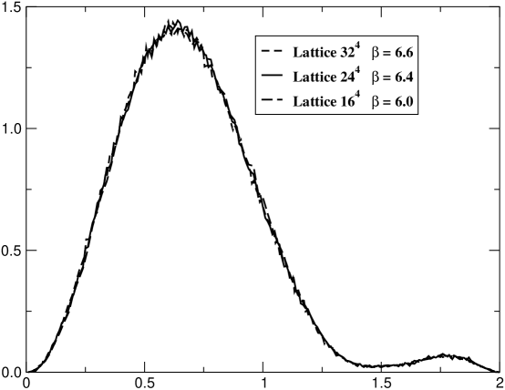
Figure 2: Distribution of the differences of the phases of the eigenvalues of the Polyakov line, for three lattices with the same physical volume and different lattice spacing. A monopole on any site would correspond to a non zero value at zero angle.

$$<\mu^{a}>={Z^{a}\over Z}$$ (41)

where $Z$ is the partition function of the theory, and $Z^{a}$ the one modified by the insertion of the monopoles. Eq(3.17) implies that at $\beta=0$ $<\mu^{a}>=1$.
Taking advantage of that it is convenient, instead of measuring $<\mu^{a}>$ directly, to measure its susceptibility $\rho^{a}={\partial\over\partial\beta}ln<\mu^{a}>$ which is much less noisy and will prove more suitable for our purposes. From Eq(3.17) one immediately gets

$$\rho^{a}=<S>_{S}-<S^{a}>_{S^{a}}$$ (42)

One also has

$$<\mu^{a}>=exp[\int d\beta^{\prime}\rho^{a}(\beta^{\prime})]$$ (43)

It follows from Eq(3.19) that, in the infinite volume limit :
(i) $<\mu^{a}>\neq 0$ for $T,T_{c}$ iff $\rho^{a}$ tends to a finite limit.
(ii) $<\mu^{a}>=0$ for $T>T_{c}$ iff $\rho^{a}\to\infty$ The property (ii) is much easier to check on $\rho$ than by a direct measurement of $<\mu>$ which can only give limits, due to statistical errors.
In the critical region $T\approx T_{c}$ a strong negative peak is expected due to a rapid decrease of $<\mu^{a}>$, and scaling laws corresponding to the fact that the correlation length goes large with respect to the lattice spacing. The renormalization group equations read[30]

$$<\mu^{a}>=L_{s}^{\kappa}\Phi^{a}(\tau L_{s}^{1\over\nu},mL_{s}^{y_{h}})$$ (44)

Sending $L_{s}\to\infty$ keeping $\tau L_{s}^{1\over\nu}$ fixed gives [30]

$$<\mu^{a}>\approx m^{{-\kappa}\over{y_{h}}}\phi^{a}(\tau L_{s}^{1\over\nu})$$

or

$$\rho^{a}/{L_{s}^{1\over\nu}}=f(\tau L_{s}^{1\over\nu})$$

a scaling law from which the critical index $\nu$ can be determined.
The prototype theory is compact $U(1)$ in $4d$, where everything is understood analytically at the level of theorems [14] [15][31]. There is a phase transition at $\beta_{c}\approx 1.01$ which is first order, from a confined phase to a deconfined phase, and $<\mu>$ is non zero below $\beta_{c}$ and zero above $\beta_{c}$.
Moreover $\mu$ is proved to be a gauge invariant charged operator of the Dirac type. A numerical determination provides a check of the approach. The result is shown in Fig.s 3,4,5

Figure 3: $\rho$ vs $\beta$. The peak signals the transition

A strong negative peak signals the transition. At low $\beta^{\prime}s$ $\rho$ is size independent, at large $\beta^{\prime}s$ it is proportional to $L_{s}$ with a negative coefficient, implying that $<\mu>$ is strictly zero in the thermodynamic limit.

Figure 4: Size dependence of $\rho$ below $\beta_{c}$

Finite size scaling agrees with a first order transition.

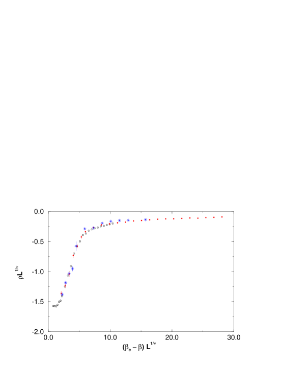
Figure 5: Finite size scaling.

For quenched $SU(2)$ theory the deconfining transition is detected in a similar way at the right value of $\beta$ and the critical index $\nu$ is that of the $3d$ ising model[32].

Quenched $SU(3)$ also shows a first order transition at the right temperature [33].

The numerical check of the independence on the choice of the abelian projection is contained in [34].

The case of $N_{f}=2$ $QCD$ can be approached in the same way. The results are displayed in the Fig.’s6, 7,8, 9. The finite size scaling is that of a first order transition, and definitely excludes a second order transition in the universality class of O(4), O(2) model[29].

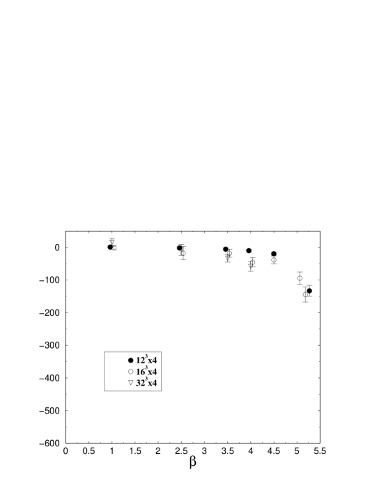
Figure 6: $N_{f}=2$.Size dependence of $\rho$ below $\beta_{c}$

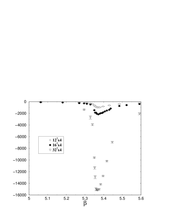
Figure 7: $\rho$ peaks at different spatial sizes.

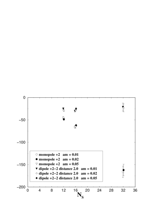
Figure 8: $\rho$ tends to $-\infty$ in the thermodynamical limit, or $<\mu>\to 0$

The implications of this fact, together with a finite size scaling analysis of other quantities, like the specific heat, the chiral condensate and its susceptibility will be the object of the next section.

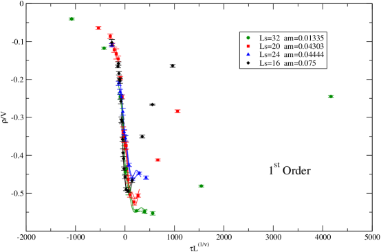
Figure 9: Scaling of $\rho$ consistent with a first order transition.

4 $N_{f}=2$ QCD

QCD with two flavors of light quarks is a good approximation to nature, and also a specially instructive system from the theoretical point of view. For the sake of simplicity we shall consider two quarks of equal mass $m$.
The phase diagram is shown in Fig.1. For $m\geq 2Gev$ the system is quenched to all effects, the phase transition is first order and $<L>$ is a good order parameter, $Z_{3}$ the relevant symmetry. At $m\approx 0$ a phase transition takes place from the spontaneously broken phase to a symmetric phase, and $<\bar{\psi}\psi>$ is the order parameter. In the intermediate region of $m$’s chiral symmetry is broken by the mass, $Z_{3}$ is broken by the coupling to quarks and apparently there is no order parameter. Also The $U_{A}(1)$ symmetry which is broken by the anomaly is expected to be restored about at the same temperature as the chiral symmetry. Three transitions, deconfinement, chiral, $U_{A}(1)$: are they independent? Of course a definition of deconfinement is needed to answer this question.

4.1 The Chiral Transition

If one assumes, following reference [35] that low mass scalars and pseudoscalars are the relevant degrees of freedom, the order parameters are

$$\underline{\Phi}:\Phi_{ij}=<\bar{\Psi}_{i}(1+\gamma_{5})\Psi_{j}>\,,i,j=1...N_{f}$$ (45)

Under the symmetry group $SU(N_{f})\otimes SU(N_{f})\otimes U_{A}(1)$

$$\Phi\to e^{i\alpha}U_{L}\Phi U_{R}$$

. The most general effective Lagrangean (density of free energy) invariant under the symmetry group is

$$L_{eff}={1\over 2}Tr(\partial_{\mu}\Phi^{\dagger}\partial_{\mu}\Phi)-{m^{2}\over 2}Tr(\Phi^{\dagger}\Phi)-{{\pi}^{2}\over 3}g_{1}[Tr(\Phi^{\dagger}\Phi)]^{2}-{{\pi}^{2}\over 3}g_{2}[Tr(\Phi^{\dagger}\Phi)^{2}]+\\ c[det{\Phi}+det{\Phi}^{\dagger}]$$ (46)

Terms with higher dimension have been neglected since they become irrelevant at the critical point.
Infrared stable fixed points indicate second order phase transitions. A $(4-{\epsilon})$ extrapolation to $3d$ is intended. The last term in Eq(4.2) is the Wess-Zumino term describing the anomaly: it is invariant under $SU(N_{f})\otimes SU(N_{f})$ but not under $U_{A}(1)$, and has dimension $N_{f}$. For $N_{f}\geq 3$ it is irrelevant and no IR stable fixed point exists, so that the transition is weak first order.
For $N_{f}=2$ instead the Wess-Zumino term has dimension $2$ so that its square and its product with the mass term are also relevant. If $c=0$ at the fixed point the symmetry is $O(4)\otimes O(2)$ and no IR fixed point exists, so that the transition is 1st order. Physically this happens if the mass of the $\eta\prime$, $m_{\eta\prime}$, vanishes at $T_{c}$.
If $c\neq 0$, or if $m_{\eta\prime}$ is non zero at $T_{c}$, the symmetry is $O(4)$ and the transition can be second order. If this is the case the transition is a crossover around the critical point [see Fig. 1], a tricritical point is expected at non zero chemical potential [36] which could be observed in heavy ion collisions. No evidence of it has emerged from experiments to date.
If, instead, the transition is first order it will also be such in the vicinity of the chiral point and possibly all along the transition line, and no tricritical point exists.
This issue is fundamental to understand confinement: a first order phase transition is a real transition and can correspond to a change of symmetry and to the existence of an order parameter.
A crossover means that one can go continuously from the confined region to the deconfined one and that confinement is not an absolute property of the QCD vacuum.

4.2 Thermodynamics

The order of the transition can be determined by a finite size scaling analysis [37][38] of lattice simulations.
Let $\tau=(1-{T\over T_{c}})$ be the reduced temperature. As $\tau\to 0$ the correlation length of the order parameter, $\xi$, diverges as

$$\xi\approx\tau^{-\nu}$$

so that the ratio of the lattice spacing $a$ to $\xi$ is negligible and there is scaling. If $L_{s}$ is the spacial extension of the lattice, the scaling laws read

$$C_{V}-C_{0}\approx L_{s}^{\alpha\over\nu}\Phi_{C}(\tau L_{s}^{1\over\nu},mL_{s}^{y_{h}})$$ (47)

and

$$\chi\approx L_{s}^{\gamma\over\nu}\Phi_{\chi}(\tau L_{s}^{1\over\nu},mL_{s}^{y_{h}})$$ (48)

Here $C_{V}={{\partial E}\over{\partial T}}_{V}$, and

$$\chi\equiv\int d^{3}x<\Phi(\vec{x})\Phi(\vec{0})>_{conn}$$

is the susceptibility of the order parameter $\Phi$.
The critical indexes $\alpha,\beta,\gamma,\nu$ are the anomalous dimensions of the operators and identify the order and the universality class of the transition. Eq’s(4.3) and (4.4) are nothing but the renormalization group equations. The subtraction needed for $C_{V}$ corresponds to an additive renormalization[38].
Notice that the scaling law of the specific heat is unambiguous whilst that for $\chi$ only holds if $\Phi$ is the order paramenter : the equality of the index ${\nu}$ for the two scalings can a legitimation of the order parameter.
The scaling laws Eq.’s(4.3) and (4.4) involve two scales, a fact which makes the analysis complicated with respect to the simpler case of quenched QCD. To simplify the problem one can study the dependence on one scale by keeping the other one fixed [30]. One possibility is to vary $m$ and $L_{s}$ keeping the quantity $mL_{s}^{1\over\nu}$ which appears in the scaling laws fixed. The scaling equation (4.3) becomes then

$$C_{V}-C_{0}\approx L_{s}^{\alpha\over\nu}\Phi_{C}(\tau L_{s}^{1\over\nu},mL_{s}^{y_{h}}=M)$$ (49)

so that the peak scales as

$$(C_{V}-C_{0})_{peak}\propto L_{s}^{\alpha\over\nu}$$ (50)

This allows a determination of ${\alpha\over\nu}$. The critical index $y_{h}$ is the same within errors for $O(4)$ and $O(2)$ universality classes, so that the same simulations can be used to check both universality classes; moreover the index $\alpha$ is negative for both, implying that the peak should decrease with increasing volume. (see Table 1)

	$y_{h}$	$\nu$	$\alpha$	$\gamma$	$\delta$
$O(4)$	2.487(3)	0.748(14)	-0.24(6)	1.479(94)	4.852(24)
$O(2)$	2.485(3)	0.668(9)	-0.005(7)	1.317(38)	4.826(12)
$MF$	$9/4$	$2/3$	0	1	3
$1^{st}Order$	3	$1/3$	1	1	$\infty$

Table 1: Critical exponents.

Fig.10 shows a test of Eq(4.5),Fig.12 a test of Eq(4.6). $O(4)$ and $O(2)$ universality classes are excluded with a high confidence level ($\chi^{2}/dof\simeq 20$) : the peaks increase rapidly with the volume instead of decreasing.

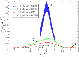
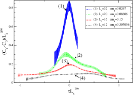
Figure 10: Test of scaling Eq.(4.5), with $M=74.7$ (left) and $M=149.4$(right) : the curves should coincide.

For the details of the determination of the subtraction $C_{0}$ see [30].

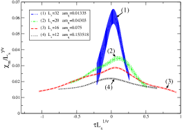
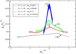
Figure 11: Scaling Eq.(4.7) of the chiral susceptibility, with $M=74.7$ (left) and $M=149.4$ (right) : the curves should coincide.

A similar result is obtained for the susceptibility of $<\bar{\psi}\psi>$ which is believed to be a good order parameter near $T_{c}$ (Fig.11 and Fig. 12)

$$\chi\approx\Phi_{\chi}(\tau L_{s}^{1\over\nu},mL_{s}^{y_{h}}=M)$$ (51)

and

$$\chi_{peak}\propto L_{s}^{\gamma\over\nu}$$ (52)

For this test $\chi^{2}/dof\approx 10$.

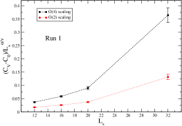
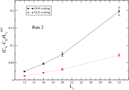
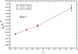
Figure 12: Test of the scaling Eq.’s (4.6) and (4.8)

As a result we can state that the transition is neither in the universality class of $O(4)$ nor in that of $O(2)$. Another possibility is to look at the large volume limit keeping the first variable fixed: $\tau L_{s}^{1\over\nu}$ is related to the ratio ${\xi\over L_{s}}$ of the correlation length to the spacial size of the lattice, while the other variable $mL_{s}^{y_{h}}$ is related to the ratio of the pion Compton wave length ${1\over{m_{\pi}}}$ to $L_{s}$. As $L_{s}$ goes much larger than ${1\over{m_{\pi}}}$ a finite limit is reached and[30]

$$C_{V}-C_{0}\approx m^{{-\alpha}\over{\nu y_{h}}}f_{C}(\tau L_{s}^{1\over\nu})$$ (53)

and

$$\chi\approx m^{\gamma\over{\nu y_{h}}}\Phi_{\chi}(\tau L_{s}^{1\over\nu})$$ (54)

The result of this analysis is shown in Fig.13and Fig14. No scaling is observed assuming second order transition with $O(4)$ or $O(2)$, but a good scaling for first order.

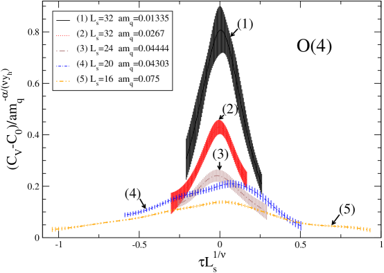
Figure 13: Scaling Eq.(4.9) for O(4).

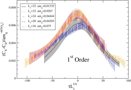
Figure 14: Scaling Eq.(4.9) for first order.

A similar result is obtained for the scaling Eq.(4.10) Fig.15

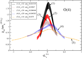
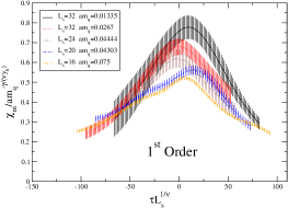
Figure 15: Testing Eq.(4.10) for O(4) and first order.

Finally one can investigate the so called magnetic equation of state:

$$<\bar{\psi}\psi>=m^{1\over\delta}f(\tau m^{-1\over{\nu y_{h}}})$$ (55)

For $O(4)$ $\delta=4.85$, for first order $\delta=\infty$ Again no scaling is observed assuming $O(4)$ or $O(2)$ second order transition Fig.16, and good scaling for first order, Fig17.

The issue is fundamental and deserves further attention.

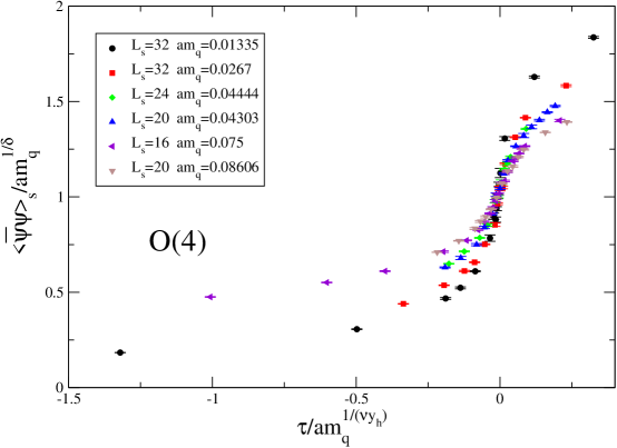
Figure 16: Scaling of the magnetic equation of state (4.11) assuming O(4)

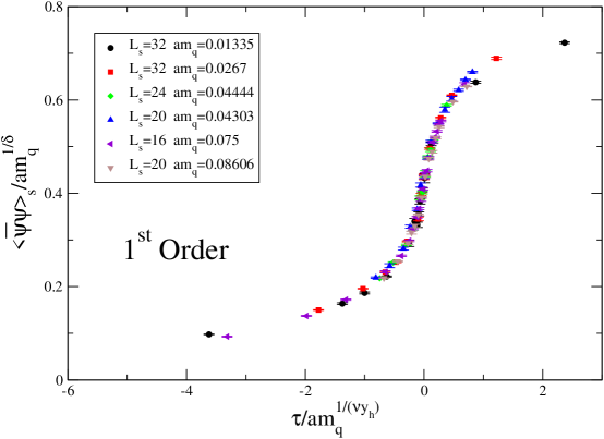
Figure 17: Scaling of the magnetic equation of state (4.11) assuming first order

5 Concluding remarks

We have discussed the experimental evidence for confinement and how it naturally implies that there exists a dual symmetry in QCD whose breaking is responsible for confinement. We have presented the two most accredited candidates for dual topological excitations, vortices and monopoles.
We have then shown how the working hypothesis that monopoles confine via dual superconductivity of the vacuum can be tested by numerical simulations on the lattice, through an order parameter which is the $vev$ of operators carrying magnetic charge. The numerical tests strongly support the validity of this idea, which can be put in a consistent form and made independent on the choice of the abelian projection. This holds both for quenched QCD and in the presence of dynamical quarks.
A prerequisite is that deconfinement is a true order-disorder phase transition, and not a crossover, which would allow a continuous path from confined to deconfined phase. We have thus discussed a test with $N_{f}=2$ QCD where an unsolved dilemma exists between the existence of a crossover and a first order phase transition. We definitely exclude a second order chiral transition which would imply a crossover at non zero quark mass, whilst we find evidence for a first order transition. The issue is fundamental and deserves further studies.
From what we have seen we can conclude that the dual excitations of $QCD$ are magnetically charged, or that dual superconductivity of the vacuum can be the mechanism of confinement.
However we are not yet able to identify them.

References

- [1] M. Gell-mann:Phys.Lett.8 (1964) 214
- [2] R.P.Feynman, M. Gell-Mann :Phys.Rev.109 (1958) 193
- [3] M. Gell-Mann:Phys. Rev.125 (1962) 1067
- [4] M. Gell-Mann:Acta Phys. Austriaca Suppl.9 (1972) 733
- [5] H. Fritzsch, M. Gell-Mann, H. Leutwyler:Phys.Lett.47B (1973) 365
- [6] Review of Particle Physics:EPJ15 (2000)
- [7] L. Okun: Leptons and Quarks, North Holland (1982)
- [8] R. Hagedorn: Nuovo Cim. Suppl. 3 (1965) 147
- [9] N. Cabibbo, G. Parisi: Phys. Lett.59B (1975) 67
- [10] H.A. Kramers, G.H. Wannier:Phys. Rev.60 (1941) 252
- [11] L.P.Kadanoff, H. Ceva:Phys. Rev. B3 (1971) 3918
- [12] G. Di Cecio, A. Di Giacomo, G. Paffuti, A. Trigiante:Nucl. Phys. B489 (1997) 739
- [13] A. Di Giacomo, D. Martelli, G. Paffuti:Phys. Rev. D60(1999) 094511
- [14] J. Froelich, P.A.Marchetti:Commun. Math. Phys. 112 (1987) 343
- [15] A. Di Giacomo, G. Paffuti: Phys. Rev. D56 (1997) 6816
- [16] V. Cirigliano, G. Paffuti: Commun. Math. Phys.200 (1999) 381
- [17] N. Seiberg, E. Witten :Nucl. Phys. B 341 (1994) 484
- [18] T. Banks, W. Fischler, S. H. Shenker, L. Susskind:Phys. Rev. D55 (1997) 5112
- [19] O. Kaczmarek, F. Karsch, P. Petreczky, F. Zantow:Nucl. Phys. Proc Suppl. B129 (2004) 560
- [20] Finite size scaling, J.L.Cardy ed. North Holland (1988)
- [21] G. ’tHooft:Nucl. Phys.B138 (1978) 1
- [22] G. ’tHooft:Nucl. Phys.B190 (1981) 455
- [23] G. ’tHooft :High Energy Physics EPS International Conference Palermo 1975,A. Zichichi ed.
- [24] S. Mandelstam:Phys. Repts23C (1976) 245
- [25] L. Del Debbio, A. Di Giacomo, B. Lucini:Nucl. Phys.bf B594 (2001) 287
- [26] G. ’tHooft:Nucl. Phys.B79 (1974) 276
- [27] A. M. Polyakov:Pis’ma JETP20 (1974) 430
- [28] L.Del Debbio, A. Di Giacomo, B. Lucini, G. Paffuti. Abelian projection in SU(N) gauge theories hep-lat/0203023
- [29] M. D’Elia, A. Di Giacomo, B. Lucini, G. Paffuti, C. Pica:Phys. Rev.D71 (2005) 114502
- [30] M. D’Elia, A. Di Giacomo, C. Pica:hep-lat/0503030 Submitted for publication.
- [31] A. Di Giacomo, G. Paffuti:Nucl. Phys. Proc. Suppl.106( 2002) 664
- [32] A. Di Giacomo, B. Lucini, L. Montesi, G. Paffuti :it Phys. Rev. D61(2000)034503
- [33] A. Di Giacomo, B. Lucini, L. Montesi, G. Paffuti :it Phys. Rev. D61(2000)034504
- [34] J.Carmona,M. D’Elia, A. Di Giacomo, B. Lucini, G. Paffuti:Phys. Rev. D64(2001)114507
- [35] R.D.Pisarski, F.Wilczek:Phys.Rev. D29, (1984) 338
- [36] M.A. Stephanov, K.Rajagopal, E.V. Shuryak:Phys. Rev. Lett. 81 (1998) 4816
- [37] M.E.Fischer, M.N. Barber:Phys. Rev. Lett.28 (1972) 1516
- [38] E. Brezin :Journal de Physique 43 (1982) 15
- [39] K.G.Wilson: Phys. Rev. D10 (1974) 2445