HMC algorithm with multiple time scale integration and mass preconditioning

Abstract:

We describe a new HMC algorithm variant we have recently introduced and extend the published results by preliminary results of a simulation with a pseudo scalar mass value of $m_{\mathrm{PS}}\approx 300\ \mathrm{MeV}$. This new run confirms our expectation that simulations with such pseudo scalar mass values become feasible and affordable with our HMC variant. In addition we discuss simulations from hot and cold starts at $m_{\mathrm{PS}}\approx 300\ \mathrm{MeV}$, which we performed in order to test for possible meta-stabilities.

PoS(LAT2005)118

1 Introduction

Even though Wilson’s original discretization of the Dirac operator gives rise to one of the clearest and best understood formulations of lattice QCD, it shows problems in practice: due to explicit chiral symmetry breaking the Wilson operator develops unphysically small eigenvalues, which were thought to be responsible for instabilities observed in dynamical simulations at light values of the quark masses with the Hybrid Monte Carlo (HMC) algorithm [1].

However, recently it was discovered that – rather surprisingly – stable simulations with the HMC algorithm are possible with values of the pseudo scalar mass $m_{\mathrm{PS}}$ as low as $380\ \mathrm{MeV}$ [2, 3], if a clever combination of fermion determinant preconditioning and multiple time scale integration is used. Moreover, the computational costs appear to be affordable, even with $m_{\mathrm{PS}}\approx 300\ \mathrm{MeV}$, if the available results for the computational costs are extrapolated to this value of $m_{\mathrm{PS}}$.

In this proceeding we report on progress with the HMC variant we introduced in ref. [3].

2 Mass preconditioning

For simplicity we consider here $N_{f}=2$ mass degenerate flavors of Wilson fermions with Wilson-Dirac operator $D_{\mathrm{W}}$ and the Wilson plaquette gauge action $S_{\mathrm{g}}$. The lattice action (for one flavor) reads

$$S=S_{\mathrm{g}}+\sum_{x}\bar{\psi}(x)(D_{\mathrm{W}}+m_{0})\psi(x)\,,$$ (1)

where $m_{0}$ is the bare quark mass. For convenience we also introduce the hopping parameter $\kappa=(2am_{0}+8)^{-1}$ and the hermitian Wilson-Dirac operator $Q=\gamma_{5}D_{\mathrm{W}}$.

The numerical integration in the molecular dynamics part of the HMC algorithm [1] is usually performed by means of the leap-frog algorithm, which is reversible and area preserving, properties that are needed for the HMC algorithm to be exact. We refer to ref. [3] for details on how the leap frog algorithm is generalized to multiple time scales. In that reference we also detail how to generalize the so-called Sexton-Weingarten (SW) improved integration scheme [5].

While the HMC variant presented in ref. [2] is based on domain decomposition preconditioning, our variant relies on the so-called Hasenbusch acceleration or mass preconditioning [6]. It was realized in ref. [6] that using the identity

$$\det Q^{2}=\det\left(Q^{2}+\mu^{2}\right)\ \det\left(\frac{Q^{2}}{Q^{2}+\mu^{2}}\right)$$ (2)

with a mass shift $\mu$ can speed up the HMC algorithm, if each of the two determinants on the r.h.s. of eq. (2) is treated by a separate pseudo fermion field $\phi_{i}$ and a corresponding pseudo fermion action $S_{\mathrm{PF}_{i}}$. The acceleration comes about for the following reason: the condition number of $Q^{2}+\mu^{2}$ and $Q^{2}/(Q^{2}+\mu^{2})$ is reduced when compared to the condition number of $Q^{2}$. A reduced condition number is expected to lead to a reduced molecular dynamics force and hence allows for larger step sizes in the integration. At the same time the inversion of $Q^{2}+\mu^{2}$ is – due to the mass shift – much cheaper than the inversion of $Q^{2}$, altogether leading to a net speed up.

The original idea was then to choose the mass shift $\mu$ such that the condition numbers of $Q^{2}+\mu^{2}$ and $Q^{2}/(Q^{2}+\mu^{2})$ become approximately equal. The speed-up was observed to be around a factor of two [7].

3 HMC with multiple time scale integration and mass preconditioning

Motivated by the successful combination of multiple time scale integration and determinant preconditioning via domain decomposition in ref. [2], we explored in ref. [3] the idea of combining mass preconditioning with multiple time scale integration. With mass preconditioning the Hamiltonian for the HMC algorithm reads

$$H=\frac{1}{2}\sum_{x,\mu}P_{x,\mu}^{2}+\sum_{i=0}^{k}S_{\mathrm{PF}_{i}}\,.$$ (3)

The strategy is then to tune $\mu$ in eq. (2) such that the more expensive the computation of a certain $\delta S_{\mathrm{PF}_{i}}$ is, the less it contributes to the total force. The different parts of the action can then be integrated on different time scales $\Delta\tau_{i}$ chosen according to their force magnitude $F_{i}$, guided by $\Delta\tau_{i}F_{i}=\mathrm{const}$ for all $i$.

In ref. [3] we demonstrated that this idea proves to be useful in practice: we compared the performance of our HMC algorithm variant to the variant of ref. [2] and to a plain HMC as used in ref. [8]. The simulations were done on $24^{3}\times 32$ lattices with $\beta=5.6$ and pseudo scalar masses of $m_{\mathrm{PS}}=665\ \mathrm{MeV}$, $485\ \mathrm{MeV}$ and $380\ \mathrm{MeV}$ (runs $A$, $B$ and $C$). Details for the algorithm parameters as well as results for several quantities such as the plaquette expectation value or the vector mass $m_{\mathrm{V}}$ can be found in ref. [3]. In addition to these published results we have one more simulation point, corresponding to $m_{\mathrm{PS}}=294\ \mathrm{MeV}$ [9] (run $D$). Our simulations at this point are still ongoing and the history of this run is not yet long enough to be fully conclusive. Nevertheless, we present here first performance results for this point.

The first important observation from our investigations is that for all four aforementioned simulation points the preconditioning masses and time scales can be tuned such that simulations are stable. Examples for Monte Carlo histories of the plaquette expectation value or $\Delta H$ can be found in ref. [3].

In order to compare the performance of our HMC variant to other variants we have chosen two different measures. The first is the performance figure $\nu=10^{-3}(2n+3)\tau_{\mathrm{int}}(P)$ as introduced in ref. [2]. $\tau_{\mathrm{int}}(P)$ is the integrated autocorrelation time of the plaquette and $n$ is the number of integration steps for the physical operator $Q^{2}$ necessary for one trajectory. $\nu$ represents the number of inversions of the operator $Q$ in thousands needed in order to obtain one independent configuration. It is clearly algorithm and machine independent, but it does not account for the preconditioning overhead, which is at least for our HMC variant not completely negligible.

$\bigl{.}\Bigr{.}$	$\kappa$	$\nu$ $[$this work$]$	$\nu$[2, 9]	$\nu$[8]
$A$	$0.15750$	$0.09(3)$	$0.69(29)$	$1.8(8)$
$B$	$0.15800$	$0.11(3)$	$0.50(17)$	$5.1(5)$
$C$	$0.15825$	$0.23(9)$	$0.62(23)$	-
$D$	$0.15835$	red$0.35$	$0.74(18)$	-

Table 1: Comparison of $\nu$ values from this work, ref. [2] (with updates from [9]) and ref. [8].

The results for the $\nu$-values are summarized in table 1 and, while the $\nu$-values for our HMC variant and the one of ref. [2, 9] are compatible, they are significantly smaller than the values extracted for the plain HMC algorithm used in ref. [8]. Note that our $\nu$-value for simulation point $D$ (in red) is only based on an extrapolation of $\tau_{\mathrm{int}}(P)$ in $1/m_{\mathrm{PS}}^{2}$ and therefore preliminary.

The second performance measure we used is the number of floating point operations (flops) needed to generate $1000$ independent configurations of size $24^{3}\times 40$ with $a\approx 0.08\ \mathrm{fm}$. For this measure we could compare our HMC variant to the cost formula of ref. [10]

$$C=K\left(\frac{m_{\mathrm{PS}}}{m_{\mathrm{V}}}\right)^{-4}L^{5}a^{-7}\,.$$ (4)

The actual value of $K$ can be found in [10]. The result of the comparison is shown in figure 1 as an update of the “Berlin Wall” figures of [10, 11]. In figure 1(a) we compare our results represented by squares to the results of ref. [8] represented by circles. The lines are functions proportional to $(m_{\mathrm{PS}}/m_{\mathrm{V}})^{-4}$ (dashed) and $(m_{\mathrm{PS}}/m_{\mathrm{V}})^{-6}$ (solid) with a coefficient such that they cross the data points corresponding to the lightest pseudo scalar mass. The diamond represents the preliminary result of simulation point $D$, where the values for $\tau_{\mathrm{int}}(P)$ and $m_{\mathrm{V}}$ are extrapolated.

In figure 1(b) we compare to the formula of eq. 4 [10] (solid line) by extrapolating our data with $(m_{\mathrm{PS}}/m_{\mathrm{V}})^{-4}$ (dashed) and with $(m_{\mathrm{PS}}/m_{\mathrm{V}})^{-6}$ (dotted), respectively. The arrow indicates the physical pion to rho meson mass ratio. Additionally, we add points from staggered fermion simulations as were used for the corresponding plot in ref. [11]. Note that all the cost data were scaled to match a lattice time extend of $T=40$.

The most important conclusion from figure 1 is that with our HMC variant the “Wall” is substantially shifted towards smaller values of the quark mass and that simulations with Wilson fermions and $m_{\mathrm{PS}}\lesssim 300\ \mathrm{MeV}$ become feasible. Although the result for simulation point $D$ is preliminary, it nicely confirms the results for larger values of $m_{\mathrm{PS}}$, even under the pessimistic assumption that the final value might be a factor of two larger.

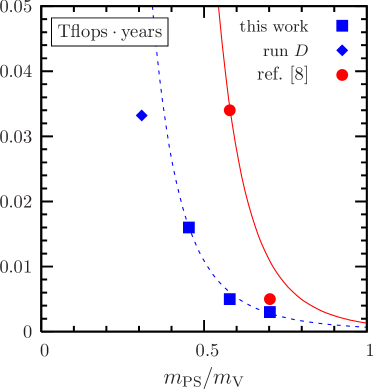
(a) Comparison to ref. [8].

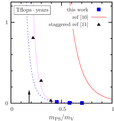
(b) Update of the “Berlin Wall” plots of refs. [10, 11].

Figure 1: Computer resources needed to generate $1000$ independent configurations of size $24^{3}\times 40$ at a lattice spacing of about $0.08\ \mathrm{fm}$ in units of $\mathrm{Tflops}\cdot\mathrm{years}$ as a function of $m_{\mathrm{PS}}/m_{\mathrm{V}}$. (See text for details.)

4 Thermalization property or meta-stability?

Dynamical Wilson fermion simulations show the generic property of a first order phase transition at the chiral point, as was shown in ref. [12]. At this phase transition point the PCAC quark mass jumps from non-vanishing negative to positive values (or vice versa) and the pseudo scalar mass assumes a non-zero minimal value, which can be rather large. This minimal value is supposed to vanish as $a^{2}$ towards the continuum limit, but a reliable information at which value of $a$ it takes a value below, say, $300\ \mathrm{MeV}$, is missing. In ref. [13] this value of $a$ was estimated to be around $0.1-0.07\ \mathrm{fm}$.

Since simulation point $D$ has $m_{\mathrm{PS}}\approx 300\ \mathrm{MeV}$ and the value of $a$ lies in the aforementioned interval, it is important to investigate whether at this simulation point a meta-stability is observed. To this end we performed for simulation point $D$ two simulations, one started from an ordered and the other from a disordered configuration. Both of these two runs reached now a Monte Carlo history of about $1000$ trajectories, but it is still not completely clear whether the runs have thermalized.

Nevertheless, when measuring the PCAC quark mass for both runs during the thermalization we observe that the run which started from a disordered configuration shows a positive value of this quantity while the other run has a negative value, indicating a meta-stability as observed in ref. [12]. Only after around $900$ trajectories the results of both runs approach each other and seem to converge to a positive value of the quark mass. Hence, it seems that at these parameter values no meta-stability occurs and the observed signs are simply thermalization effects. Nevertheless, this observation emphasizes the importance of checking for meta-stabilities before large scale simulations are started. It might also indicate that simulation point $D$ is close to a first order phase transition that possibly occurs at lower values of $m_{\mathrm{PS}}$.

5 Conclusion

In this proceeding we have reported on our progress with a new variant of the HMC algorithm, which we introduced in ref. [3]. The performance of our variant is comparable to the recently introduced HMC variant with domain decomposition [2] and clearly superior to a plain HMC algorithm. We presented an update of the “Berlin Wall” figure of refs. [10, 11] showing that with our HMC variant simulations with $m_{\mathrm{PS}}\approx 300\ \mathrm{MeV}$ become affordable and do not suffer from instabilities.

Moreover, we presented results of a check for meta-stabilities at our simulation point with the lowest value of $m_{\mathrm{PS}}$. We observed signs for a meta-stability during thermalization, which disappear only after around $1000$ trajectories.

For the future it would be interesting to understand why the two HMC algorithm variants – the ones discussed here and in ref. [2] – allow for stable simulations with values of the pseudo scalar mass of about $300\ \mathrm{MeV}$. One speculation is that this is due to the infrared regularization of the operator spectrum provided by both, mass and domain decomposition preconditioning. Another speculation is that the determinant and the forces are not well enough estimated with only one pseudo fermion field, leading to possibly large fluctuations in the forces. These fluctuations can be reduced by introducing additional pseudo fermion fields.

Clearly the clarification of these possibilities would be very interesting and it might provide important insight to even further improve the HMC algorithm.

Acknowledgments

We thank I. Montvay and I. Wetzorke helpful discussions, the $qq+q$ collaboration and in particular F. Farchioni, I. Montvay and E.E. Scholz for providing us their analysis program for the masses and C. Destri and R. Frezzotti for giving us access to a PC cluster in Milano. We also thank the computer-centers at HLRN and at DESY Zeuthen for granting the necessary computer-resources, and M. Hasenbusch for leaving us his HMC code as a starting point. This work was supported by the DFG Sonderforschungsbereich/Transregio SFB/TR9-03.

References

- [1] S. Duane, A. D. Kennedy, B. J. Pendleton and D. Roweth, Hybrid monte carlo, Phys. Lett. B195 (1987) 216–222.
- [2] M. Lüscher, Schwarz-preconditioned HMC algorithm for two-flavour lattice QCD, Comput. Phys. Commun. 165 (2005) 199 [hep-lat/0409106].
- [3] C. Urbach, K. Jansen, A. Shindler and U. Wenger, HMC algorithm with multiple time scale integration and mass preconditioning, hep-lat/0506011. Accepted for publication in Comput. Phys. Commun.
- [4] M. A. Clark and A. D. Kennedy, Accelerating fermionic molecular dynamics, hep-lat/0409134.
- [5] J. C. Sexton and D. H. Weingarten, Hamiltonian evolution for the hybrid monte carlo algorithm, Nucl. Phys. B380 (1992) 665–678.
- [6] M. Hasenbusch, Speeding up the Hybrid-Monte-Carlo algorithm for dynamical fermions, Phys. Lett. B519 (2001) 177–182 [hep-lat/0107019].
- [7] M. Hasenbusch and K. Jansen, Speeding up lattice QCD simulations with clover-improved Wilson fermions, Nucl. Phys. B659 (2003) 299–320 [hep-lat/0211042].
- [8] B. Orth, T. Lippert and K. Schilling, Finite-size effects in lattice QCD with dynamical wilson fermions, Phys. Rev. D72 (2005) 014503 [hep-lat/0503016].
- [9] M. Lüscher, Lattice QCD with light Wilson quarks, PoS(LAT2005)002 (2005) [hep-lat/0509152].
- [10] CP-PACS and JLQCD Collaboration, A. Ukawa, Computational cost of full QCD simulations experienced by CP-PACS and JLQCD Collaborations, Nucl. Phys. Proc. Suppl. 106 (2002) 195–196.
- [11] K. Jansen, Actions for dynamical fermion simulations: Are we ready to go?, Nucl. Phys. Proc. Suppl. 129 (2004) 3–16 [hep-lat/0311039].
- [12] F. Farchioni et. al., Twisted mass quarks and the phase structure of lattice QCD, Eur. Phys. J. C39 (2005) 421–433 [hep-lat/0406039].
- [13] F. Farchioni et. al., Lattice spacing dependence of the first order phase transition for dynamical twisted mass fermions, hep-lat/0506025. Accepted for publication in Phys. Lett. B.