Anatomy of string breaking in QCD

Abstract:

We investigate the string breaking mechanism in $n_{f}=2$ QCD. We discuss the lattice techniques used and present results on energy levels and mixing angle of the static $B\overline{B}|\overline{Q}Q$ two-state system. The string breaking is visualized, by means of an animation of the action density distribution as a function of the static colour source-antisource separation.

PoS(LAT2005)308

1 Introduction

The breaking of the colour-electric string between two static sources is a prime example of a strong decay in QCD [1]. Recently, we reported on an investigation of this two state system [2, 3], with a wave function $|Q\rangle$ created by a $\overline{Q}Q$ operator and a wave function $|B\rangle$ created by a four-quark $B\overline{B}$ operator, where $B=\overline{Q}q$. $Q$ denotes a static source and $q$ is a light quark. We determined the energy levels $E_{1}(r)-2m_{B}$ and $E_{2}(r)-2m_{B}$ of the two physical eigenstates $|1\rangle$ and $|2\rangle$ which we decomposed into the components,

$$|1\rangle = \cos{\theta}\,|Q\rangle+\sin{\theta}\,|B\rangle$$ (1)

$$|2\rangle = -\sin{\theta}\,|Q\rangle+\cos{\theta}\,|B\rangle.$$ (2)

We characterize string breaking by the distance scale $r_{c}$ at which $\Delta E=E_{2}-E_{1}$ is minimized and by the energy gap $\Delta E_{c}=\Delta E(r_{c})$. While these energy levels and $r_{c}$ are first principles QCD predictions, the mixing angle $\theta$ is (slightly) model dependent: within each (Fock) sector there are further radial and gluonic excitations and we truncated the basis after the four quark operator.

We use $n_{f}=2$ Wilson fermions at a quark mass slightly smaller than the physical strange quark and a lattice spacing $a=0.166(2)\,r_{0}\approx 0.083(1)$ fm and find [3], $r_{c}=2.5(3)\,r_{0}\approx 1.25(1)\,\mbox{fm}$ and $\Delta E_{c}\approx 51(3)$ MeV, where the errors do not reflect the phenomenological uncertainty of assigning a physical scale to $r_{0}\approx 0.5$ fm. Using data on the $\overline{Q}Q$ potential and the static-light meson mass $m_{B}$, obtained at different quark masses, we determine the real world estimate, $r_{c}=1.13(10)(10)$ fm, where the errors reflect all systematics. An extrapolation of $\Delta E_{c}$ however is impossible, without additional simulations at lighter quark masses.

These results became possible by combining a variety of improvement techniques: the necessary all-to-all light quark propagators were calculated from the lowest eigenmodes of the Wilson-Dirac operator, multiplied by $\gamma_{5}$, after a variance reduced stochastic estimator correction step. The signal was improved by employing a fat link static action. Many off-axis distances were implemented to allow for a fine spatial resolution of the string breaking region. Last but not least great care was taken to optimize the overlap with the ground states, within the $|Q\rangle$ and $|B\rangle$ sectors, using combinations of three dimensional APE and Wuppertal smearing. For details see Ref. [3]. We were able to achieve values of $|a_{Q}|^{2}=|\langle\Psi_{Q}|Q\rangle|^{2}=0.62(2)$ and $|a_{B}|^{2}=|\langle\Psi_{B}|B\rangle|^{2}=0.96(1)$ at $r\approx r_{c}$ for the overlaps of our test wave functions $|\Psi_{X}\rangle$ with the respective states on the right hand sides of Eqs. (1) and (2). The almost optimal value of $|a_{B}|\leq 1$ was essential to allow $E_{1}$, $E_{2}$ and $\theta$ to be fitted from correlation matrix data,

$$C(t)=\left(\begin{array}[]{cc}C_{QQ}(t)&C_{QB}(t)\\ C_{BQ}(t)&C_{BB}(t)\end{array}\right)=\left(\begin{array}[]{rl}\quad\mbox{ \begin{minipage}{16.0pt}\includegraphics[width=16.0pt]{w11.ps}\end{minipage}}&\quad\sqrt{n_{f}}\mbox{ \begin{minipage}{16.0pt}\includegraphics[width=16.0pt]{w12.ps}\end{minipage}}\\ &\\ \sqrt{n_{f}}\mbox{ \begin{minipage}{16.0pt}\includegraphics[width=16.0pt]{w21.ps}\end{minipage}}&\quad-n_{f}\mbox{ \begin{minipage}{16.0pt}\includegraphics[width=16.0pt]{w22c.ps}\end{minipage}}+\mbox{ \begin{minipage}{16.0pt}\includegraphics[width=16.0pt]{w22d.ps}\end{minipage}}\end{array}\right),$$ (3)

obtained at moderate Euclidean times: $t\geq 2a$ for $C_{BB}$ and $t\geq 4a$ for the remaining 2 matrix elements $C_{QQ}$ and $C_{QB}=C_{BQ}$ at $r\approx r_{c}$.

In order to obtain dynamical information on the string breaking mechanism, we now study the spatial energy and action density distributions within the two state system. For instance one can then ask questions about the localisation of the light $q\bar{q}$ pair that is created when $r$ is increased beyond $r_{c}$. The energy density will decrease fastest in those places where $q\bar{q}$ creation is most likely. Perturbation theory suggests that light pair creation close to one of the static sources is favoured by the Coulomb energy gain while aesthetic arguments might suggest a symmetric situation with $q\bar{q}$ dominantly being created near the centre.

Another motivation for a more detailed study is our wish to relate the static limit results to strong decay rates of quarkonia. In the non-relativistic limit of heavy quarks, potential “models” provide us with the natural framework for such studies. In fact at short distances, $r\ll 1/\Lambda$, potential “models” can be derived as an effective field theory, potential NRQCD, from QCD [4]. One can easily add a $B\overline{B}$ sector, as well as transition terms between the two sectors, to the $\overline{Q}Q$ pNRQCD Lagrangian. Strong decays would then be a straightforward non-perturbative generalisation of the standard multipole treatment of radiative transitions in QED. Unfortunately, transitions such as $\Upsilon(4S)\rightarrow B\overline{B}$ can hardly be classed as “short distance” physics. So, some modelling is required. The natural starting point again is a two channel potential model which might still have some validity beyond the short distance regime. The transition rate would then be given by phase space times an overlap integral between the $\Upsilon(4S)$ wave function and the $B\overline{B}$ continuum, where some additional input is required to constrain the sandwiched interaction term (for details see e.g. Ref. [5]).

2 The Method

We follow Ref. [6] and define action and energy density distributions,

$$\sigma_{n}({\mathbf{x}})=\frac{1}{2}\left[{\mathcal{E}}_{n}({\mathbf{x}})+{\mathcal{B}}_{n}({\mathbf{x}})\right],$$ (4)

$$\epsilon_{n}({\mathbf{x}})=\frac{1}{2}\left[{\mathcal{E}}_{n}({\mathbf{x}})-{\mathcal{B}}_{n}({\mathbf{x}})\right],$$ (5)

where

$${\mathcal{A}}_{n}({\mathbf{x}})=\langle n|A^{2}({\mathbf{x}})|n\rangle-\langle A^{2}\rangle=\lim_{t\rightarrow\infty}\frac{\langle\Phi_{n}(t)|A^{2}({\mathbf{x},t/2})|\Phi_{n}(0)\rangle}{\langle\Phi_{n}(t)|\Phi_{n}(0)\rangle}-\langle A^{2}\rangle$$ (6)

We have suppressed the distance $r$ from the above formulae and $n=1$ denotes the ground state (dominantly $\overline{Q}Q$ at $r<r_{c}$) and $n=2$ the excitation (dominantly $B\overline{B}$ at $r<r_{c}$). Electric and magnetic fields are calculated from the plaquette,

$$E^{2}\left(x+\frac{1}{2}a\hat{\mathbf{4}}\right)=\frac{2\beta}{a^{4}}\frac{1}{2}\sum_{i=1}^{3}\left[\overline{U}_{x,i4}+\overline{U}_{x-a\hat{\boldsymbol{\imath}},i4}\right],$$ (7)

$$B^{2}(x)=\frac{2\beta}{a^{4}}\frac{1}{4}\sum_{i=1}^{3}\left[\overline{U}_{x,ij}(x)+\overline{U}_{x-a\hat{\boldsymbol{\imath}},ij}+\overline{U}_{x-a\hat{\boldsymbol{\jmath}},ij}+\overline{U}_{x-a\hat{\boldsymbol{\imath}}-a\hat{\boldsymbol{\jmath}},ij}\right],$$ (8)

where $j=\mbox{mod}(i,3)+1$ and,

$$\overline{U}_{x,\mu\nu}=\frac{z_{0}}{3}\mbox{tr}\,\left(\overline{U}_{x,\mu}\overline{U}_{x+a\hat{\boldsymbol{\mu}},\nu}\overline{U}^{\dagger}_{x+a\hat{\boldsymbol{\nu}},\mu}\overline{U}^{\dagger}_{x+a\hat{\boldsymbol{\mu}}+a\hat{\boldsymbol{\nu}},\nu}\right).$$ (9)

We implemented two different operators with the same continuum limits: in one case we identified $\overline{U}_{x,\mu}$ with the link $U_{x,\mu}$ connecting $x$ with $x+a\hat{\boldsymbol{\mu}}$. In addition we used smeared operators,

$$\overline{U}_{x,\mu}=P_{SU(3)}\left(\gamma\,U_{x,\mu}+\sum_{|\nu|\neq\mu}U_{x,\nu}U_{x+a\hat{\boldsymbol{\nu}},\mu}U^{\dagger}_{x+a\hat{\boldsymbol{\mu}},\nu}\right),$$ (10)

where $\gamma=0.4$ and the sum is over all six staples, in the three forward and three backward directions. The $\gamma$-value was tuned to maximize the average plaquette, calculated from the smeared links. $P_{SU(3)}$ is a projection operator into the $SU(3)$ group. For the un-smeared plaquette $z_{0}=1$ in Eq. (9) while for smeared plaquettes $z_{0}=1+O(\alpha_{s})$ is adjusted such that the vacuum expectation value of the average plaquette remains unchanged.

The plaquette smearing enhances the signal/noise ratio. Due to this smearing and the fat link static action used, the peaks of the distributions around the source positions (that will diverge in the continuum limit) are less singular than in previous studies of $SU(2)$ gauge theory at similar lattice spacings [6]. In the continuum limit the results from smeared and un-smeared plaquette probes will coincide, away from these self energy peaks. The draw back of plaquette smearing is that exact reflection positivity is violated. However, our wave functions are sufficiently optimized to compensate for this.

We insert the $E^{2}({\mathbf{x}},t)$ and $B^{2}({\mathbf{x}},t)$ operators at position $t/2$ into the correlation matrix $C(t)$, Eq. (3), see Ref. [3]. For even—odd $t/a$-values we average $E^{2}$—$B^{2}$ over the two adjacent time slices, respectively. Using the fitted ground state overlap ratio $a_{Q}/a_{B}$ and the mixing angle $\theta$ as inputs, we calculate the action and energy density distributions Eqs. (4) and (5) in the limit of large $t$ via Eq. (6) from the measured matrix elements. The distributions agree within errors within the time range $3a\leq t\leq 6a$. The results presented here are all based on our $t=4a$ analysis.

3 Results

To set the stage, we display the main results of Ref. [3] in Figure 1. In the left figure we also speculate about the scenario in the real world with possible decays into $B\overline{B}$ as well as into $B_{s}\overline{B}_{s}$. As discussed above, for our parameter settings and $n_{f}=2$ string breaking occurs at a distance $r_{c}\approx 1.25$ fm. In the right figure we show the mixing angle as a function of the distance. The $B\overline{B}$ content of the ground state is given by $\sin\theta$. Within our statistical errors $\theta$ reaches $\pi/4$ at $r=r_{c}$. Remarkably, there is a significant four quark component in the ground state at $r<r_{c}$ while for $r>r_{c}$ the limit $\theta\rightarrow\pi/2$ is rapidly approached.

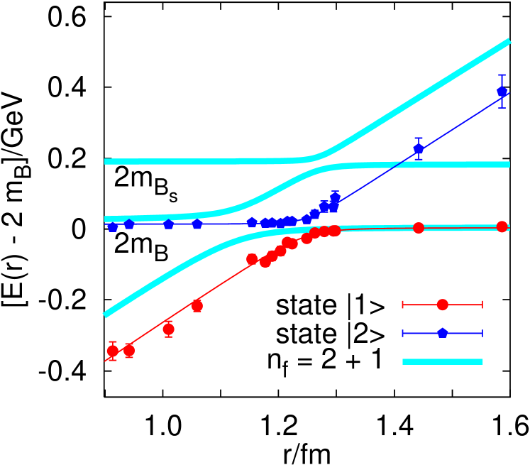
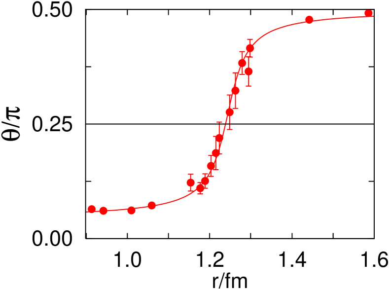
Figure 1: The energy levels and the mixing angle $\theta$ in physical units for $n_{f}=2$. The bands in the left figure reflect the expected $n_{f}=2+1$ scenario.

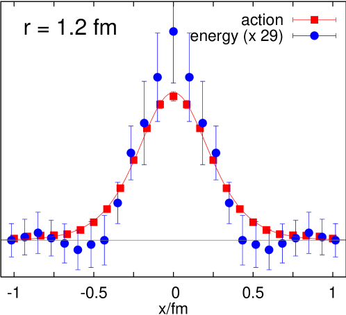
Figure 2: The transverse profile in the centre of the flux tube.

The quality of our density distribution data is depicted in Figure 2 for the ground state at a separation slightly smaller than $r_{c}$, as a function of the transverse distance $x$ from the $\overline{Q}Q$ axis. Due to cancellations between the magnetic and electric components the energy density is much smaller than the action density: for the comparison we have multiplied the energy density data by the arbitrary factor of 29. Note that the ratio $\sigma/\epsilon$ will diverge like $-\ln a\Lambda$ in the continuum limit. The differences between the shapes of the energy and action density distributions are not statistically significant. Here we only visualize the more precise action density results.

We employ several off-axis separations. Assuming rotational symmetry about the interquark axis, each point is labelled by two coordinates. $x$ denotes the distance from the $\overline{Q}Q$ axis and $y$ denotes the longitudinal distance from the centre point. We define an interpolating rectangular grid with perpendicular lattice spacing $a$ and the longitudinal spacing slightly scaled, such that the static sources always lie on integer grid coordinates. We then assign a quadratically interpolated value to each grid point ${\mathbf{z}}$, obtained from points in the neighbourhood, $|{\mathbf{z}}-(x,y)|\leq\epsilon=a$. On the axis the data points are more sparse and we relax the condition to $\epsilon=\sqrt{3}a$ while for the singular peaks we maintain the un-interpolated values.

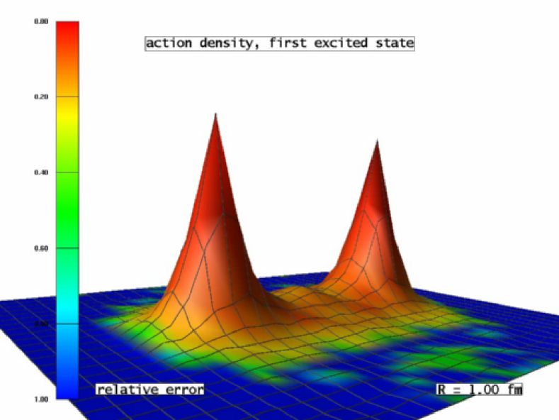
Figure 3: Action density distribution for the ground state and the first excitation.

We append two mpeg animations of the action density distribution as a function of the distance $1\,\mbox{fm}\leq r\leq 1.5$ fm for the ground state (string fission) and the excited state (string fusion). The picture frames inbetween the measurement points of Figure 1 are linearly interpolated. Note that the time is not a linear function of the distance but dilated within the string breaking region. On a linear time scale string breaking takes place rather rapidly. The starting frames are displayed in Fig. 3. The colour encodes the relative statistical errors and the lattice mesh represents our spatial resolution $a$. In spite of the fact that the excited state has (within errors) the energy of two isolated static-light mesons, a significant string component is already present at $r<r_{c}$ which then grows as $r$ is further increased. This is already obvious from the $\theta(r)$ of Figure 1.

4 Conclusion

At any distance the action density looks like a superposition between (hypothetical) $\overline{Q}Q$ and $B\overline{B}$ distributions with little interference: light pair creation seems to occur non-localized and instantaneously. Applying the decay model of Ref. [5], where the interaction term is instantaneous and only depends on the separation $r$, we undershoot the experimental $\Upsilon(4S)\rightarrow B\overline{B}$ decay rate by a factor of about two. This appears very reasonable, considering the crudeness of the model and the fact that the gap $\Delta E_{c}$ will increase with lighter, more realistic sea quark masses. We are studying the situation in more detail.

References

- [1] C. Michael, Hadronic decays, arXiv:hep-lat/0509023.
- [2] G.S. Bali et al., String breaking with dynamical Wilson fermions, arXiv:hep-lat/0409137.
- [3] G.S. Bali et al. [SESAM Collaboration], Observation of string breaking in QCD, Phys. Rev. D 71 (2005) 114513 [arXiv:hep-lat/0505012].
- [4] N. Brambilla, A. Pineda, J. Soto and A. Vairo, Effective field theories for heavy quarkonium, arXiv:hep-ph/0410047.
- [5] I.T. Drummond and R.R. Horgan, Lattice string breaking and heavy meson decays, Phys. Lett. B 447 (1999) 298 [arXiv:hep-lat/9811016].
- [6] G.S. Bali, K. Schilling and C. Schlichter, Observing long color flux tubes in SU(2) lattice gauge theory, Phys. Rev. D 51 (1995) 5165 [arXiv:hep-lat/9409005].