Nucleon Structure from Quenched Overlap Fermions

Abstract:

We compute the lowest moments of the nucleon’s structure functions using quenched overlap fermions at two different lattice spacings. The renormalisation is done nonperturbatively in the $\mathrm{RI^{\prime}-MOM}$-scheme.

PoS(LAT2005)363

1 INTRODUCTION

Information about the internal structure of the nucleon is encoded in its structure functions. While they cannot be computed directly on the lattice, the operator product expansion (OPE) provides a connection between their moments and nucleon matrix elements of local operators. For instance, for the unpolarised structure function $F_{1}$, the OPE reads

$$2\int_{0}^{1}{dxx^{n-1}F_{1}(x,Q^{2})=\sum_{f}E^{(f)}_{F_{1},n}v_{n}^{(f)}+O(1/Q^{2})},$$ (1)

where $f$ denotes the quark flavour, $E^{(f)}_{F_{1},n}$ is the (perturbative) Wilson coefficient and the matrix element $v_{n}^{(f)}$ is defined by

$$\langle N(\vec{p})|O_{(f)}^{\{\mu_{1}\ldots\mu_{n}\}}-\mathrm{traces}|N(\vec{p})\rangle=2v_{n}^{(f)}(p^{\mu_{1}}\ldots p^{\mu_{n}}-\mathrm{traces}),$$ (2)

with the operator

$$O_{(f)}^{\mu_{1}\ldots\mu_{n}}=\bar{\psi}_{f}\gamma^{\mu_{1}}\stackrel{{\scriptstyle\leftrightarrow}}{{D^{\mu_{2}}}}\ldots\stackrel{{\scriptstyle\leftrightarrow}}{{D^{\mu_{n}}}}\psi_{f}.$$ (3)

Similar relations hold for the other structure functions, see e.g. [1] for details. Both the matrix element $v_{n}^{(f)}$ and the Wilson coefficient $E^{(f)}_{F_{1},n}$ depend upon the choice of a renormalisation scheme and scale; only in their product, these dependencies cancel.

2 LATTICE SIMULATION

We use the overlap operator given by

$$D=\rho\big{(}1+\frac{m_{q}}{2\rho}+(1-\frac{m_{q}}{2\rho})\gamma_{5}\mbox{sgn}(H_{W}(-\rho))\big{)},$$ (4)

where $H_{W}(-\rho)=\gamma_{5}(D_{W}-\rho)$, $D_{W}$ being the Wilson Dirac operator. We approximate the sign function appearing in (4) by minmax polynomials [2]. For the gauge part we chose the Lüscher-Weisz action [3]

$$S[U]=\frac{6}{g^{2}}\left(c_{0}\sum_{\rm plaq}\mbox{\small$\frac{1}{3}$}\mbox{Re}\,\mbox{Tr}\,[1-U_{\rm plaq}]+c_{1}\sum_{\rm rect}\mbox{\small$\frac{1}{3}$}\mbox{Re}\,\mbox{Tr}\,[1-U_{\rm rect}]+c_{2}\sum_{\rm par}\mbox{\small$\frac{1}{3}$}\mbox{Re}\,\mbox{Tr}\,[1-U_{\rm par}]\right),$$ (5)

$V$ $\beta$ $a(\mbox{fm})$ confs. $16^{3}32$ $8.00$ $0.153(3)\mbox{fm}$ 300 $24^{3}48$ $8.45$ $0.105(2)\mbox{fm}$ 200

Table 1: Parameters of the gauge configurations used.

with coefficients $c_{1}$, $c_{2}$ ($c_{0}+8c_{1}+8c_{2}=1$) taken from tadpole improved perturbation theory [4]. We ran our computations at two lattice spacings, see table 1. The scale has been set from the pion decay constant, details are given in [5]. The parameter $\rho$ in (4) was set to $1.4$.

In order to remove $O(a)$ errors from the three-point functions, we employ the method of [6], which amounts to replacing propagators $D^{-1}\Psi$ by $\frac{1}{1-\frac{m}{2\rho}}D^{-1}\Psi-\frac{1}{2(1-\frac{m}{2\rho})}\Psi$. Jacobi smeared point sources [1] with parameters $N_{s}=50$ and $\kappa_{s}=0.21$ have been used in order to obtain a good overlap with the ground state.

The computation of matrix elements follows the procedure outlined in [1]: We form the ratio

$$R=\frac{\langle N(t_{sink})O(\tau)\bar{N}(t_{source})\rangle}{\langle N(t_{sink})\bar{N}(t_{source})\rangle},$$ (6)

from which the matrix element can be extracted in the region $t_{source}<\tau<t_{sink}$. We always set $t_{source}=0$ and $t_{sink}=9$ ($t_{sink}=13$) on the $\beta=8.0$ ($\beta=8.45$) configurations (in lattice units), which corresponds to a distance between source and sink of $1.4~{}\mbox{fm}$.

The matrix elements we are considering are listed in table 2, along with the operators used for their determination, where we use the operators (3) and

$$O_{5,(f)}^{\mu_{1}\ldots\mu_{n}}=\bar{\psi}_{f}\gamma_{5}\gamma^{\mu_{1}}\stackrel{{\scriptstyle\leftrightarrow}}{{D^{\mu_{2}}}}\ldots\stackrel{{\scriptstyle\leftrightarrow}}{{D^{\mu_{n}}}}\psi_{f}.$$ (7)

We compute only flavour non-singlet matrix elements, since in this case there is no contribution from disconnected diagrams.

Matrix Element Operator $g_{A}$ $\bar{\psi}\gamma^{5}\gamma^{2}\psi$ $g_{T}$ $\bar{\psi}\gamma^{5}\sigma^{24}\psi$ $v_{2}$ $O^{44}-\mbox{\small$\frac{1}{3}$}\left(O^{11}+O^{22}+O^{33}\right)$ $a_{1}$ $\mbox{\small$\frac{1}{2}$}\left(O_{5}^{24}+O_{5}^{42}\right)$

Table 2: Operators used in the three-point functions.

3 NON-PERTURBATIVE RENORMALISATION

The operators appearing inside the three-point functions have to be renormalised. For $g_{A}=\Delta u-\Delta d$, the operator to be used is the axial current $A_{\mu}$, the renormalisation of which is particularly simple because it does not depend on a renormalisation scheme or scale. It can be obtained from a Ward identity [7] as

$$Z_{A}=\lim_{m_{q}\rightarrow 0}\lim_{t\rightarrow\infty}\frac{2m_{q}}{m_{\pi}}\frac{\langle P(t)P(0)\rangle}{\langle A_{4}(t)P(0)\rangle}.$$ (8)

The renormalisation constants of the other operators under consideration are logarithmically divergent. We have computed them in the $\mathrm{RI^{\prime}-MOM}$-scheme [8]. In this scheme, the renormalisation condition is formulated in terms of quark Greens functions in Landau gauge with an operator insertion at zero momentum transfer:

$$C_{O}(p)=\frac{1}{V}\sum_{x,y,z}{e^{-ip(x-y)}\langle\psi(x)O(z)\bar{\psi}(y)\rangle}.$$ (9)

From this quantity, the amputated vertex function $\Gamma_{O}$ is formed:

$$\Gamma_{O}(p)=S^{-1}(p)C_{O}(p)S^{-1}(p),$$ (10)

with the quark propagator

$$S(p)=\frac{1}{V}\sum_{x,y}{e^{-ip(x-y)}\langle\psi(x)\bar{\psi}(y)\rangle}.$$ (11)

The renormalisation condition at scale $\mu$ is

$$\left.Z_{\psi}(\mu)Z_{O}(\mu)\Pi_{O}\left(\Gamma_{O}(p)\right)\right|_{p^{2}=\mu^{2}}=1,$$ (12)

with the projector $\Pi_{O}(\Gamma)=\mbox{\small$\frac{1}{12}$}\mbox{tr}\left(\Gamma_{O,\mathrm{Born}}^{-1}(p)\Gamma\right)$. The wavefunction renormalisation constant $Z_{\psi}$ has been determined from the relation $Z_{\psi}Z_{A}\Pi_{A}\left(\Gamma_{A}\right)=1$.

In order to convert the results to the $\overline{\mathrm{MS}}$-scheme, we first determine the renormalisation group invariant renormalisation constant $Z_{O}^{\mathrm{RGI}}$:

$$Z_{O}^{\mathrm{RGI}}=\left(Z_{O}^{\mathrm{RI^{\prime}-MOM},\mathrm{RGI}}(\mu)\right)^{-1}Z_{O}^{\mathrm{RI^{\prime}-MOM}}(\mu),$$ (13)

and then convert to the $\overline{\mathrm{MS}}$-scheme at scale $\mu^{\prime}$ (we always use $\mu^{\prime}=2\mbox{GeV}$):
$Z_{O}^{\overline{\mathrm{MS}}}(\mu^{\prime})=Z_{O}^{\overline{\mathrm{MS}},\mathrm{RGI}}(\mu)Z_{O}^{\mathrm{RGI}}$ with the conversion functions

$$Z^{{\cal S},\mathrm{RGI}}_{O}(\mu)=\left(2b_{1}{g^{\cal S}(\mu)}^{2}\right)^{-\frac{d_{O,1}}{2b_{1}}}\exp{\left[\int_{0}^{g^{\cal S}(\mu)}d\xi\left(\frac{\gamma^{S}_{O}(\xi)}{\beta^{S}(\xi)}+\frac{d_{O,1}}{b_{1}\xi}\right)\right]}.$$ (14)

The coefficients of the $\beta$ and $\gamma$ functions are taken from [9, 10].

In fig. 1 we plot $Z_{v_{2b}}^{\mathrm{RI^{\prime}-MOM}}$ and $Z_{v_{2b}}^{\mathrm{RGI}}$ for $\beta=8.45$. From the latter plot, we read off $Z_{v_{2b}}^{\mathrm{RGI}}=2.6$ from the plateau region $8\mbox{GeV}^{2}<p^{2}<15\mbox{GeV}^{2}$. Using $Z_{v_{2b}}^{\overline{\mathrm{MS}},\mathrm{RGI}}(2\mbox{GeV})=0.737$, we obtain $Z_{v_{2b}}^{\overline{\mathrm{MS}}}=1.92$. The renormalisation constants for all operators we need are shown in table 3. A comparison with results obtained in one-loop tadpole-improved lattice perturbation theory [11, 12] shows large discrepancies, especially for the operators with one derivative.

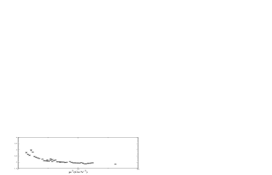
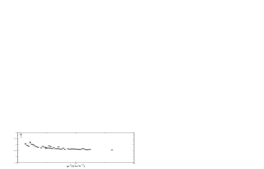
Figure 1: Left: The renormalisation constant $Z_{v_{2b}}^{\mathrm{RI^{\prime}-MOM}}(\mu)$, Right: The same, but with the renormalisation group running removed according to (13).

Operator $\beta=8.0$ $\beta=8.45$ pert. nonp. pert. nonp. $O_{A_{\mu}}$ 1.36 $1.59$ $1.30$ $1.42$ $O_{g_{T}}$ 1.36 $1.73$ $1.33$ $1.54$ $O_{v_{2}}$ 1.33 $2.11$ $1.39$ $1.92$ $O_{a_{1}}$ 1.34 $2.21$ $1.40$ $1.98$

Table 3: Comparison between the renormalisation constants $Z_{O}^{\overline{\mathrm{MS}}}(2\mbox{GeV})$ obtained non-perturbatively and in lattice perturbation theory.

4 RESULTS

Our results for the axial charge $g_{A}$ are displayed in fig. 2 (left). A linear extrapolation to the chiral limit yields $g_{A}=1.37(5)$ at $\beta=8.0$ and $g_{A}=1.14(5)$ at $\beta=8.45$. The tensor charge $g_{T}=\delta u-\delta d$ is plotted in fig. 2 (right); in this case, linear extrapolations to $m_{q}=0$ yield $g_{T}=1.35(4)$ at $\beta=8.0$ and $g_{T}=1.18(5)$ at $\beta=8.45$.

The results for the matrix elements $v_{2}^{u-d}=\langle x\rangle^{u-d}$ and $a_{1}^{u-d}=2\langle x\rangle^{\Delta u-\Delta d}$ are shown in fig. 3, together with the phenomenological values. In both cases, there is almost no dependence on the quark mass visible. In the range $m_{\pi}\gtrsim 400\mbox{MeV}$, our results agree with previous results obtained from improved Wilson fermions [1].

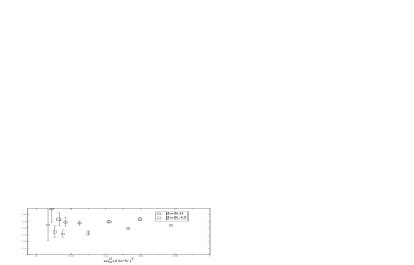
Figure 2: The nucleon’s axial charge (left plot) and tensor charge (right plot) as a function of the squared pion mass

Figure 3: The nucleon matrix elements $a_{1}^{u-d}$ (left plot) and $v_{2}^{u-d}$ (right plot) as functions of the squared pion mass ($\overline{\mathrm{MS}}$, $2\mbox{GeV}$).

5 CONCLUSIONS

We have determined the flavour non-singlet nucleon matrix elements $g_{A}$, $g_{T}$, $v_{2}$ and $a_{1}$ from quenched overlap fermions. The renormalisation has been done nonperturbatively. Comparing the results at the two values for the lattice spacing we have, we find significant discretisation effects, in contrast with the situation for hadron masses [5].

While our results are in good agreement with earlier determinations, there remains a rather large discrepancy to the phenomenological values for $v_{2}$ and $a_{1}$, even at the lowest quark masses we can reach at present.

References

[1]
M. Göckeler, R. Horsley, E.-M. Ilgenfritz, P. Rakow, G. Schierholz,
A. Schiller, Phys. Rev. D53 (1996) 2317.
[2]
L. Giusti, M. Lüscher, P. Weisz, H. Wittig,
Comp. Phys. Comm. 153 (2003) 31.
[3]
M. Lüscher, P. Weisz, Comm. Math. Phys. 97 (1985) 59.
[4]
C. Gattringer, R. Hoffmann, S. Schaefer, Phys. Rev. D65 (2002) 094503.
[5]
M. Gürtler et al., PoS (LAT2005) 077.
[6]
S. Capitani, M. Göckeler, R. Horsley, P.E.L. Rakow, H. Perlt, G. Schierholz,
A. Schiller, Phys. Lett. B468 (1999) 150.
[7]
L. Giusti, C. Hoelbling, C. Rebbi,
Nucl. Phys. Proc. Suppl. 106 (2002) 739.
[8]
G. Martinelli, C. Pittori, C. T. Sachrajda, M. Testa and A. Vladikas,
Nucl. Phys. B 445 (1995) 81.
[9]
J. A. Gracey,
Nucl. Phys. B 662 (2003) 247.
[10]
J. A. Gracey,
Nucl. Phys. B 667 (2003) 242.
[11]
R. Horsley, H. Perlt, P. E. L. Rakow, G. Schierholz and A. Schiller [QCDSF
Collaboration],
Nucl. Phys. B 693 (2004) 3
[Erratum-ibid. B 713 (2005) 601].
[12]
R. Horsley, H. Perlt, P. E. L. Rakow, G. Schierholz and A. Schiller [QCDSF
Collaboration],
arXiv:hep-lat/0505015.