DESY/05-195 HU-EP-05/45 October 2005
Scaling test of fermion actions
in the Schwinger model

We discuss the scaling behaviour of different fermion actions in dynamical simulations of the 2-dimensional massive Schwinger model. We have chosen Wilson, hypercube, twisted mass and overlap fermion actions. As physical observables, the pion mass and the scalar condensate are computed for the above mentioned actions at a number of coupling values and fermion masses. We also discuss possibilities to simulate overlap fermions dynamically avoiding problems with low-lying eigenvalues of the overlap kernel.

1 Introduction

Besides the interest in the 2-dimensional Schwinger model [1] in its own right as a quantum field theory, it can be considered as a test laboratory for new theoretical concepts and ideas that aim at eventual applications in more demanding situations such as lattice QCD. In particular, for numerical simulations the lattice Schwinger model is most suitable to perform test studies since the computations are much cheaper than in four dimensions and precise results at many parameter values can be obtained, see e.g. refs. [2, 3, 4, 5] for a selection of recent work in the Schwinger model. In this paper, we want to address the scaling properties of a number of fermion actions for $N_{f}=2$ flavours of dynamical fermions. To this end, we will compare standard Wilson [6], Wilson twisted mass [7, 8], hypercube [9] and overlap fermions [10] in their approach to the continuum limit. We will use throughout the paper the Wilson plaquette gauge action with a coupling $\beta=1/a^{2}e^{2}$, with $a$ the lattice spacing and $e$ the dimensionful coupling.

Each of the above mentioned fermion actions has certain advantages and are used in present simulations of lattice QCD. Understanding the scaling properties when using different lattice actions and to check the expected scaling behaviour as a function of the lattice spacing $a$ is certainly one of the most important questions in lattice calculations. However, if we think of dynamical fermion simulations in lattice QCD a scaling analysis is, at least nowadays, far too computer time consuming to be addressed, see e.g. ref. [11] and ref. [12] for recent estimates of the simulation costs in lattice QCD. On the other hand, for the 2-dimensional Schwinger model, such simulations are perfectly possible and give important insight into the properties of the above mentioned actions.

In order to study the scaling behaviour, we will fix the scaling variable $z\equiv(m_{f}\sqrt{\beta})^{2/3}$, where $m_{f}$ is the fermion mass in lattice units. We have chosen $z=0.2,0.4,0.8$. The fermion mass is determined from the PCAC relation where we employ local as well as conserved currents. At each of these fixed values of $z$ we compute the pseudo scalar mass and the scalar condensate and follow its behaviour with decreasing value of the lattice spacing. Performing finally a continuum limit of our results allows us to compare to analytical predictions that are available from approximations of the massive Schwinger model which cannot be solved exactly.

The paper is organized as follows. In section 2 we give the definition of the Wilson, hypercube, maximally twisted mass and overlap fermion operators which we have employed in this work. Section 3 is devoted to the observables we have used and provides a description of the numerical simulations, in particular our attempts to simulate overlap fermions dynamically. Section 4 contains our results and section 5 the conclusions.

2 Lattice fermions

In this section we give the definitions of the different kind of fermions we have used, i.e. Wilson, hypercube, Wilson twisted mass and overlap fermions. Throughout the work we have employed only the Wilson plaquette gauge action with gauge fields $U_{n,\mu}\in U(1)$, $n$ denoting a lattice point and $\mu=1,2$ a direction of the 2-dimensional lattice

$$S_{G}[U]=\beta\sum_{P}\frac{1}{2}\big{(}U_{P}+U_{P}^{\dagger}\big{)}$$ (1)

with $U_{P}$ denoting the plaquette

$$U_{P}=U_{n,1}U_{n+\hat{1},2}U^{\dagger}_{n+\hat{2},1}U^{\dagger}_{n,2}\;,$$ (2)

where $\hat{1}$ and $\hat{2}$ denote shifts in direction $1$ or $2$ respectively. The coupling multiplying the plaquette gauge action is $\beta=1/g^{2}$. Denoting by $e$ the physical coupling, dimensions are introduced by $\beta=1/a^{2}e^{2}$. We restrict ourselves to $N_{f}=2$ flavours of dynamical fermions.

2.1 Wilson fermions

As a first action that can serve as a kind of benchmark action, we have chosen standard Wilson fermions [6] with the Wilson operator $D_{\mathrm{W}}$ given by

$$D_{\mathrm{W}}^{n,m}=(m_{0}+2r)\delta_{n,m}-\frac{1}{2}\sum_{\mu}[(r-\sigma_{\mu})U_{n,\mu}\delta_{n,m-\hat{\mu}}+(r+\sigma_{\mu})U^{\dagger}_{m,\mu}\delta_{n,m+\hat{\mu}}]\;.$$ (3)

Here the sum goes over the two directions $\mu=1$ and $\mu=2$ and we use the standard Pauli-matrices $\sigma_{\mu},\mu=1,2,3$ with $\sigma_{3}=\mathrm{diag}(1,-1)$, $n,m$ denote lattice points with space and time coordinates $(x,t)$ and we suppress the Dirac indices. The Wilson parameter $r$ is chosen to be $r=1$ throughout the paper. The Wilson action is expected to lead to large discretization errors in physical observables linear in the lattice spacing $a$ and hence approaches the continuum limit rather slowly. We will compare results obtained with the Wilson action to corresponding results from actions where these $O(a)$ lattice artefacts are expected to vanish and changed to an $O(a^{2})$ behaviour.

2.2 Hypercube fermions

Perfect actions [9] are completely free of lattice artefacts. However, since such actions cannot be realized in practice, truncated versions are used which are expected to inherit many of the properties of the perfect actions. For this work, we have chosen a particular ansatz, the hypercube action [13]. In this approach the interaction among fields on the lattice is extended from a purely nearest neighbour interaction to a hypercube of the lattice.

A general ansatz for the hypercube operator is

$$D^{n,m}_{\mathrm{hyp}}=\sum_{\mu}\rho^{\mu}_{m-n}\sigma_{\mu}+\lambda_{m-n}\mathbbm{1},$$ (4)

where $\rho^{\mu}_{m-n}$ and $\lambda_{m-n}$ are real parameters, the values of which have to be optimized according to some criterion, e.g. by demanding an improved continuum limit behaviour of physical observables.

Furthermore, symmetry requirements of the action leads, in the case of the Schwinger model, to a reduction of these couplings to only 5 free parameters that will depend on the gauge coupling constant $g$ and the bare fermion mass $m_{\mathrm{hyp}}$. The values of $\rho$ and $\lambda$ are determined for free fermions, setting $g=0$ and then they are taken over to the interacting case. As an alternative, the values of $\rho$ and $\lambda$ may be determined by requiring that the violations of the Ginsparg-Wilson relation are minimized. In this work we will, however, only work with the “scaling optimized” set of parameters as given in ref. [14] since we are interested mainly in the scaling behaviour. We give in the following table the values of the parameters that we have used in this work.

$\lambda_{0}$	$+1.5+m_{\mathrm{hyp}}$
$\lambda_{1}$	$-0.25$
$\lambda_{2}$	$-0.125$
$\rho^{(1)}$	$+0.334$
$\rho^{(1)}$	$+0.083$

The full hypercube Dirac operator is given by

$$D_{\mathrm{hyp}} = \lambda_{0}+H^{(1)}+H^{(2)}\qquad$$

$$(H^{(1)})^{nm} = \sum_{\mu=1}^{2}\Big{(}U_{n,\mu}\delta_{n,m-\hat{\mu}}(\lambda_{1}+\sigma_{\mu}\rho^{(1)})+U^{\dagger}_{n-\hat{\mu},\mu}\delta_{n,m+\hat{\mu}}(\lambda_{1}-\sigma_{\mu}\rho^{(1)})\Big{)}$$

$$(H^{(2)})^{nm} = \frac{1}{2}\Big{(}(U_{n,1}U_{n+\hat{1},2}+U_{n,2}U_{n+\hat{2},1})\,\delta_{n,m-\hat{1}-\hat{2}}(\lambda_{2}+(\sigma_{1}+\sigma_{2})\rho^{(2)})$$

$$\ \ +(U_{n,1}U^{\dagger}_{n+\hat{1}-\hat{2},2}+U^{\dagger}_{n-\hat{2},2}U_{n-\hat{2},1})\,\delta_{n,m-\hat{1}+\hat{2}}(\lambda_{2}+(\sigma_{1}-\sigma_{2})\rho^{(2)})$$

$$\ \ +(U^{\dagger}_{n-\hat{1},1}U_{n-\hat{1},2}+U_{n,2}U^{\dagger}_{n+\hat{2}-\hat{1},1})\,\delta_{n,m+\hat{1}-\hat{2}}(\lambda_{2}+(-\sigma_{1}+\sigma_{2})\rho^{(2)})$$

$$\ \ +(U^{\dagger}_{n-\hat{1},1}U^{\dagger}_{n-\hat{1}-\hat{2},2}+U^{\dagger}_{n-\hat{2},2}U^{\dagger}_{n-\hat{1}-\hat{2},1})\,\delta_{n,m+\hat{1}+\hat{2}}(\lambda_{2}+(-\sigma_{1}-\sigma_{2})\rho^{(2)})\Big{)}\;.$$

2.3 Twisted mass fermions

The twisted mass formulation of lattice fermions has been introduced originally to regulate small, unphysical eigenvalues of the Wilson lattice Dirac operator [7]. In order to keep an $O(a)$ improvement, the twisted mass setup has been first developed in the $O(a)$ Symanzik improved theory. However, it then was realized that by a careful tuning of the parameters of the Wilson twisted mass action, an automatic, full $O(a)$-improvement can be reached, leading to lattice discretization errors that appear only in $O(a^{2})$ and hence allow for a much accelerated continuum limit [8]. The Wilson twisted mass formulation has received a lot of attention recently and a number of tests in the quenched [15, 16, 17, 18, 19] and partly also for full dynamical fermions [20, 21, 22, 23] has been performed.

In order to introduce twisted mass fermions, let us start with the continuum, Euclidean action,

$$S[\bar{\psi},\psi]=\int d^{2}x\bar{\psi}(\sigma_{\mu}D_{\mu}+m+i\mu_{f}\sigma_{5}\tau_{3})\psi,$$ (6)

where $\tau_{3}$ is the third Pauli matrix, acting in flavour space and $\mu_{f}$ represents the twisted mass parameter. The transformation

$$\psi^{\prime}=e^{i\omega\sigma_{5}\frac{\tau_{3}}{2}}\psi$$

$$\bar{\psi}^{\prime}=\bar{\psi}e^{i\omega\sigma_{5}\frac{\tau_{3}}{2}}$$ (7)

leaves this form of the action invariant with rotated mass parameters,

$$m^{\prime} = m\cos\omega+\mu_{f}\sin\omega$$

$$\mu_{f}^{\prime} =- m\sin\omega+\mu_{f}\cos\omega\;,$$ (8)

with the rotation (“twist”) angle $\omega$,

$$\tan\omega=\frac{\mu_{f}}{m}\;.$$ (9)

On the lattice, the Wilson term is not invariant under the rotation in eq. (2.3) and the twisted mass operator takes the form

$$D_{\mathrm{tm}}=D_{\mathrm{W}}^{0}+\big{[}m_{0}+i\mu_{f}\sigma_{5}\tau_{3}\big{]}$$ (10)

where $D^{0}_{\mathrm{W}}$ denotes the Wilson operator without the mass term, i.e.

$$D_{\mathrm{W}}^{0}=D_{\mathrm{W}}[m_{0}=0]\;.$$ (11)

It can be shown that the twisted mass action leads to an O(a)-improvement when the angle $\omega=\pi/2$. It goes beyond the scope of this paper to provide the arguments for this remarkable result the derivation of which can be found in ref. [8]. We only would like to remark that in order to obtain this value of the twist angle is equivalent to tune the bare fermion mass parameter $m_{0}$ to a critical value $m_{0}^{\mathrm{crit}}$.

One very important aspect of twisted mass fermions is that there is a particular definition of $m_{0}^{\mathrm{crit}}$ from the vanishing of the PCAC fermion mass that does not only lead to an $O(a)$-improvement [24, 25, 16, 8, 17] but also substantially reduces cut-off effects that appear in $O(a^{2})$ as has been demonstrated in [26, 18]. In this paper, we will use a value of $m_{0}^{\mathrm{crit}}$ that was obtained in the pure Wilson fermion theory without twisted mass term from the PCAC relation. The value of $m_{0}^{\mathrm{crit}}$ was then tuned in such a way that the corresponding PCAC fermion mass vanishes. After having determined $m_{0}^{\mathrm{crit}}$ in this way, we varied the twisted mass parameter $\mu_{f}$ to realize the fermion and pion masses we are interested in.

2.4 Overlap fermions

A lattice Dirac operator $D_{\rm GW}$ that satisfies the Ginsparg-Wilson relation [27]

$$D_{\rm GW}\gamma_{5}+\gamma_{5}D_{\rm GW}=2aD_{\rm GW}\gamma_{5}RD_{\rm GW}\ ,$$ (12)

where $R$ is a local term, leads to an action that has an exact (lattice) chiral symmetry eliminating thus automatically $O(a)$ cut-off effects. The realization of an operator $D_{\rm GW}$ that we use here is the overlap fermion, which is characterized by the overlap Dirac operator [10]. For $R_{n,m}=\frac{\delta_{n,m}}{2\rho}$ it takes the form

$$D_{\rm ov} = \Big{(}1-\frac{m_{\rm ov}\bar{a}}{2}\Big{)}D_{\rm ov}^{(0)}+m_{\rm ov}\ ,$$ (13)

$$D_{\rm ov}^{(0)} = \frac{1}{\bar{a}}\left\{1+D_{0}/\sqrt{D_{0}^{\dagger}D_{0}}\right\}$$ (14)

where $D_{0}$ is the so-called overlap kernel operator and $\bar{a}\equiv a/\rho$. For the kernel $D_{0}$, there is a large choice. In the following, however, we will only use the hypercube operator, i.e. $D_{0}=D_{\mathrm{hyp}}$ with fixed $\lambda_{0}=0.5$, i.e. setting $m_{\mathrm{hyp}}=-1$. This corresponds to setting the parameter $\rho=1$ in eq. (14) and guarantees the locality of the overlap operator [28].

We remark that we have realized the square root operator $1/\sqrt{D_{0}^{\dagger}D_{0}}$ in eq. (14) by Chebyshev polynomials $P_{n,\epsilon}$ with degree $n$ and a lower bound $\epsilon$. This Chebyshev polynomial shows an exponential convergence rate in the interval $[\epsilon,1]$. Setting $\epsilon$ to the lowest eigenvalue of the overlap kernel operator $D_{0}^{\dagger}D_{0}$ which is normalized to one, we always have chosen the degree $n$ such that we reach machine precision for the evaluation of $1/\sqrt{D_{0}^{\dagger}D_{0}}$. We used eigenvalue deflation and projected out a number of low-lying eigenvalues. In this case, $\epsilon$ was set to the lowest non-projected eigenvalue of $D_{0}^{\dagger}D_{0}$.

3 Observables and simulations

In this section we give the operators that we have used to determine the physical observables we have computed and describe the numerical simulations. In particular, we discuss some of our attempts to perform dynamical overlap simulations avoiding problems with very low-lying eigenvalues of the overlap kernel operator.

3.1 Observables

2-point functions

Generally, the bi-linear operators are given by

$$\mathcal{\tilde{O}}_{n}^{\Gamma\tau}=\bar{\psi}_{n}\Gamma\tau\psi_{n},$$ (15)

where $\Gamma$ stands for certain combinations of the Pauli matrices $\sigma$ acting in Dirac-space, while the Pauli matrices $\tau$ act in flavour space. We will consider the following operators,

$$\mathcal{\tilde{P}}^{a}_{n} = \bar{\psi}_{n}\sigma^{(Dirac)}_{3}\tau_{a}^{(flavour)}\psi_{n}$$ (16)

$$\mathcal{\tilde{S}}_{n} = \bar{\psi}_{n}\psi_{n}$$ (17)

$$\mathcal{\tilde{A}}^{\mu a}_{n} = \bar{\psi}_{n}\sigma^{(Dirac)}_{3}\sigma^{(Dirac)}_{\mu}\tau_{a}^{(flavour)}\psi_{n}$$ (18)

$$\mathcal{\tilde{V}}^{\mu a}_{n} = \bar{\psi}_{n}\sigma^{(Dirac)}_{\mu}\tau_{a}^{(flavour)}\psi_{n},$$ (19)

with $\mathcal{\tilde{P}}$ the pseudo scalar, $\mathcal{\tilde{S}}$ the scalar, $\mathcal{\tilde{A}}$ the axial-vector and $\mathcal{\tilde{V}}$ the vector operator.

For the twisted mass fermions, the operators take a modified form as can be obtained from the field transformation according to eq. (2.3), leading to

$$\mathcal{\tilde{P}}^{a(ph)}_{n} = \left\{\begin{array}[]{ll}\mathcal{\tilde{P}}^{a(tb)}_{n}&\textrm{if}\ a=1,2\\ \cos\omega\,\mathcal{\tilde{P}}^{3(tb)}_{n}+\sin\omega\,\mathcal{\tilde{S}}_{n}^{(tb)}&\textrm{if}\ a=3\end{array}\right.$$ (22)

$$\mathcal{\tilde{A}}^{\mu a(ph)}_{n} = \left\{\begin{array}[]{ll}\cos\omega\,\mathcal{\tilde{A}}^{\mu a(tb)}_{n}+\sin\omega\,\epsilon_{ab}\mathcal{\tilde{V}}^{\mu b(tb)}_{n}&\textrm{if}\ a=1,2\\ \mathcal{\tilde{A}}^{\mu 3(tb)}_{n}&\textrm{if}\ a=3\end{array}\right.$$ (25)

$$\mathcal{\tilde{V}}^{\mu a(ph)}_{n} = \left\{\begin{array}[]{ll}\cos\omega\,\mathcal{\tilde{V}}^{\mu a(tb)}_{n}+\sin\omega\,\epsilon_{ab}\mathcal{\tilde{A}}^{\mu b(tb)}_{n}&\textrm{if}\ a=1,2\\ \mathcal{\tilde{V}}^{\mu 3(ph)}_{n}.&\textrm{if}\ a=3\end{array}\right.$$ (28)

Here “ph” denotes the physical and “tb” the twisted basis. Note that in the special case $\omega=\pi/2$ for $a=1,2$, $\mathcal{\tilde{V}}$ and $\mathcal{\tilde{A}}$ just interchange their role while $\mathcal{\tilde{P}}$ remains invariant. In particular, the scalar operator is given by the 3rd component of the pseudo scalar operator.

For the Wilson, hypercube and Wilson twisted mass fermions we computed the 2-point correlation functions by standard techniques using a conjugate gradient solver. For overlap fermions we calculated the correlators both from using a conjugate gradient solver and from eigenvectors $\phi_{i}$ and eigenvalues $\lambda_{i}$ of the overlap operator in eq. (13). A generic non-singlet correlator $C(n,m)$ is then expressed in terms of the fermion propagator $S(n,m)$ and a suitable Dirac structure $\Gamma$, corresponding to the operators listed above, as

$$C(n,m) = tr[\Gamma S(n,m)\Gamma S(m,n)]$$ (29)

$$= \sum_{\lambda_{i},\lambda_{j}}\frac{1}{\lambda_{i}\lambda_{j}}\sum_{\alpha\beta\gamma\delta}\bigg{[}(\phi^{{\dagger}\alpha}_{j}(n)\Gamma_{\alpha\beta}\phi^{\beta}_{i}(n))(\phi^{{\dagger}\gamma}_{i}(m)\Gamma_{\gamma\delta}\phi^{\delta}_{j}(m))\bigg{]}\;.$$

PCAC fermion mass

The bare mass parameter for Wilson ($m_{0}$) and hypercube ($m_{\mathrm{hyp}}$) fermions receives an additive mass renormalization, necessitating the determination of a critical fermion mass $m_{\mathrm{crit}}$ which we computed by the vanishing of the PCAC fermion mass, extracted from the PCAC relation

$$\langle\partial_{\mu}\mathcal{\tilde{A}}^{\mu}(n)\mathcal{\tilde{O}}\rangle=2m\langle\mathcal{\tilde{P}}(n)\mathcal{\tilde{O}}\rangle.$$ (30)

Choosing $\mathcal{\tilde{O}}=\mathcal{\tilde{P}}$ and projecting to zero momentum (denoting by $\mathcal{A}$ and $\mathcal{P}$ the currents summed over space), we arrive at

$$m_{f}(t)=\frac{\langle\partial_{2}\mathcal{A}^{2}_{t}\mathcal{P}_{0}\rangle}{2\langle\mathcal{P}_{t}\mathcal{P}_{0}\rangle}.$$ (31)

For the currents that appear in eq. (31) one may use the local currents of eqs. (16-19). An alternative is to employ also conserved currents. A very general way to derive the conserved currents is given in [29]. The vector and axial currents are then given by

$$\mathcal{\tilde{V}}^{\mu a}_{n} = \tilde{J}^{\mu R}_{n}+\tilde{J}^{\mu L}_{n}$$ (32)

$$\mathcal{\tilde{A}}^{\mu a}_{n} = \tilde{J}^{\mu R}_{n}-\tilde{J}^{\mu L}_{n}$$ (33)

where

$$\tilde{J}^{\mu R}_{n}=\frac{1}{2}\bar{\psi}(1-\sigma_{3})\mathcal{K}^{\mu,n}(1+\sigma_{3})\psi$$ (34)

$$\tilde{J}^{\mu L}_{n}=\frac{1}{2}\bar{\psi}(1+\sigma_{3})\mathcal{K}^{\mu,n}(1-\sigma_{3})\psi$$ (35)

and

$$\mathcal{K}^{\mu,n}=-i\frac{\delta D(U^{(\alpha)})}{\delta\alpha_{n,\mu}}\Big{|}_{\alpha=0}\;,\;\;\qquad U^{(\alpha)}_{n,\mu}=e^{i\alpha_{n,\mu}}U_{n,\mu}$$ (36)

where $D(U^{(\alpha)}_{\mu})$ denotes the lattice Dirac operator used. This method of constructing the conserved currents is very useful when complicated lattice Dirac operators are considered since their construction from the current conservation condition can be very cumbersome. We followed this prescription to compute the conserved currents, only for the overlap fermions we used the local point currents. We remark that for the twisted mass and the overlap case in principle also the bare fermion masses, $\mu_{f}$ and $m_{\mathrm{ov}}$ can be used. However, since this could lead to very different lattice artefacts, we employed also in these cases the fermion mass derived from the PCAC relation for all physical results presented in the following in order to be able to directly compare the different fermion actions.

Scalar condensate

Besides the 2-point functions which will provide the pseudo scalar mass, we considered also the scalar condensate, $\Sigma\equiv\langle\bar{\psi}\psi\rangle$. A first method to compute $\Sigma$ is by calculating $\mathrm{Tr}D^{-1}$ using Gaussian noise sources. We will denote the so computed values of $\Sigma$ as $\Sigma_{\mathrm{direct}}$. This quantity develops in the case of Wilson and hypercube fermions a divergent piece $\propto 1/a$. A second way, which avoids the appearance of the divergent piece from the beginning, is to use the integrated axial Ward identity leading to a “subtracted” scalar condensate, $\Sigma_{\mathrm{sub}}$ [30]. We remark that in the case of overlap fermions we computed $\Sigma$ from the improved scalar operator $\langle\bar{\psi}(1-\frac{a}{2}D)\psi\rangle$ which we evaluated from the the eigenvalues of the overlap operator. More precise definitions and a further discussion will be provided in section 4.

3.2 Simulations

In our work, we have used for the Wilson, the hypercube and the twisted mass fermion action a standard Hybrid Monte Carlo algorithm (HMC) [31]. In the case of overlap fermions a straightforward implementation of the HMC algorithm is not suitable since the variation of the Hamiltonian with respect to the gauge field can lead to very large forces proportional to $(D_{0}^{\dagger}D_{0})^{-3/2}$ when the overlap kernel operator $D_{0}$ develops exceptionally small eigenvalues. See refs. [32, 33, 34] for variants of the HMC algorithm that circumvent this difficulty.

For the overlap fermion results we used configurations that were generated in the pure gauge theory only and performed a reweighting with the overlap fermion determinant to obtain physical observables for dynamical $N_{f}=2$ flavours of fermions. However, we also tried several possibilities to avoid the problem with low-lying eigenvalues of the overlap kernel operator $D_{0}$ by replacing $D_{\mathrm{ov}}$ by some operator $D_{\mathrm{ov}}^{\mathrm{approx}}$ that is a good approximation to $D_{\mathrm{ov}}$ but which is safe against these low-lying eigenvalues. The simulation can then be made exact again by adding a correction step employing the ratio $D_{\mathrm{ov}}/D_{\mathrm{ov}}^{\mathrm{approx}}$.

The general idea is to write (we use for simplicity only a single operator here, in practice one would have to use the operator $D^{\dagger}D$, of course)

$$\mathrm{det}D_{\mathrm{ov}}=\mathrm{det}D_{\mathrm{ov}}^{\mathrm{approx}}\cdot\mathrm{det}\left[\frac{D_{\mathrm{ov}}}{D_{\mathrm{ov}}^{\mathrm{approx}}}\right]\equiv\mathrm{det}D_{\mathrm{ov}}^{\mathrm{approx}}\cdot{R_{\mathrm{det}}}\;.$$ (37)

While $\mathrm{det}D_{\mathrm{ov}}^{\mathrm{approx}}$ would be used in the HMC algorithm, the remaining determinant ratio ${R_{\mathrm{det}}}$ could be implemented either in an additional accept/reject step or it could be included as a reweighting factor in the computation of a given observable.

A crucial question in such an approach is, whether an operator $D_{\mathrm{ov}}^{\mathrm{approx}}$ can be found such that the fluctuations in ${R_{\mathrm{det}}}$ are small enough to obtain statistically significant results. We decided therefore to test this idea by computing ${R_{\mathrm{det}}}$ stochastically using $n=10$ Gaussian noise vectors on a number of gauge field configurations generated in the pure gauge theory at $\beta=3$ on a $16^{2}$ lattice. In the following we will describe the results of these tests for three choices of $D_{\mathrm{ov}}^{\mathrm{approx}}$.

Case of $D_{\mathrm{ov}}^{\mathrm{approx}}=D_{\mathrm{hyp}}$

As a first trial, we used the hypercube operator $D_{\mathrm{hyp}}$ as an approximation to $D_{\mathrm{ov}}$. This choice has been motivated by the fact that the operator $D_{\mathrm{hyp}}$ is constructed to be approximating the Ginsparg-Wilson relation, resulting in a very similiar eigenvalue spectrum for both operators [14]. Note also that we have used the hypercube operator itself as an overlap kernel operator $D_{0}$. Let us remark that we re-write the massive overlap operator as $D_{\mathrm{ov}}^{(0)}+m_{\mathrm{ov}}/(1-m_{\mathrm{ov}}/2)$ in order to better match the eigenvalue spectra of both operators.

We computed ${R_{\mathrm{det}}}$ as a function of the hypercube bare fermion mass $m_{\mathrm{hyp}}$ in a range $-0.25<m_{\mathrm{hyp}}<0.25$. However, we found that the fluctuations of ${R_{\mathrm{det}}}$ were extremely large for all values of $m_{\mathrm{hyp}}$ we have tested. Thus we had to conclude that $D_{\mathrm{hyp}}$ cannot serve as an infrared safe, approximate operator for the overlap simulations when $R_{\mathrm{det}}$ is used in a stochastic correction step. We cannot exclude, of course, that by using an improved hypercube operator, e.g. by adding the clover term or performing smearing of the link variables, the situation could be improved. However, given the negative findings of our investigation, we did not pursue this direction. What we tried instead, is to use $D_{\mathrm{hyp}}$ as the guidance Hamiltonian in the molecular dynamics part of the Hybrid Monte Carlo algorithm while keeping $D_{\mathrm{ov}}$ as the exact overlap operator for the accept/reject Hamiltonian. Amazingly, despite the negative results described here for $R_{\mathrm{det}}$, we found that this led to reasonable acceptance rates, at least for not too large systems, see ref. [35] for a further discussion of this point.

Modified Chebyshev polynomial

As a second attempt, we tried to modify the range of the Chebyshev polynomial employed in the construction of the overlap operator. There, the square root of the kernel is computed by a Chebyshev polynomial $P_{n,\epsilon}$ of degree $n$ in the interval $\left[\epsilon,1\right]$,

$$P_{n,\epsilon}(D_{0}^{\dagger}D_{0})\approx 1/\sqrt{D_{0}^{\dagger}D_{0}}\;.$$ (38)

We have chosen the approximation accuracy in eq. (38) to be very high, compatible with machine (64-bit) precision. The value of $\epsilon$ is chosen to correspond to the lowest eigenvalue of $D_{0}^{\dagger}D_{0}$. In principle, it is possible to use instead of the “exact” polynomial with parameters $n$ and $\epsilon$ a modified polynomial with parameters ${\tilde{n}}<n$ and $\tilde{\epsilon}>\epsilon$. Clearly, if $\tilde{\epsilon}$ could be chosen to be well above the smallest eigenvalues of $D_{0}^{\dagger}D_{0}$ then using an overlap operator with a polynomial $P_{{\tilde{n}},\tilde{\epsilon}}$ in the molecular dynamics part would lead to an infrared safe simulation.

As a start situation, we had chosen $\tilde{\epsilon}=\epsilon$ and reduced only the degree of the polynomial successively. We found that it is indeed possible to reduce $n$ substantially to ${\tilde{n}}\approx 1/3\cdot n$ without having large fluctuations in the determinant ratio ${R_{\mathrm{det}}}$. This is a very positive outcome since it gives rise to a substantial acceleration of simulations with the overlap operator. However, when we tried to change the value of $\tilde{\epsilon}$ only slightly, we observed immediately large fluctuations in ${R_{\mathrm{det}}}$. For $\tilde{\epsilon}=1.1\cdot\epsilon$ the fluctuations in ${R_{\mathrm{det}}}$ became already so large that there is no chance to obtain a statistically significant result in such a setup.

Explicit infrared regularization

As a third (and last) attempt, we tried to use an approximate overlap operator that has an infrared regulator built in. In particular, we studied the situation where we use a modified sign function

$$D_{0}/\sqrt{D_{0}^{\dagger}D_{0}}\rightarrow D_{0}/(\sqrt{D_{0}^{\dagger}D_{0}+\delta)}\;.$$ (39)

The (optimistic) expectation here is that by choosing $\delta$ large enough, without having too large fluctuations in the determinant ratio ${R_{\mathrm{det}}}$, the overlap operator with such a modified sign function would be infrared safe for the HMC simulation.

Such an optimistic expectation is not completely unfounded when one inspects the eigenvalues of the exact overlap operator $D_{\mathrm{ov}}$ and the sign function modified one, $D_{\mathrm{ov}}^{\mathrm{approx}}$. Indeed, we show in fig. 1 the eigenvalues when choosing $\delta=0,0.0001,0.001,0.01$ for a typical configuration.

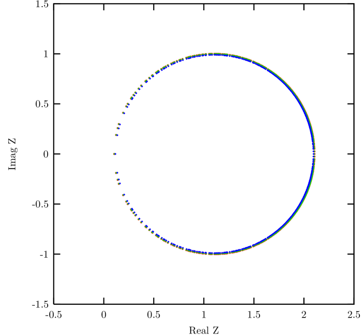
Figure 1: The eigenvalues of the exact overlap operator and a modified overlap operator when the sign function is changed according to eq. (39). The plot contains the eigenvalues for $\delta=0$ (the original overlap operator) and for $\delta=0.0001,0.001,0.01$. For all these cases, the eigenvalues are so close to each other that they cannot be distinguished in the graph.

As can be seen, all the eigenvalues lie on the expected circle and a difference for various choices of $\delta$ is not visible. In fig. 2 we show the difference of the eigenvalues between the spectra using $\delta=0$ and $\delta\neq 0$. In building the difference of the eigenvalues we used an ordering of the eigenvalues with respect to their real part. The scale in the plot is chosen for the situation of $\delta=0.01$. We have rescaled the difference in the eigenvalues by a factor of $30$ for $\delta=0.0001$ and $7$ for $\delta=0.001$ in order to plot all difference spectra in one common plot. It appears that the difference spectra do not build a perfect circle shape but are rather lemon shaped. Nevertheless the lemon distortion of the circle happens at a rather small scale of $O(10^{-2})$ for the case of $\delta=0.01$ while for smaller values of $\delta$ the difference becomes even smaller. Note that the smallest eigenvalue is $\lambda_{\mathrm{min}}(D_{0}^{\dagger}D_{0})=0.24$ for this configuration.

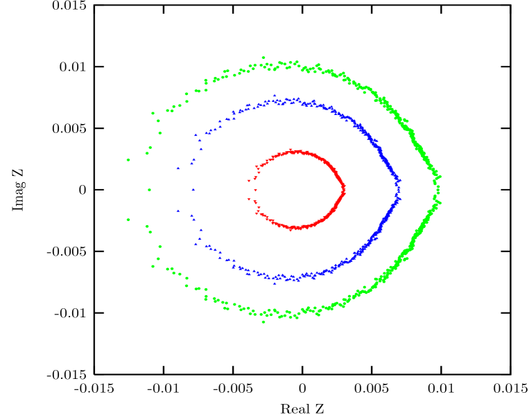
Figure 2: The difference spectra of the overlap operator with $\delta=0$ and the operators with $\delta=0.01$ (most outer spectrum), $\delta=0.001$ (middle spectrum) and $\delta=0.0001$ (most inner spectrum). The difference spectra for $\delta=0.001$ and $\delta=0.0001$ have been scaled with a factor $7$ and $30$, respectively, in order to be able to include them in the plot.

The smallness of the distortions in the spectrum as observed in fig. 2 appears to be quite promising for this choice of an approximate overlap operator. However, the effects on the fluctuations are considerable as can be seen in fig. 3. For a value of $\delta=0.0001$ (circles) the determinant ratio ${R_{\mathrm{det}}}\approx 1$ and has very small fluctuations until the degree of the polynomial is lowered to ${\tilde{n}}=8$ which is a factor of three smaller than the original degree of the polynomial. However, already for $\delta=0.001$ (upward triangles) ${R_{\mathrm{det}}}$ starts to develop some fluctuations and finally, for $\delta=0.01$ (downward triangles) the fluctuations are becoming so large that realistic simulations with such a value of $\delta$ cannot be performed.

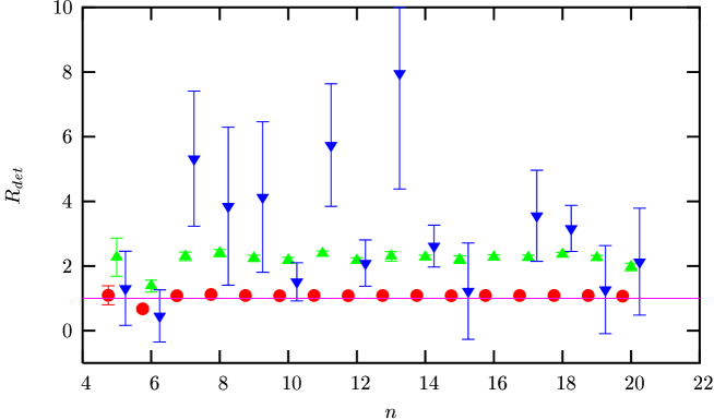
Figure 3: The determinant ratio ${R_{\mathrm{det}}}$ as a function of the degree $n$ of the Chebyshev polynomial. We plot the cases for $\delta=0.0001$ (circles), $\delta=0.001$ (upward triangles) and $\delta=0.01$ (downward triangles).

As a conclusion, we found that none of the above described attempts led to a satisfactory solution for an infrared safe dynamical overlap simulation. As said above, we therefore have performed the overlap simulations finally by generating pure gauge configuration and using a reweighting with the determinant, computed exactly from the eigenvalues.

Summary of simulation setup

In the following table we shortly summarize which technique we have used for the different lattice fermions for the simulations and for the observables.

	Wilson / tm / hypercube	overlap
simulations	standard HMC	determinant reweighting
operators	conjugate gradient solver	eigenvalues
		& eigenvectors/
		conjugate gradient solver
currents	local / conserved	local
pseudo scalar correlator	$\langle\mathcal{PP}\rangle$	$\langle\mathcal{PP}-\mathcal{SS}\rangle$
scalar condensate	Ward-Takahashi-identity	$\langle\bar{\psi}(1-\frac{a}{2}D)\psi\rangle$

Let us end this section by a small technical remark. For the computations of the eigenvalues and eigenvectors we used the LAPACK [36] routine. In the course of our work we found that this routine does not compute correctly the eigenvectors in the case of degenerate zero modes. It rather gives linear combinations of the exact solutions which led to a problem in the computation of the pseudo scalar correlator using the operator $\mathcal{P}$ if configurations with topological charge $|Q|>1$ are considered. The effect shows up in such a way that the pseudo scalar correlator eq. (16) develops a plateau like behaviour for values of Euclidean time $t$ close to the middle of the lattice. This behaviour made it practically impossible to extract the pseudo scalar mass and the PCAC fermion mass. By re-diagonalizing the zero mode sector we could verify that this effect goes away.

As a simple solution for our simulations we decided to always take the correlator $\langle\mathcal{P}(t)\mathcal{P}(0)-\mathcal{S}(t)\mathcal{S}(0)\rangle$ in which this zero mode contribution is cancelled out [37]. The only exception is the case $z=0.8$, where the pseudo scalar masses are so high that it became very difficult to disentangle them from the scalar masses when the $\langle\mathcal{S}(t)\mathcal{S}(0)\rangle$ was subtracted of. Therefore we used for this large value of $z$ the conjugate gradient solver to compute the correlators.

4 Results

It is the main aim of this paper to check the scaling behaviour of the fermion actions described in section 2. To this end, we have chosen the simulation parameters such that we fix the scaling variable

$$z\equiv\left(m_{f}/g\right)^{2/3}=\left(m_{f}\sqrt{\beta}\right)^{2/3}\;.$$ (40)

We performed simulations for a wide range of $\beta$-values, $0.1\leq\beta\leq 6$. For Wilson, hypercube and twisted mass fermions our lattices were mainly of size $V=L^{2}=32^{2}$. Only at $\beta=5,6$ and $z=0.2$ we went up to $V=48^{2}$ lattices. For the overlap fermion simulations we mainly used $V=20^{2}$ and, for $z=0.2$, $V=24^{2}$ lattices. Only at $\beta=5$ and $z=0.2$ we used a $V=28^{2}$ lattice. It is our experience that for larger lattices the determinant reweighting technique used for the overlap fermion simulations are not practical since they lead to large fluctuations which spoil the signal to noise ratio. We finally mention that all our error analyzes are based on the method described in ref. [38] including thus the autocorrelation times in the computation of the errors.

As a prime quantity we will test the scaling behaviour of $m_{\pi}\sqrt{\beta}$, performing finally a continuum limit for all actions used. In the continuum, there are two approximate calculations for $m_{\pi}^{\mathrm{cont}}/e$ for the massive Schwinger model.

The first is performed by Smilga [39] who finds for strong coupling and small fermion mass

$$\frac{m_{\pi}^{\mathrm{cont}}}{e} \approx 2^{5/6}\text{e}^{\gamma/3}\Big{(}\frac{\Gamma(3/4)}{\Gamma(1/4)}\Big{)}^{2/3}\frac{\Gamma(1/6)}{\Gamma(2/3)}\Big{(}\frac{m}{e}\Big{)}^{2/3}$$ (41)

$$= 2.008\Big{(}\frac{m}{e}\Big{)}^{2/3}\;.$$ (42)

For large masses, Gattringer in ref. [40] finds from a semi-classical analysis

$$\frac{m_{\pi}^{\mathrm{cont}}}{e} \approx \text{e}^{2\gamma/3}\frac{2^{5/6}}{\pi^{1/6}}\Big{(}\frac{m}{e}\Big{)}^{2/3}$$ (43)

$$= 2.163\Big{(}\frac{m}{e}\Big{)}^{2/3}\;.$$ (44)

Note that we give these results in terms of the dimensionful quantities, coupling $e$, fermion mass $m$ and pseudo scalar mass $m_{\pi}^{\mathrm{cont}}$. Both expression are approximate computations and it is interesting to compare these against our non-perturbative calculations.

For completeness, we also give here analytical expressions for the scalar condensate as available in the literature. The first is again from ref. [39],

$$\frac{\Sigma^{\mathrm{cont}}}{e}\approx 0.388\Big{(}\frac{m}{e}\Big{)}^{1/3}\;.$$ (45)

A second expression is derived in ref. [41],

$$\frac{\Sigma^{\mathrm{cont}}}{e}=\frac{1}{4\pi}\frac{(m_{\pi}^{\mathrm{cont}}/e)^{2}}{(m/e)}\;.$$ (46)

Critical fermion mass

For Wilson fermions and for hypercube fermions, the fermion mass receives an additive renormalization. Therefore, the critical values of the bare fermion mass, where e.g. the PCAC fermion mass vanishes has to be determined by non-perturbative simulations. We computed $m_{\mathrm{PCAC}}$, extracted from eq. (31) using the conserved currents of eqs. (32,33) as a function of the bare fermion masses, $m_{0}$ for Wilson and $m_{\mathrm{hyp}}$ for hypercube fermions. We determined at each value of $\beta$ those values of $m_{0}$ and $m_{\mathrm{hyp}}$ where $m_{\mathrm{PCAC}}=0$. The value of these bare fermion masses can be found in table 4. Note that the actual critical mass values used for the twisted mass simulations in order to realize full twist, though compatible, differ slightly from the ones in table 4 since they were obtained with less statistics.

$\beta$	$-m_{\mathrm{crit}}^{\mathrm{Wilson}}$	$-m_{\mathrm{crit}}^{\mathrm{hyp}}$
1.0	0.3204(7)	0.335(1)
2.0	0.1968(9)	0.203(1)
3.0	0.1351(2)	0.1392(4)
4.0	0.1033(1)	0.1050(2)
5.0	0.0840(1)	0.0856(1)
6.0	0.0719(1)	0.0727(1)

Table 1: Critical hopping parameters at the values of $\beta$ used in our simulations for the Wilson, $m_{\mathrm{crit}}^{\mathrm{Wilson}}$, and hypercube, $m_{\mathrm{crit}}^{\mathrm{hyp}}$, fermions.

Fermion mass dependence of the pion mass

As described above, in the scaling analysis we will fix the scaling variable $z=\left(m_{f}\sqrt{\beta}\right)^{2/3}$. To this end, we first explored the dependence of the pion mass as a function of the PCAC fermion mass for fixed values of $\beta$. We give one example for the case of hypercube fermions in fig. 4 using the conserved currents of eqs. (32,33) to compute the PCAC fermion mass. We also plot in the graph the analytic predictions of eqs. (41,43) for the fermion mass dependence of the pion mass.

The data in fig. 4 are for $\beta=0.1$, $\beta=0.5$ and $\beta=1.0$. Clearly, for $\beta=0.1$ the data do not follow the theoretical expectation while for the other values of $\beta$ there seems to be some agreement with the analytical formulae. However, in order to make more definite statements, a closer look to the scaling behaviour is clearly needed. Anyhow, the main purpose of fig. 4 is to show that we have collected data that are concentrated around the values of $z=0.2$, $z=0.4$ and $z=0.8$ that we are interested in for our final scaling analysis. When the values of $z$ did not coincide directly with the desired ones, we performed an only very small linear interpolation of our data to achieve the exact values of $z$.

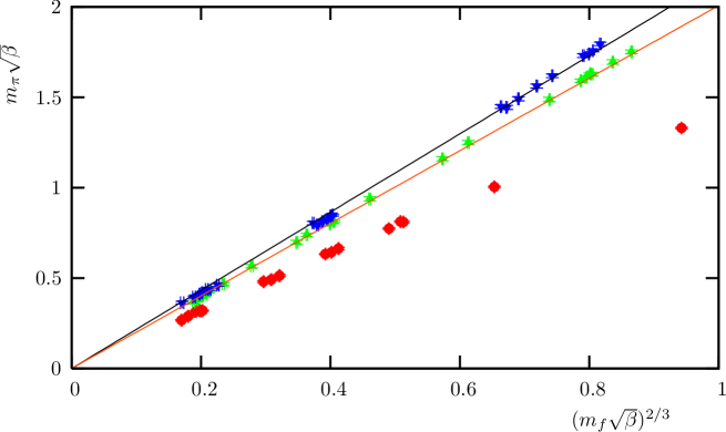
Figure 4: Pseudo scalar mass $m_{\pi}\sqrt{\beta}$ versus $z=(m_{f}\sqrt{\beta})^{2/3}$ for three values of $\beta$. The solid lines are the analytical predictions of eqs. (41,43). Crosses represent our data for $\beta=1$, triangles for $\beta=0.5$ and diamonds for $\beta=0.1$.

Finite size effects

One source of a systematic error in the determination of $m_{\pi}$ are possible finite size effects. For two dimensions the asymptotic finite size corrections for the pseudo scalar mass were computed in ref. [42] and studied numerically in the case of the Schwinger model in ref. [4]. A very good agreement to the theoretical prediction was found and it was observed that the variable $m_{\pi}L$ needs to be surprisingly large to suppress finite size corrections.

Taking this as a warning, we followed the procedure of ref. [4] and performed a finite size correction of our values for the pseudo scalar masses when necessary. We used the analytical formula

$$m_{\pi}(L)=m_{\pi}^{\infty}+A\frac{\sqrt{m_{\pi}^{\infty}}}{\sqrt{L}}e^{-Lm_{\pi}^{\infty}}$$ (47)

where $m_{\pi}^{\infty}$ denotes the pseudo scalar mass in the infinite volume limit. Rescaling eq. (47) by $\sqrt{\beta}$ this formula can be applied to all our finite volume data at various, large enough values of $\beta$ to keep the effects of the lattice spacing small. Inspecting our data, we decided to perform a global fit to our simulation data obtained with Wilson, hypercube and Wilson twisted mass fermions at $z=0.2$ and $z=0.4$ for $\beta\geq 4$. As a result we found a “universal” constant $A=12.4(6)$ which is compatible with the value computed in ref. [4]. In fig. 5 we give an example for the resulting fit for a subset of our data in the case of Wilson fermions.

We then examined all pseudo scalar masses that we will use in the detailed scaling analysis described below and used eq. (47) to analytically correct for finite size effects. We give in tables 2, 3 and 4 the infinite volume values for the pseudo scalar mass as obtained from this finite size correction. Note that in most of the cases, this correction is negligibly small and stays anyhow on the percent level.

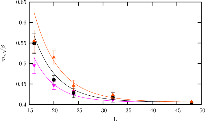
Figure 5: We show $m_{\pi}\sqrt{\beta}$ as a function of $L$ at the example of Wilson fermions and three values of $\beta$ (downward triangles: $\beta=4$, circles: $\beta=5$, upward triangles: $\beta=6$). The fit curves, represented by solid lines, are obtained by performing a common fit to eq. (47) to our data for $z=0.2$ and $z=0.4$ and for Wilson, hypercube and twisted mass fermions, choosing always $\beta\geq 4$.

Wilson fermion results
$z$	$\beta$	$m_{0}^{\mathrm{local}}$	$m_{0}^{\mathrm{cons}}$	$L$	$m_{\pi,\infty}^{\mathrm{local}}\sqrt{\beta}$	$m_{\pi,\infty}^{\mathrm{cons}}\sqrt{\beta}$	$\Sigma_{\mathrm{sub}}^{\mathrm{cons}}\sqrt{\beta}$
0.2	1.0	-0.231367	-0.230193	32	0.388(5)	0.391(3)	0.277(7)
0.2	2.0	-0.132316	-0.131842	32	0.402(3)	0.406(2)	0.252(6)
0.2	3.0	-0.082626	-0.081935	32	0.404(4)	0.408(2)	0.232(7)
0.2	4.0	-0.057374	-0.056979	32	0.406(2)	0.408(2)	0.231(8)
0.2	5.0	-0.043199	-0.043010	48	0.403(2)	0.404(1)	0.219(6)
0.2	6.0	-0.034249	-0.034009	48	0.404(2)	0.406(2)	0.225(4)
0.4	1.0	-0.075308	-0.059286	32	0.75(1)	0.779(5)	0.339(6)
0.4	2.0	-0.017495	-0.008352	32	0.783(8)	0.813(6)	0.339(3)
0.4	3.0	0.014505	0.019789	32	0.799(7)	0.819(3)	0.334(4)
0.4	4.0	0.026358	0.031078	32	0.80(1)	0.820(3)	0.340(3)
0.4	5.0	0.032526	0.035391	32	0.808(4)	0.824(2)	0.345(2)
0.4	6.0	0.036146	0.037693	32	0.811(3)	0.820(2)	0.345(2)
0.8	1.0	0.352443	0.537801	32	1.36(1)	1.560(5)	0.329(1)
0.8	2.0	0.314017	0.403487	32	1.52(1)	1.690(5)	0.400(1)
0.8	3.0	0.298677	0.350958	32	1.60(1)	1.729(4)	0.438(1)
0.8	4.0	0.276568	0.314133	32	1.63(1)	1.745(5)	0.469(1)
0.8	5.0	0.255009	0.285628	32	1.65(1)	1.758(3)	0.494(1)
0.8	6.0	0.239625	0.262974	32	1.686(6)	1.770(3)	0.518(1)

Table 2: Results for the Wilson fermion simulations. The scaling variable $\left(m_{f}\sqrt{\beta}\right)^{2/3}$ is fixed by using either the local or the conserved currents to determine the PCAC fermion mass resulting in the two different values of the pseudo scalar mass. Typical statistics of the runs were between $4000$ and $10000$ configurations.

Hypercube fermion results
$z$	$\beta$	$m_{0}^{\mathrm{local}}$	$m_{0}^{\mathrm{cons}}$	$L$	$m_{\pi,\infty}^{\mathrm{local}}\sqrt{\beta}$	$m_{\pi,\infty}^{\mathrm{cons}}\sqrt{\beta}$	$\Sigma_{\mathrm{sub}}^{\mathrm{cons}}\sqrt{\beta}$
0.2	1.0	-0.237698	-0.231044	32	0.39(1)	0.416(3)	0.290(6)
0.2	2.0	-0.137038	-0.133369	32	0.400(3)	0.416(3)	0.264(7)
0.2	3.0	-0.085462	-0.083199	32	0.400(7)	0.415(2)	0.250(6)
0.2	4.0	-0.059364	-0.058095	32	0.399(9)	0.416(2)	0.240(5)
0.2	5.0	-0.044387	-0.043885	48	0.408(2)	0.410(2)	0.246(8)
0.2	6.0	-0.035528	-0.034893	32	0.413(7)	0.411(7)	0.247(4)
0.4	1.0	-0.083223	-0.045098	32	0.78(2)	0.844(9)	0.375(2)
0.4	2.0	-0.025253	-0.004337	32	0.78(1)	0.846(4)	0.381(2)
0.4	3.0	0.012877	0.021147	32	0.806(6)	0.836(3)	0.382(2)
0.4	4.0	0.025787	0.031202	32	0.809(4)	0.834(4)	0.385(2)
0.4	5.0	0.031525	0.035539	32	0.812(3)	0.831(2)	0.392(3)
0.4	6.0	0.034082	0.037392	32	0.816(3)	0.835(2)	0.392(3)
0.8	1.0	0.311570	0.613589	32	1.39(2)	1.742(6)	0.366(1)
0.8	2.0	0.309020	0.433230	32	1.55(2)	1.792(6)	0.466(1)
0.8	3.0	0.293918	0.365237	32	1.61(1)	1.793(4)	0.517(1)
0.8	4.0	0.272609	0.321868	32	1.65(1)	1.792(5)	0.557(1)
0.8	5.0	0.255540	0.290832	32	1.672(7)	1.792(4)	0.588(1)
0.8	6.0	0.237752	0.266771	32	1.68(1)	1.796(5)	0.616(1)

Table 3: Results for the hypercube fermion simulations. The scaling variable $\left(m_{f}\sqrt{\beta}\right)^{2/3}$ is fixed by using either the local or the conserved currents to determine the PCAC fermion mass resulting in the two different values of the pseudo scalar mass. Typical statistics of the runs were between $4000$ and $10000$ configurations.

Twisted mass fermion results
$z$	$\beta$	$m_{0}^{\mathrm{local}}$	$m_{0}^{\mathrm{cons}}$	$L$	$m_{\pi,\infty}^{\mathrm{local}}\sqrt{\beta}$	$m_{\pi,\infty}^{\mathrm{cons}}\sqrt{\beta}$	$\Sigma_{\mathrm{sub}}^{\mathrm{cons}}\sqrt{\beta}$
0.2	1.0	-	0.071591	32	-	0.434(2)	0.303(7)
0.2	2.0	0.050499	0.054990	32	0.408(8)	0.428(2)	0.271(10)
0.2	3.0	0.045007	0.046886	32	0.411(2)	0.422(2)	0.249(6)
0.2	4.0	-	0.041533	32	-	0.421(1)	0.226(6)
0.2	5.0	0.036965	0.037643	48	0.409(2)	0.414(2)	0.237(5)
0.2	6.0	-	0.034651	48	-	0.414(2)	0.233(7)
0.4	1.0	0.177303	0.208213	32	0.78(1)	0.874(3)	0.446(7)
0.4	2.0	0.144653	0.157190	32	0.81(1)	0.867(3)	0.412(4)
0.4	3.0	0.125186	0.133453	32	0.819(8)	0.851(2)	0.394(4)
0.4	4.0	0.113557	0.117956	32	0.824(4)	0.846(2)	0.385(5)
0.4	5.0	0.102819	0.106827	32	0.820(4)	0.844(2)	0.388(4)
0.4	6.0	0.095373	0.098326	32	0.821(3)	0.842(2)	0.393(5)
0.8	1.0	0.471381	0.654028	32	1.47(2)	1.799(5)	0.571(2)
0.8	2.0	0.376485	0.459309	32	1.60(1)	1.856(3)	0.628(2)
0.8	3.0	0.334417	0.384597	32	1.66(2)	1.838(3)	0.638(2)
0.8	4.0	0.306509	0.337947	32	1.695(6)	1.835(3)	0.659(2)
0.8	5.0	0.282663	0.305270	32	1.719(6)	1.829(3)	0.671(2)
0.8	6.0	0.262653	0.280421	32	1.731(6)	1.833(3)	0.683(2)

Table 4: Results for the Wilson maximally twisted mass fermion simulations. The scaling variable $\left(m_{f}\sqrt{\beta}\right)^{2/3}$ is fixed by using either the local or the conserved currents to determine the PCAC fermion mass resulting in the two different values of the pseudo scalar mass. Typical statistics of the runs were between $4000$ and $10000$ configurations.

Overlap fermion results
$\beta$	$m_{\mathrm{ov}}$	$(m_{\mathrm{ov}}\sqrt{\beta})^{2/3}$	$(m_{f}^{\mathrm{local}}\sqrt{\beta})^{2/3}$	$L$	$m_{\pi,\infty}^{\mathrm{local}}\sqrt{\beta}$	$\Sigma\sqrt{\beta}$
3.0	0.0464758	0.1864	0.194(15)	24	0.37(4)	0.176(4)
4.0	0.0447214	0.2000	0.200(8)	24	0.42(4)	0.177(4)
5.0	0.0420000	0.2066	0.20(3)	28	0.46(4)	0.138(2)
1.0	0.2529822	0.4000	0.4061(14)	20	0.807(16)	0.1950(16)
2.0	0.1788854	0.4000	0.4069(19)	20	0.824(14)	0.2340(12)
3.0	0.1460595	0.4000	0.399(2)	20	0.851(12)	0.2518(7)
4.0	0.1264911	0.4000	0.383(2)	20	0.833(10)	0.2618(7)
5.0	0.1142685	0.4027	0.396(5)	24	0.837(10)	0.2415(8)
1.0	0.5724334	0.6894	0.797(2)	20	1.433(10)	0.2363(3)
2.0	0.4232769	0.7103	0.8047(5)	20	1.568(4)	0.2905(3)
3.0	0.3553500	0.7236	0.7934(2)	20	1.604(3)	0.3270(3)
4.0	0.3152474	0.7353	0.7916(1)	20	1.638(2)	0.3549(3)
5.0	0.2916839	0.7521	0.8010(2)	20	1.682(2)	0.3811(6)

Table 5: Results for the overlap fermion simulations. The scaling variable $\left(m_{f}\sqrt{\beta}\right)^{2/3}$ is fixed by using the local currents to determine the PCAC fermion mass. We give for comparison also the values of the scaling variable $z$ when the bare overlap fermion mass $m_{\mathrm{ov}}$ is used. Typical statistics of the runs were $4000$ configurations.

4.1 Results for the pseudo scalar mass

In tables 2, 3 and 4 we give our results for the pseudo scalar masses at fixed scaling variable $z$ of eq. (40), where $z$ is fixed either by using local or conserved currents to extract the PCAC fermion mass. While in the tables we give only the results for $\beta\geq 1$, we have performed simulations also for smaller values of $\beta$ for all actions, except overlap fermions. We show the result for $m_{\pi}\sqrt{\beta}$ as a function of $\beta$ in fig. 6. The graph is done for the example of $z=0.4$ where we used the conserved currents to determine the PCAC fermion mass. Clearly, large lattice cut-off effects are observed when small values of $\beta<1$ are taken. From the figure it is obvious that for an asymptotic scaling analysis values of $\beta\geq 1$ should be taken.

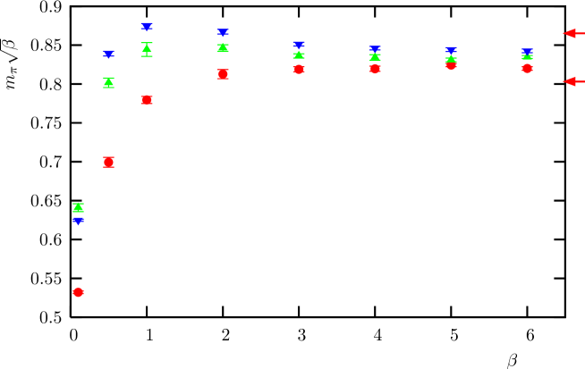
Figure 6: We show $m_{\pi}\sqrt{\beta}$ as a function of $\beta$ at fixed value of $z=0.4$ as determined from the PCAC fermion mass employing conserved currents. We represent results from Wilson fermions by circles, from twisted mass fermions by downward and for hypercube fermions by upward triangles. The arrows represent the theoretical prediction, the upper arrow is from eq. (43) the lower from eq. (41).

In figs. 7, 8 and 9 we show the results of our scaling test for fixed $z=0.8$, $z=0.4$ and $z=0.2$ respectively. For the values of $\beta=1$ and $\beta=2$ at $z=0.2$, the determinant used for reweighting the overlap results induced large fluctuations such that no reliable values of physical observables could be extracted. For all figures the value of $z$ was determined using local currents to compute the PCAC fermion mass. We show $m_{\pi}\sqrt{\beta}$ as a function of $1/\beta\propto a^{2}$. We first performed linear fits in $1/\beta$ independently for each lattice fermion used. Since these fits gave consistent continuum values for $m_{\pi}\sqrt{\beta}$ for all actions, see the example for $z=0.4$ in ref. [35], we finally performed constraint fits, demanding that all actions give the same continuum value for $m_{\pi}\sqrt{\beta}$ at fixed value of $z$. We show these constraint fits in figs. 7, 8 and 9 as the solid lines. The data for all kind of fermions, Wilson, hypercube, maximally twisted mass and overlap, are nicely consistent with a linear behaviour in $a^{2}$. While this is expected for maximally twisted mass and overlap fermions, this outcome is somewhat surprising for hypercube and Wilson fermions. Note that our finding for Wilson fermions is, however, consistent with the results in ref. [43].

Figure 7: Scaling test of $m_{\pi}\sqrt{\beta}$ as function of $1/\beta\propto a^{2}$ at fixed value of $z=0.8$. The solid lines represent linear constraint fits in $1/\beta$ demanding the same continuum limit value for all kind of lattice fermions used. For Wilson, hypercube and twisted mass fermions we used data obtained at $\beta\geq 3$, while for overlap fermions data with $\beta\geq 2$ were used.

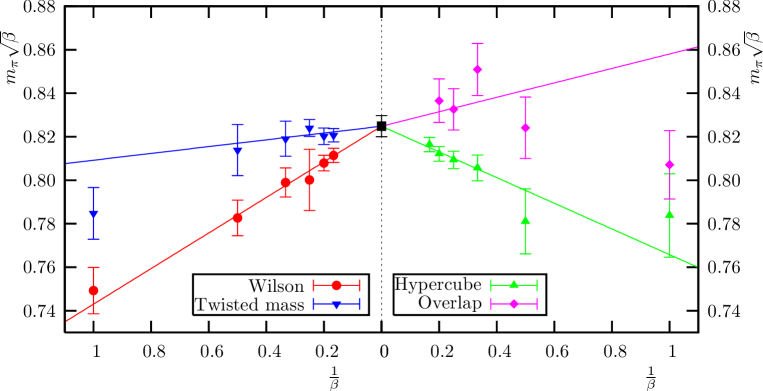
Figure 8: Scaling test of $m_{\pi}\sqrt{\beta}$ as function of $1/\beta\propto a^{2}$ at fixed value of $z=0.4$. The solid lines are fits explained in fig. 7.

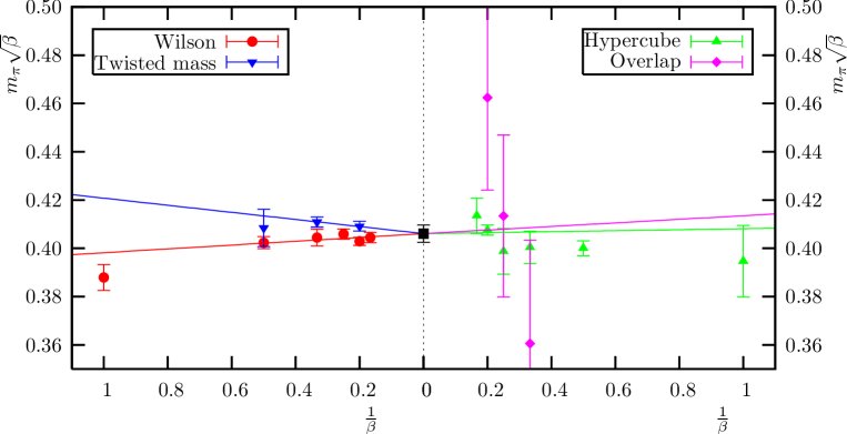
Figure 9: Scaling test of $m_{\pi}\sqrt{\beta}$ as function of $1/\beta\propto a^{2}$ at fixed value of $z=0.2$. The solid lines are fits explained in fig. 7.

In general it is very difficult to decide which kind of lattice fermion shows the best scaling behaviour and we cannot draw a definite conclusion here. First of all, all kind of fermions show only small lattice artefacts. Second, if one would use the PCAC fermion mass from the conserved currents, the picture changes. We give an example for $z=0.4$ in fig. 10 which reveals again an O(a²) scaling for the here used Wilson, maximally twisted mass and hypercube fermions. When compared to fig. 8 where maximally twisted mass fermions show the smallest scaling violations, in fig. 10 hypercube fermions seem to do better.

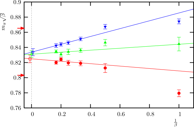
Figure 10: Scaling of $m_{\pi}\sqrt{\beta}$ as function of $1/\beta$ using conserved currents to compute the PCAC fermion mass to fix $z=0.4$. We denote by circles Wilson, by downward triangles twisted mass and by upward triangles hypercube fermions. The solid lines represent linear fits in $1/\beta$ for $\beta\geq 3$. The arrows represent the theoretical prediction, the upper arrow is from eq. (43) the lower from eq. (41).

Continuum comparison to theory

As was shown above, all kind of fermions show a nice scaling behaviour that is linear in $a^{2}$ and give a universal continuum limit. In fig. 11 we show $m_{\pi}\sqrt{\beta}$ as a function of $z$ in the continuum and compare to the theoretical expectations of eq. (41) (lower line) and eq. (43) (upper line). As an inlay we plot the ratio $R_{m_{\pi}}=m_{\pi}^{\mathrm{data}}/m_{\pi}^{\mathrm{theor}}$ of our non-perturbatively obtained data extrapolated to the continuum and the two theoretical predictions. Triangles represent the data divided by the corresponding value computed from eq. (43) while circles represent the data divided by the corresponding value computed from eq. (41). To the precision we could obtain in this work, the theoretical predictions do not describe the non-perturbatively obtained simulation data satisfactory at all values of $z$. Only for small values of the fermion mass ($z=0.2$) there seems to be some agreement with eq. (41) while at $z=0.8$ eq. (43) seems to hold only.

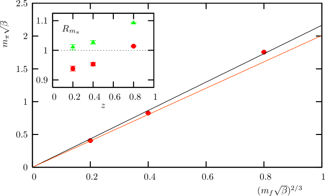
Figure 11: Continuum behaviour of $m_{\pi}\sqrt{\beta}$ as function of z. The lower curve represents eq. (41), the upper curve eq. (43). The inlay gives the ratio $R_{m_{\pi}}$ of our non-perturbatively obtained data and the two theoretical calculations. Triangles use eq. (43) and circles use eq. (41).

4.2 Scalar Condensate

Another physical quantity we will consider in this work is the scalar condensate $\Sigma\equiv\langle\bar{\psi}\psi\rangle$, for which analytical predictions exist, see eq. (45) and eq. (46). A very simple way to calculate the scalar condensate is to compute

$$\Sigma=\frac{1}{V}\sum_{x}\mathrm{Tr}D^{-1}(x,x)$$ (48)

using a stochastic method. We denote the so computed values of $\Sigma$ as $\Sigma_{\mathrm{direct}}$. A severe drawback of this definition of $\Sigma$ is that, at least in the case of Wilson and hypercube fermions, from the mixing with the identity operator a divergent piece $\propto 1/a$ appears that needs to be subtracted non-perturbatively.

In the case of the twisted mass fermions at full twist, it is possible to use the operator $\langle\bar{\psi}\sigma_{3}\tau_{3}\psi\rangle$, i.e. the 3rd component of the pseudo scalar operator (see eq. (16)), for the calculation of the scalar condensate. This operator does not mix with the identity operator and thus the divergent piece does not appear.

Also for the overlap operator there is a definition $\Sigma_{\mathrm{ov}}\equiv\langle\bar{\psi}(1-\frac{a}{2}D_{\rm ov}^{(0)}\psi\rangle$ which subtracts of the divergent piece automatically. For overlap fermions, we calculated therefore directly the scalar condensate from the eigenvalues of $D_{\mathrm{ov}}$

$$\Sigma_{\mathrm{ov}}=\frac{1}{V}\langle\sum_{i}\frac{1}{\lambda_{i}}(1-\lambda_{i}(0)/2)\rangle\;,$$ (49)

where $\lambda_{i}$ denotes an eigenvalue of the massive overlap operator and $\lambda_{i}(0)$ denotes an eigenvalue at zero fermion mass, i.e. the eigenvalues of $D_{\rm ov}^{(0)}$.

A second way, which avoids the appearance of the divergent piece from the beginning, is to compute a so-called subtracted scalar condensate $\Sigma_{\mathrm{sub}}$ using the integrated axial Ward-Takahashi identity [30],

$$\Sigma_{\mathrm{sub}}=2m_{\mathrm{PCAC}}\sum_{x}\langle\mathcal{\tilde{P}}_{x}\mathcal{\tilde{P}}_{0}\rangle\;.$$ (50)

In the twisted mass case, this corresponds to the integrated PCVC relation

$$\Sigma_{\mathrm{sub}}=\langle\bar{\psi}\sigma_{3}\tau_{3}\psi\rangle_{\mathrm{sub}}=2m_{\mathrm{PCVC}}\sum_{x}\langle\mathcal{\tilde{P}}_{x}\mathcal{\tilde{P}}_{0}\rangle\;.$$ (51)

Comparison of $\Sigma_{\mathrm{direct}}$ and $\Sigma_{\mathrm{sub}}$

To just illustrate the effect of using a direct and a subtracted definition of the scalar condensate, we plot $\Sigma_{\mathrm{direct}}$ and $\Sigma_{\mathrm{sub}}$ for Wilson and maximally twisted mass fermions in fig. 12.

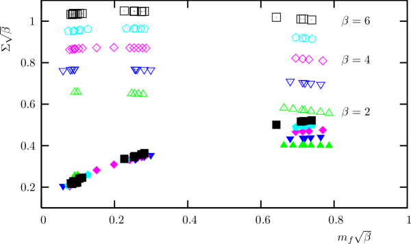
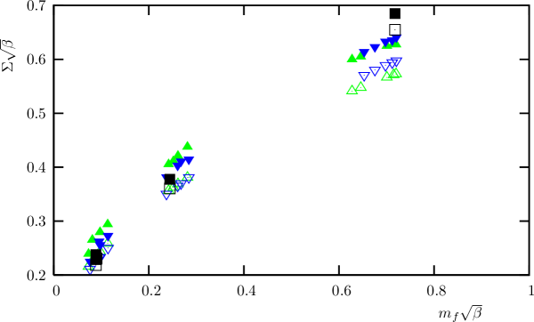
Figure 12: The condensate from the direct $\Sigma_{\mathrm{direct}}$ (open symbols) and the subtracted $\Sigma_{\mathrm{sub}}$ (full symbols) determinations. Error bars are within the size of the symbols. Upper graph: $\Sigma_{\mathrm{direct}}$ and $\Sigma_{\mathrm{sub}}$ for Wilson fermion. We indicate the values of $\beta$ where $\Sigma_{\mathrm{direct}}$ is obtained. Lower graph: $\Sigma_{\mathrm{direct}}$ and $\Sigma_{\mathrm{sub}}$ for twisted mass fermions. In this case, the results from both condensates are consistent up to scaling violations.

In two dimensions, there is in general a relation between $\Sigma_{\mathrm{direct}}$ and $\Sigma_{\mathrm{sub}}$ given by

$$\Sigma_{\mathrm{sub}}=\Sigma_{\mathrm{direct}}-c_{0}/a\,.$$ (52)

The coefficient $c_{0}$ multiplying the $1/a$ divergence is to be determined non-perturbatively. In the upper panel of fig. 12, the $1/a$ dependence is clearly visible for $\Sigma_{\mathrm{direct}}$, as for increasing values of $\beta$, the values of $\Sigma_{\mathrm{direct}}$ increase accordingly. It is clear from the figure that an extraction of a physical value for the scalar condensate will be very difficult since the term $c_{0}/a$ dominates the signal.

According to [30], $c_{0}$ comes from the explicit breaking term of chiral symmetry for Wilson fermions. Therefore, one can expect that for twisted mass fermions at maximal twist this term is absent and $\Sigma_{\mathrm{direct}}$ behaves like $\Sigma_{\mathrm{sub}}$. This is shown in the lower panel of fig. 12. In the case of twisted mass fermions both $\Sigma_{\mathrm{direct}}$ and $\Sigma_{\mathrm{sub}}$ are comparable (modulo scaling violations). In fact, we find a tendency that the ratio $\Sigma_{\mathrm{sub}}/\Sigma_{\mathrm{direct}}$ approaches one when $\beta$ is increased. We finally remark that also for the improved definition of the scalar condensate of eq. (49) in case of overlap fermions the divergence term is automatically subtracted of. As a result of this discussion we will calculate the scalar condensate from the subtracted scalar condensate in the case of Wilson, hypercube and maximally twisted mass fermions while for overlap fermions we will use the direct calculation with the improved definition.

Scaling of the scalar condensate

Let us now turn to the results of the scaling behaviour of the scalar condensate for the various fermion actions. We show the results in fig. 13. $\Sigma_{\mathrm{sub}}$ is calculated for Wilson, hypercube and twisted mass fermion, and $\Sigma_{\mathrm{direct}}$ is done for overlap fermions, at $z=(m_{f}\sqrt{\beta})^{2/3}=0.2$, 0.4 and 0.8.

     

     

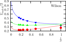
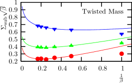
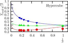
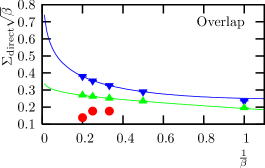
Figure 13: Scaling of the scalar condensate as a function of $1/\beta$ at $z=0.2$ (circles), $z=0.4$ (upper triangles) and $z=0.8$ (downward triangle). The solid lines represent the fits using eq. (54) for $\beta\geq 2$.

The figures show a strong dependence of the scalar condensate on $1/\beta$, in particular for the heavy fermion region. This behaviour can be explained by the fact that in two dimensions, the scalar condensate develops a logarithmic divergence in $\beta$ when the lattice spacing is sent to zero . This is most easily seen in the free theory where a simple computation of the scalar condensate leads to a behaviour (see also ref. [5])

$$\frac{\Sigma_{\mathrm{free}}}{e}\propto\frac{m}{e}\log\left(\frac{1/a^{2}+m^{2}}{m^{2}}\right)=\frac{m}{e}\log\left(\frac{\beta+(m/e)^{2}}{(m/e)^{2}}\right)\;,$$ (53)

where we have inserted $\beta=1/a^{2}e^{2}$ and $m$ denotes the continuum fermion mass. Fixing $m/e$, as we do in this work, and approaching the continuum limit by letting $\beta\rightarrow\infty$, a logarithmic increase of the scalar condensate in $\beta$ will appear. Fig. 13 shows clearly such an behaviour for all actions we have employed.

It is therefore natural to use a fit ansatz of the form

$$\Sigma=A+\frac{B}{\beta}+C\log{\frac{1}{\beta}}.$$ (54)

In fig. 13 we show also the fit to the data using eq. (54). For $z=0.2$ we could not extract reliable values for $\Sigma$ at $\beta=1,2$ since the determinant induced very large fluctuations. Since we were then left with only three data points for a three parameter fit, and we were also not sure whether the values for $\Sigma$ are possibly affected by finite size effects, we did not use the fit in eq.(47) for overlap fermions at $z=0.2$.

As can be seen, this fit function provides a nice description of the numerical data. In principle, for the cases of twisted mass and overlap fermions the divergent piece can be subtracted of from the evaluation of this term in the free theory when the fermion mass is matched. This is, however, very difficult for the cases of Wilson and hypercube fermions since there the matching of the fermion mass is not unique. We give in table 6 the fit results using eq. (54).

$\Sigma=A+\frac{B}{\beta}+C\log(\frac{1}{\beta})$
$(m\sqrt{\beta})^{2/3}=0.2$	$A$	$B$	$C$	$\chi^{2}$/dof
Wilson	0.118(103)	0.215(150)	-0.0397(447)	0.56
HYP	0.0938(898)	0.259(134)	-0.0610(389)	0.52
TM	0.0352(1189)	0.371(179)	-0.0767(518)	1.7
$(m\sqrt{\beta})^{2/3}=0.4$	$A$	$B$	$C$	$\chi^{2}$/dof
Wilson	0.258(52)	0.107(76)	-0.0396(229)	0.67
HYP	0.316(38)	0.0790(543)	-0.0357(174)	0.48
TM	0.218(69)	0.293(98)	-0.0698(307)	0.47
OV	0.249(19)	-0.0565(271)	-0.0200(83)	0.13
$(m\sqrt{\beta})^{2/3}=0.8$	$A$	$B$	$C$	$\chi^{2}$/dof
Wilson	0.235(14)	0.129(21)	-0.145(6)	0.62
HYP	0.311(14)	0.0843(207)	-0.162(6)	0.19
TM	0.465(31)	0.178(45)	-0.106(14)	2.4
OV	0.128(10)	0.136(18)	-0.160(4)	0.022

Table 6: Fit results for the scalar condensate using eq. (54)

5 Conclusions

In this paper we have tested four different lattice fermions in their approach to the continuum limit in the 2-dimensional massive Schwinger model with $N_{f}=2$ flavours of dynamical fermions. At fixed scaling variable $z=(m_{f}\sqrt{\beta})^{2/3}=0.2,0.4,0.8$ we have computed the pseudo scalar mass $m_{\pi}\sqrt{\beta}$ and the scalar condensate $\Sigma$ for various values of $\beta=1/e^{2}a^{2}$.

For all kind of fermions used, Wilson, hypercube, twisted mass and overlap fermions, the scaling behaviour of $m_{\pi}\sqrt{\beta}$ appears to be linear in $a^{2}$. While this is expected for twisted mass fermions at full twist as realized here and overlap fermions, this result is somewhat surprising for Wilson and hypercube fermions where a linear dependence on the lattice spacing was expected. Of course, it might be that another quantity can show different lattice artefacts and the scaling behaviour shows another dependence on the lattice spacing.

In fig. 11 we show our final results for $m_{\pi}\sqrt{\beta}$ computed non-perturbatively and extrapolated to the continuum such that a direct comparison to analytical predictions can be made. Only for a value of $z=0.2$ there seems to be a consistency with eq. (41) valid for strong couplings and small masses while at $z=0.8$ eq. (43), obtained from a large mass expansion, seems to describe the data. In general our conclusion is that to the precision we could compute our results here, the analytical formulae do not describe the non-perturbatively obtained values of $m_{\pi}\sqrt{\beta}$ satisfactory at all values of $z$.

As a second quantity we looked at the scalar condensate. We demonstrated that in our 2-dimensional setup the use of a subtracted scalar condensate as derived from the integrated Ward identity is very useful to compute the scalar condensate since the so defined scalar condensate is free of divergence terms $\propto 1/a$. Our data are also consistent with a logarithmic divergence in $a$ as can be derived in the free theory.

We also discussed some attempts to simulate the overlap operator dynamically by using an infrared safe kernel to construct an approximate overlap operator. This approximate overlap operator is then used in the simulation and physical observables are corrected by reweighting with the determinant ratio of the exact to the approximate operator. We tested this idea by computing stochastically this determinant ratio. For our best candidate for an approximate overlap operator in eq. (39), for which we use an explicit infrared regulator in the sign function, we found that the eigenvalue spectra of the exact and approximate operators are very similar, see fig. 2, which shows the lemon shaped difference spectra for various accuracies of the approximation corresponding to different values of $\delta$ in eq. (39). Nevertheless, even in this case, the fluctuations in the determinant ratio appeared to be very large even for a small value of the parameter $\delta$.

Although this led us to conclude that this stochastic way of incorporating the correction of the determinant ratio is not successful, we are still exploring to use the approximate overlap operator as the guidance Hamiltonian in the molecular dynamics part of the Hybrid Monte Carlo simulation while for the accept/reject Hamiltonians the exact overlap operator is used. We tested this setup employing the hypercube operator as an approximate overlap operator as the guidance Hamiltonian in the molecular dynamics part. We found that even with this operator, which appeared to be the worst choice in the case of the stochastic estimate of the determinant ratio tested here, the acceptance rates look reasonable, see ref. [35]. We are investigating this promising result further at the moment with the other approximate overlap operators discussed in this paper.

6 Acknowledgments

We thank W. Bietenholz, V. Linke, C. Urbach, U. Wenger for many useful discussions. In particular we thank C.B. Lang for pointing out to us to use the modified sign function of eq. (39). The computer centers at DESY, Zeuthen, and at the Freie Universität in Berlin supplied us with the necessary technical help and computer resources.

References

- [1] J. S. Schwinger, Phys. Rev. 128, 2425 (1962).
- [2] F. Farchioni, C. B. Lang and M. Wohlgenannt, Phys. Lett. B433, 377 (1998), [hep-lat/9804012].
- [3] F. Farchioni, I. Hip and C. B. Lang, Phys. Lett. B443, 214 (1998), [hep-lat/9809016].
- [4] C. Gutsfeld, H. A. Kastrup and K. Stergios, Nucl. Phys. B560, 431 (1999), [hep-lat/9904015].
- [5] S. Durr and C. Hoelbling, Phys. Rev. D71, 054501 (2005), [hep-lat/0411022].
- [6] K. G. Wilson, Phys. Rev. D10, 2445 (1974).
- [7] Alpha, R. Frezzotti, P. A. Grassi, S. Sint and P. Weisz, JHEP 08, 058 (2001), [hep-lat/0101001].
- [8] R. Frezzotti and G. C. Rossi, JHEP 08, 007 (2004), [hep-lat/0306014].
- [9] P. Hasenfratz, hep-lat/9803027.
- [10] H. Neuberger, Phys. Lett. B417, 141 (1998), [hep-lat/9707022].
- [11] K. Jansen, Nucl. Phys. Proc. Suppl. 129, 3 (2004), [hep-lat/0311039].
- [12] C. Urbach, K. Jansen, A. Shindler and U. Wenger, hep-lat/0506011.
- [13] W. Bietenholz and U. J. Wiese, Nucl. Phys. B464, 319 (1996), [hep-lat/9510026].
- [14] W. Bietenholz and I. Hip, Nucl. Phys. B570, 423 (2000), [hep-lat/9902019].
- [15] L F , K. Jansen, A. Shindler, C. Urbach and I. Wetzorke, Phys. Lett. B586, 432 (2004), [hep-lat/0312013].
- [16] A. M. Abdel-Rehim, R. Lewis and R. M. Woloshyn, Phys. Rev. D71, 094505 (2005), [hep-lat/0503007].
- [17] L F , K. Jansen, M. Papinutto, A. Shindler, C. Urbach and I. Wetzorke, hep-lat/0503031.
- [18] L F , K. Jansen, M. Papinutto, A. Shindler, C. Urbach and I. Wetzorke, hep-lat/0507010.
- [19] L F , K. Jansen et al., hep-lat/0507032.
- [20] F. Farchioni et al., accepted for publication in Eur. Phys. J. C (2005), [hep-lat/0410031].
- [21] F. Farchioni et al., Nucl. Phys. Proc. Suppl. 140, 240 (2005), [hep-lat/0409098].
- [22] F. Farchioni et al., Eur. Phys. J. C39, 421 (2005), [hep-lat/0406039].
- [23] F. Farchioni et al., hep-lat/0506025.
- [24] S. Aoki and O. Bär, Phys. Rev. D70, 116011 (2004), [hep-lat/0409006].
- [25] S. R. Sharpe and J. M. S. Wu, hep-lat/0411021.
- [26] R. Frezzotti, G. Martinelli, M. Papinutto and G. C. Rossi, hep-lat/0503034.
- [27] P. H. Ginsparg and K. G. Wilson, Phys. Rev. D25, 2649 (1982).
- [28] P. Hernandez, K. Jansen and M. Lüscher, Nucl. Phys. B552, 363 (1999), [hep-lat/9808010].
- [29] P. Hasenfratz, S. Hauswirth, T. Jorg, F. Niedermayer and K. Holland, Nucl. Phys. B643, 280 (2002), [hep-lat/0205010].
- [30] M. Bochicchio, L. Maiani, G. Martinelli, G. C. Rossi and M. Testa, Nucl. Phys. B262, 331 (1985).
- [31] S. Duane, A. D. Kennedy, B. J. Pendleton and D. Roweth, Phys. Lett. B195, 216 (1987).
- [32] Z. Fodor, S. D. Katz and K. K. Szabo, JHEP 08, 003 (2004), [hep-lat/0311010].
- [33] N. Cundy et al., hep-lat/0502007.
- [34] T. DeGrand and S. Schaefer, hep-lat/0506021.
- [35] N. Christian, K. Jansen, K.-i. Nagai and B. Pollakowski, hep-lat/0509174.
- [36] E. Anderson et al., LAPACK Users’ Guide, Third ed. (Society for Industrial and Applied Mathematics, Philadelphia, PA, 1999).
- [37] T. Blum et al., Phys. Rev. D69, 074502 (2004), [hep-lat/0007038].
- [38] ALPHA, U. Wolff, Comput. Phys. Commun. 156, 143 (2004), [hep-lat/0306017].
- [39] A. V. Smilga, Phys. Rev. D55, 443 (1997), [hep-th/9607154].
- [40] C. Gattringer, hep-th/9503137.
- [41] J. E. Hetrick, Y. Hosotani and S. Iso, Phys. Lett. B350, 92 (1995), [hep-th/9502113].
- [42] M. Lüscher, Commun. Math. Phys. 104, 177 (1986).
- [43] C. Hoelbling, C. B. Lang and R. Teppner, Nucl. Phys. Proc. Suppl. 73, 936 (1999), [hep-lat/9809075].