Stochastic Perturbation Theory and the Gluon Condensate
LTH 668

Abstract:

On the lattice searching for the gluon condensate is difficult because a large perturbative contribution to the expectation value of the action has to be subtracted before looking for a small contribution from a possible gluon condensate. The perturbative calculation therefore has to be very precise. We use a modified version of stochastic perturbation theory to calculate a perturbative series in a boosted coupling, which converges more rapidly than the series with the usual lattice coupling, reducing the uncertainties in our results. We do not see any condensate of dimension two, as suggested by some earlier lattice studies, but we do find a contribution from a dimension four condensate. The value of this condensate is approximately $0.04(1)$ GeV⁴, but with large uncertainties.

PoS(LAT2005)284

1 Introduction

There is a long history of attempts to determine a gluon condensate on the lattice [1, 2] by looking at the expectation value of the gluonic action, which in the case of the Wilson action is simply the plaquette expectation value

$$P\equiv\frac{1}{N_{c}}\left\langle{\rm Tr}(U_{\Box})\right\rangle\;.$$ (1)

This is difficult, because the signal from any non-perturbative condensate will be much smaller than the background caused by perturbative gluon fluctuations, dominated by the contribution from gluons with momenta near the ultra-violet cut-off. The relationship between $\Delta P$, the difference between the perturbative plaquette and the non-perturbative value measured in a Monte Carlo calculation, and the gluon condensate introduced in [3] is given by

$$\Delta P(g^{2})\equiv P_{pert}(g^{2})-P_{MC}(g^{2})=a^{4}\frac{\pi^{2}}{12N_{c}}\left[\frac{-b_{0}g^{3}}{\beta(g)}\right]\left\langle\frac{\alpha}{\pi}GG\right\rangle$$ (2)

where $a$ is the lattice spacing, $\beta(g)$ the $\beta$-function, and $-b_{0}g^{3}$ the first term in the expansion of $\beta(g)$.

In eq.(2) we make the conventional assumption that the condensate term has dimension four, so that $\Delta P$ will scale like $a^{4}$. There has however been much interest in the possibility, suggested in [4], that the dominant correction to perturbation theory scales like $a^{2}$ instead.

In this work we concentrate on quenched SU(3) with the Wilson gauge action. Most of our results are based on 12 loop series found on a $12^{4}$ lattice, though we will also present some exploratory 16 loop perturbation theory results from $8^{4}$ lattices.

A long perturbation series can also be used to investigate other interesting issues. For example, how long does the series need to be before we see that we have an asymptotic series rather than a convergent one?

2 The Perturbative Series

In the introduction we have argued that a long perturbation series is needed to answer the questions that interest us. In this section we discuss a number of methods of finding $p_{n}$, the coefficients in the series for the plaquette,

$$P_{pert}(g^{2})=1+\sum_{n=1}p_{n}g^{2n}\;.$$ (3)

2.1 Diagrammatic Lattice Perturbation Theory

The first method that suggests itself is to use diagrammatic methods, similar to those used in the continuum. On the lattice the Feynman rules are more complicated than in the continuum, there are extra vertices, and the integrands in the loop integrals are much more complicated than in the continuum. Nevertheless the first three coefficients in the series have been found by conventional techniques [2, 5]. The advantage of this technique is that the coefficients can be found with very high accuracy, for example in [6] $p_{2}$ is given to 9 significant figures, and $p_{3}$ to 6, which is much better than what can currently be achieved with stochastic methods. The disadvantage is that the difficulty of the calculation grows very rapidly with the number of loops, and it will probably be a long time before we gain many more terms in the series.

2.2 Stochastic Perturbation Theory

The solution to this problem is stochastic perturbation theory, a mechanised way to do lattice perturbation theory introduced in [7]. Each field of lattice gauge theory is replaced by a series in $g$, and the result of a simulation is a Monte Carlo estimate for each $p_{n}$. The precision not as large as that found by doing integrals, but the effort needed grows as a polynomial of loop number, so we can go much farther in $n$. In [7] the coefficients up to $p_{8}$ were found, [8] extended this to the 10 loop level, and in Fig.1 we present exploratory results up to 16 loops, calculated on an $8^{4}$ lattice.

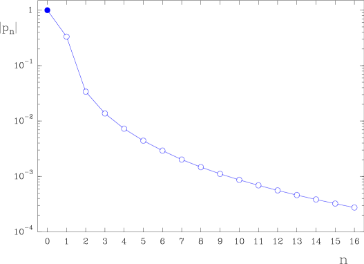
Figure 1: The first 16 coefficients in the perturbation series for the plaquette. Filled symbols show positive coefficients, empty symbols show negative coefficients. Errors are smaller than the symbols.

Unfortunately the series converges rather slowly, and simply truncating the sum at 16 loops does not give a good estimate of the complete sum. As can be seen from the graph, the dependence of the coefficients on $n$ is quite smooth, so one possible approach is to fit a curve to the known coefficients and use this to estimate the $p_{n}$ for higher $n$. This was the approach we used in [9]. The new coefficients agree very well with the predictions made in [9] when only 10 loops were available. Even at 16 loops we do not yet see signs of the series diverging, it still looks like a series with a finite radius of convergence. This suggests that the crossover region between the strong coupling and weak coupling regions is still having a strong influence on the series, as discussed in [9]. Motivated by this behaviour in the perturbative series, the possibility that there is a third-order phase transition in this region was recently examined in [10].

2.3 Boosted Perturbation Theory

It is well-known that perturbation theory in the lattice coupling $g^{2}$ converges slowly. The explanation is that the $\Lambda_{QCD}$ parameter of the bare lattice coupling $g^{2}$ is surprisingly small, $\Lambda_{lat}=0.035\Lambda_{\overline{MS}}$ so $g^{2}$ is not a very good expansion parameter. The remedy is to use a “boosted” coupling which has a more reasonable $\Lambda_{QCD}$. The most popular choice is $g^{2}_{\Box}\equiv{g^{2}}/{P}$ which has $\Lambda_{lat}=0.38\Lambda_{\overline{MS}}\;.$ The boosted coupling is larger than $g^{2}$, but we hope that the coefficients will now decrease faster, and that we will find a reliable answer with fewer terms in the series. If we had the conventional series to very high accuracy, transforming to the new coupling would be easy. However if we only have limited accuracy in the coefficients the transformation is numerically difficult as we are looking for small differences between large quantities. The solution to this problem is to modify stochastic perturbation theory so that it works directly with a boosted coupling.

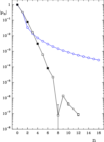
Figure 2: The boosted perturbation series (black curve, square symbols) compared with the series in the lattice coupling (blue curve, round symbols). Filled symbols show positive coefficients, open symbols show negative.

In Fig.2 we show the boosted perturbation series (from a $12^{4}$ lattice) and compare it with the conventional series. Clearly the boosted series falls off much faster. Even though we are interested in regions where the boosted coupling is 50% to 100% larger the change is worth while.

3 Perturbation Theory and Data

We are now ready to compare perturbation theory with Monte Carlo data, to see if there is any remainder which we could attribute to a condensate. If there is, how does the condensate scale, like $a^{4}$ or $a^{2}$?

In Fig.3 we show the result of summing the ordinary and the boosted perturbation series to various orders. We can see that boosted perturbation theory has a much better behaviour, it has almost ‘converged’ before we get to 12 loops, while the series in the original coupling is still changing visibly. Note that neither series shows any signs of diverging, though it is possible that if we go much further in loop number we will at some point see terms growing.

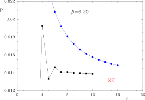
Figure 3: Convergence of the two expansions of the plaquette at $\beta=6.20$. The series in the bare lattice coupling is shown with blue circles, the series in the boosted coupling with black squares. It can be seen that the boosted series has much better apparent convergence.

The quantity which interests us here is the difference between perturbation theory and lattice Monte Carlo data, $\Delta P\equiv P_{pert}-P_{MC}$. The horizontal red line in Fig.3 shows the value of the plaquette as measured in lattice simulations. Looking at the boosted perturbation series it does seem that $P_{pert}$ is measurably larger than $P_{MC}$. It would not be as easy to estimate the gap using the unimproved series, because the result would depend heavily on extrapolated values of the $p_{n}$.

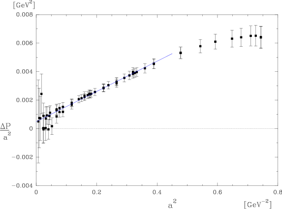
Figure 4: $\Delta P/a^{2}$ plotted against $a^{2}$, with both quantities measured in physical units. If $\Delta P$ scales like $a^{2}$ the data will be constant, if $\Delta P$ scales like $a^{4}$ the data will lie on a straight line passing through the origin.

To see whether $\Delta P$ scales like $a^{2}$ or $a^{4}$ we plot $\Delta P/a^{2}$ against $a^{2}$ in Fig.4. Most of the plaquette values are from [11], with some additional data calculated by QCDSF. If the non-perturbative contribution scales like $a^{2}$, the $\Delta P/a^{2}$ would be a constant, but if the non-perturbative contribution scales like $a^{4}$ then the data should lie on a straight line passing through the origin. We see that the data looks more like a dimension four condensate.

We can use this graph to set a bound on any dimension-two condensate. Around $a^{2}\sim 0.05{\rm GeV}^{-2}$ we see that $\left|\Delta P/a^{2}\right|<0.0015{\rm GeV}^{2}=\left(40{\rm MeV}\right)^{2}$. Since the natural scale for a dimension-two condensate is $\Lambda_{QCD}^{2}$, this is a rather tight bound.

Using eq. (2) we can find the dimension-four condensate from the slope of this graph,

$$\left\langle\frac{\alpha}{\pi}GG\right\rangle\approx 0.04(1)\;{\rm GeV}^{4}=\left(450\;{\rm MeV}\right)^{4}\;.$$ (4)

This is about the right order of magnitude, though somewhat larger than phenomenological estimates [3, 12] which tend to lie in the range $0.012$ GeV⁴ to $0.024$ GeV⁴.

4 Conclusions

Stochastic Perturbation theory gives long series for some simple quantities, allows us to test ideas that we could not look at with conventional perturbation theory. We see, for example, that boosted perturbation theory does dramatically accelerate series convergence. Although there are good reasons for expecting that perturbation theory diverges, we see no sign of this yet. Both the conventional and boosted perturbation series still look well-behaved.

The gluon condensate, found from the difference $P_{pert}-P_{MC}$, seems to be dimension four, not dimension two. The value of the gluon condensate is approximately $0.04(1)$ GeV⁴, but with large uncertainties.

References

- [1] T. Banks, R. Horsley, H. R. Rubinstein and U. Wolff, Nucl. Phys. B 190 (1981) 692.
- [2] A. Di Giacomo and G. C. Rossi, Phys. Lett. B 100 (1981) 481.
- [3] M. A. Shifman, A. I. Vainshtein and V. I. Zakharov, Nucl. Phys. B 147 (1979) 385; 448.
- [4] G. Burgio, F. Di Renzo, G. Marchesini and E. Onofri, Phys. Lett. B 422 (1998) 219.
- [5] B. Alles, M. Campostrini, A. Feo and H. Panagopoulos, Phys. Lett. B 324 (1994) 433.
- [6] A. Athenodorou, H. Panagopoulos and A. Tsapalis, Nucl. Phys. Proc. Suppl. 140 (2005) 794.
- [7] F. Di Renzo, E. Onofri and G. Marchesini, Nucl. Phys. B 457 (1995) 202.
- [8] F. Di Renzo and L. Scorzato, arXiv:hep-lat/0011067.
- [9] R. Horsley, P. E. L. Rakow and G. Schierholz, Nucl. Phys. Proc. Suppl. 106 (2002) 870.
- [10] L. Li and Y. Meurice, arXiv:hep-lat/0507034.
- [11] G. Boyd et al., Nucl. Phys. B 469 (1996) 419.
- [12] S. Narison, Phys. Lett. B 387 (1996) 162.