On the determination of low-energy constants for $\Delta{S}=1$ transitions

Abstract:

We present our preliminary results for three-point correlation functions involving the operators entering the $\Delta{S}=1$ effective Hamiltonian with an active charm quark, obtained using overlap fermions in the quenched approximation. This is the first computation carried out for valence quark masses small enough so as to permit a matching to Quenched Chiral Perturbation Theory in the $\epsilon$-regime. The commonly observed large statistical fluctuations are tamed by means of low-mode averaging techniques, combined with restrictions to individual topological sectors. We also discuss the matching of the resulting hadronic matrix elements to the effective low-energy constants for $\Delta{S}=1$ transitions. This involves (a) finite-volume corrections which can be evaluated at NLO in Quenched Chiral Perturbation Theory, and (b) the short-distance renormalization of the relevant four-quark operators in discretizations based on the overlap operator. We discuss perturbative estimates for the renormalization factors and possible strategies for their non-perturbative evaluation. Our results can be used to isolate the long-distance contributions to the $\Delta I=1/2$ rule, coming from physics effects around the intrinsic QCD scale.

PoS(LAT2005)344

1 Introduction

A satisfactory understanding of long-standing problems in kaon physics, such as the well known $\Delta{I}=1/2$ rule, has so far been elusive. In addition to final-state interactions between the two pions, the other possible origins of the $\Delta{I}=1/2$ rule are “intrinsic” long-distance QCD effects at typical energy scales of a few hundred MeV, as well as the decoupling of the charm quark from the light quark sector, owing to its large mass of around 1.3 GeV. In refs. [1, 2] we outlined a strategy to identify a mechanism for the $\Delta{I}=1/2$ rule, by separately quantifying each of the above contributions. Leaving aside final-state interactions, our strategy is implemented by computing appropriate hadronic correlation functions allowing to determine the weak low-energy constants (LECs) appearing in the effective chiral theory. Our approach is characterized by the following features:

• The use of overlap fermions [3] in computations of hadronic matrix elements of 4-quark operators mediating $\Delta{S}=1$ transitions. As described in [4] the mixing with operators of lower dimensions usually encountered with Wilson fermions is completely avoided.

• Matching to ChPT in the so-called $\epsilon$-regime of QCD, where the chiral counting rules imply that this step can be performed at NLO without the appearance of unknown LECs. Since overlap fermions preserve chiral symmetry the matching can be performed in a conceptually easy and clean manner at non-zero lattice spacing.

• Investigation of the rôle of the charm quark, keeping it as an active quark in the formulation of the effective $\Delta{S}=1$ interaction. This allows to isolate the contributions due to a large mass splitting between $m_{c}$, $m_{u}$. To this end we start with the (unphysical) situation of a mass-degenerate charm quark, $m_{c}=m_{u}$ and compute LECs as a function of $m_{c}$.

In this note we demonstrate the feasibility of our strategy in the mass-degenerate case, $m_{c}=m_{u}=m_{d}=m_{s}$, where QCD possesses an ${\rm SU(4)_{L}\times SU(4)_{R}}$ chiral symmetry. Since simulations in the $\epsilon$-regime are plagued by large statistical fluctuations [5, 6], we describe in detail how a reliable signal can be obtained for 3-point correlation functions using “low-mode averaging” (LMA) [6, 7]. Furthermore, we discuss the relations between the computed correlation functions and transition amplitudes for $K\to\pi\pi$ decays. This requires knowledge of the short-distance renormalization factors of 4-quark operators, as well as finite-volume corrections that are computed in ChPT.

2 $\Delta{S}=1$ transitions with an active charm quark

In order to make this note self-contained, we report the basic features of our approach. Ref. [1] can be consulted for full details. The decay of a neutral kaon into a pair of pions in a state with isospin $\alpha$ is described by the transition amplitude

$$T(K^{0}\to\pi\pi\big{|}_{\alpha})=iA_{\alpha}{\rm e}^{i\delta_{\alpha}},\qquad\alpha=0,\,2,$$ (1)

where $\delta_{\alpha}$ is the scattering phase shift. The experimental observation that the amplitude $A_{0}$ is significantly larger than $A_{2}$, i.e. $A_{0}/A_{2}=22.1$, is called the $\Delta{I}=1/2$ rule. Our task is the computation of correlation functions involving local operators, which can be linked to the amplitudes $A_{0}$ and $A_{2}$.

The relevant local operators are obtained via the operator product expansion of the $\Delta{S}=1$ effective weak interaction. For two generations, the effective weak Hamiltonian with an active charm quark reads

$${\cal{H}}_{\rm w}=\frac{g^{2}_{\rm{w}}}{4M_{W}^{2}}(V_{us})^{*}V_{ud}\sum_{\sigma=\pm}\left\{k_{1}^{\sigma}Q_{1}^{\sigma}+k_{2}^{\sigma}Q_{2}^{\sigma}\right\},$$ (2)

$$Q_{1}^{\pm}=\Big{\{}(\overline{s}\gamma_{\mu}P_{-}{u})(\overline{u}\gamma_{\mu}P_{-}{d})\pm(\overline{s}\gamma_{\mu}P_{-}{d})(\overline{u}\gamma_{\mu}P_{-}{u})\Big{\}}-(u\,{\to}\,c),$$ (3)

$$Q_{2}^{\pm}=(m_{u}^{2}-m_{c}^{2})\Big{\{}m_{d}({\overline{s}}P_{+}{d})+m_{s}({\overline{s}}P_{-}{d})\Big{\}},\qquad P_{\pm}={\textstyle\frac{1}{2}}(1\pm\gamma_{5}).$$ (4)

Since $Q_{2}^{\pm}$ does not contribute to the physical $K\to\pi\pi$ transition we drop it from now on. Note that the operators $Q_{1}^{+}$ and $Q_{1}^{-}$ transform according to irreducible representations of $\rm SU(4)_{L}$ of dimensions 84 and 20, respectively.

The renormalization and mixing patterns of $Q_{1}^{\pm},Q_{2}^{\pm}$ derived formally in the continuum theory are preserved on the lattice, provided that the lattice Dirac operator $D$ satisfies the Ginsparg-Wilson relation [8], and therefore an exact chiral symmetry at finite lattice spacing exists [9]. If one furthermore replaces $\psi$ by $\tilde{\psi}=(1-{{\textstyle\frac{1}{2}}}aD)\psi$, the resulting local operators in the lattice theory have simple transformation properties under the chiral symmetry. Thus, no mixing with lower-dimensional operators can occur [4].

The amplitudes $A_{0}$ and $A_{2}$ can be related to low-energy constants in an effective low-energy description of $\Delta{S}=1$ weak decays. To this end we consider the leading order effective chiral Lagrangian

$${\cal L}_{\rm E}={\textstyle\frac{1}{4}}F^{2}\,{\rm Tr}\left[(\partial_{\mu}U)\partial_{\mu}U^{\dagger}\right]-{\textstyle\frac{1}{2}}\Sigma\,{\rm Tr}\left[UM^{\dagger}{\rm e}^{i\theta/N_{\rm f}}+MU^{\dagger}{\rm e}^{-i\theta/N_{\rm f}}\right],$$ (5)

where $U\in\rm SU(4)$ denotes the Goldstone bosons, $\theta$ is the vacuum angle, and $M$ is the quark mass matrix. The LECs $F$ and $\Sigma$ denote the pion decay constant and the chiral condensate in the chiral limit. The low-energy counterpart of the $\Delta{S}=1$ effective weak Hamiltonian is obtained at lowest order in the chiral expansion as

$${\cal H}_{\rm w}^{\rm ChPT}=\frac{g^{2}_{\rm{w}}}{2M_{W}^{2}}(V_{us})^{*}V_{ud}\sum_{\sigma=\pm}g_{1}^{\sigma}\left\{[\widehat{\cal{O}}_{1}^{\sigma}]_{suud}-[\widehat{\cal{O}}_{1}^{\sigma}]_{sccd}\right\},$$ (6)

where operators containing $M$ have been neglected, and

$$[\widehat{\cal O}_{1}^{\pm}]_{\alpha\beta\gamma\delta}={\textstyle\frac{1}{4}}F^{4}\left(U\partial_{\mu}U^{\dagger}\right)_{\gamma\alpha}\left(U\partial_{\mu}U^{\dagger}\right)_{\delta\beta}+\;\hbox{projections onto irreps. of dim. 84, 20}.$$ (7)

The expression which links the LECS $g_{1}^{+}$ and $g_{1}^{-}$ to the ratio of amplitudes $A_{0}/A_{2}$ at leading order in ChPT then reads

$$\frac{A_{0}}{A_{2}}=\frac{1}{\sqrt{2}}\left(\frac{1}{2}+\frac{3}{2}\frac{g_{1}^{-}}{g_{1}^{+}}\right).$$ (8)

Finally, the LECs $g_{1}^{\pm}$ can be determined by matching suitable correlation functions in ChPT and QCD. This leads to

$${\frac{g_{1}^{-}}{g_{1}^{+}}}\,H=\frac{k_{1}^{-}(M_{W}/\Lambda)}{k_{1}^{+}(M_{W}/\Lambda)}\cdot\frac{\widehat{Z}^{-}(g_{0})}{\widehat{Z}^{+}(g_{0})}\cdot\frac{C_{1}^{-}}{C_{1}^{+}}.$$ (9)

Here, the chiral correction factor $H$ is obtained as a ratio of correlation functions of $[\widehat{\cal O}_{1}^{\pm}]$ computed in ChPT, and $C_{1}^{\pm}$ are specified in eq. (12) below. On the RHS the short-distance corrections include the Wilson coefficients $k_{1}^{\pm}$ and the renormalization factors $\widehat{Z}^{\pm}$, which relate the unrenormalized operator $(Q_{1}^{\pm})_{\rm bare}$, considered at bare coupling $g_{0}$, to the renormalization group invariant operator via

$$(Q_{1}^{\pm})_{\rm RGI}=\widehat{Z}^{\pm}(g_{0})(Q_{1}^{\pm})_{\rm bare}.$$ (10)

In the following sections we describe the evaluation of the correlation functions, the chiral correction and renormalization factors.

3 Lattice set-up in the SU(4)-symmetric case

Since preserving chiral symmetry is an essential feature of our setup, the computation of the correlation functions in Eqs. (11,12) is performed in an overlap lattice regularization. In order to match QCD to its effective low-energy description in the SU(4)-symmetric case, we start by defining suitable two- and three-point correlation functions of left-handed currents and four-quark operators in QCD, namely

$$C(x_{0}) =\sum_{\mathbf{x}}\left\langle[J_{0}(x)]_{\alpha\beta}[J_{0}(0)]_{\beta\alpha}\right\rangle\,,$$ (11)

$$C_{1}^{\pm}(x_{0},y_{0}) =\sum_{\mathbf{x},\mathbf{y}}\left\langle[J_{0}(x)]_{du}\,Q_{1}^{\pm}(0)\,[J_{0}(y)]_{us}\right\rangle\,,$$ (12)

where the non-singlet left-handed current $J_{\mu}$ is defined through

$$[J_{\mu}(x)]_{\alpha\beta}=(\bar{\psi}_{\alpha}\gamma_{\mu}P_{-}\tilde{\psi}_{\beta})(x)\,,$$ (13)

$\alpha,\beta$ are generic flavour indices, and the replacement $\psi\to\tilde{\psi}$ has been performed in the four-quark operators of Eq. (3). Recall that in the SU(4)-symmetric limit the three-point functions $C_{1}^{\pm}$ receive contributions from ”figure-8” diagrams only, since ”eye” diagrams exactly cancel due to the antisymmetrization under $(u\leftrightarrow c)$. It is also useful to define the following ratios of correlation functions, which will enter the determination of low-energy constants:

$$R_{84}(x_{0},y_{0})=\frac{C_{1}^{+}(x_{0},y_{0})}{C(x_{0})C(y_{0})}\,,~{}~{}~{}~{}~{}~{}~{}~{}~{}~{}~{}~{}R_{20}(x_{0},y_{0})=\frac{C_{1}^{-}(x_{0},y_{0})}{C(x_{0})C(y_{0})}\,,$$ (14)

$$R_{84/20}(x_{0},y_{0})=\frac{C_{1}^{+}(x_{0},y_{0})}{C_{1}^{-}(x_{0},y_{0})}\,.$$ (15)

Far enough from the location of the source operators, all these ratios are expected to exhibit plateaux that can be fitted to a constant, which can then be used as input in the matching procedure to Chiral Perturbation Theory.

At low quark masses the numerical computation of correlation functions is usually hampered by the presence of large statistical fluctuations. The latter can be understood by considering the expression of the quark propagator in terms of eigenmodes of the Neuberger-Dirac operator $D$, viz

$$S(x,y)=\frac{1}{V}\sum_{k}\frac{\eta_{k}(x)\otimes\eta_{k}(y)^{\dagger}}{\bar{\lambda}_{k}+m}\,,$$ (16)

with $\bar{\lambda}_{k}=(1-{\textstyle\frac{1}{2}}\bar{a}m)\lambda_{k}$ and $D\eta_{k}=\lambda_{k}\eta_{k}$. In the regime $m\lesssim(\Sigma V)^{-1}$, which allows a matching to Chiral Perturbation Theory in the $\epsilon$-regime, the low-lying spectrum of $D_{m}=(1-{\textstyle\frac{1}{2}}\bar{a}m)D+m$ is discrete with $\Delta\lambda\approx 1/\Sigma V$, and sizeable contributions to correlation functions come from a few low modes. Large statistical fluctuations can be traced back to “bumpy” structures in the wavefunctions of these modes [12, 6].

In order to treat this problem we use low-mode averaging (LMA) introduced in [6]. The technique proceeds by treating explicitly the contribution to left-handed quark propagators coming from a few lowest-lying modes of $D$. To be specific, we split propagators as

$$S(x,y)=\sum_{k=1}^{n_{\rm low}}\frac{e_{k}(x)\otimes e_{k}(y)^{\dagger}}{\alpha_{k}}+S^{h}(x,y)\,,$$ (17)

where $S^{h}$ is the propagator in the orthogonal complement of the subspace spanned by the $n_{\rm low}$ lowest modes, $e_{k}=P_{\sigma}u_{k}+P_{-\sigma}DP_{\sigma}u_{k}$, $-\sigma$ being the chirality where $D$ possesses zero modes (if any), and $u_{k}$ is an approximate eigenmode of $D_{m}^{\dagger}D_{m}$:

$$P_{\sigma}D_{m}^{\dagger}D_{m}P_{\sigma}u_{k}=\alpha_{k}u_{k}+r_{k}\,,~{}~{}~{}~{}~{}~{}~{}~{}~{}~{}(u_{k},r_{l})=0~{}~{}~{}\forall k,l\,.$$ (18)

After inserting the RHS of Eq. (17) in the expressions for the correlation functions $C$ and $C_{1}^{\pm}$, they can be split as

$$C=C^{ll}+C^{hl}+C^{hh}\,,$$ (19)

$$C^{\pm}_{1}=C^{\pm;llll}_{1}+C^{\pm;lllh}_{1}+C^{\pm;llhh}_{1}+C^{\pm;lhhh}_{1}+C^{\pm;hhhh}_{1}\,,$$ (20)

where $l$ and $h$ denote the number of “light” and “heavy” parts of the quark propagator, respectively. Since the “light” part of $S(x,y)$ is available by construction $\forall x,y$, it is possible to exploit translational invariance to sample the all-$l$ contributions over many different source points. Furthermore, as explained in [6], by performing $n_{\rm low}$ additional inversions of the Dirac operator it is also possible to extend this to the mixed contribution $C^{hl}$. It is easy to check that the same applies to the $hlll$ contribution to $C_{1}^{\pm}$, as well as to part of the $hhll$ one. As already shown by the exploratory study in [11], the application of this technique with $n_{\rm low}\sim 20$ suffices to obtain a signal for three-point functions at values of the quark mass of interest in view of matching to $\epsilon$-regime Chiral Perturbation Theory results.

4 Correlation functions in the $\epsilon$ and $p$-regimes

Our simulation parameters are summarized in Table 1. The simulations for lattice A are those reported in [1], while lattices B and C are new results. The statistics of lattice C is currently being increased. The results quoted for lattices B and C have to be considered preliminary.

Lattice	$\beta$	$L/a$	$T/a$	$n_{\rm low}$	$L[{\rm fm}]$	$~{}~{}~{}~{}~{}~{}~{}~{}~{}~{}~{}~{}~{}~{}~{}~{}~{}~{}~{}~{}~{}~{}~{}~{}~{}~{}~{}am$	# cfgs
A	5.8485	12	30	5	1.49	0.040,0.053,0.066,0.078,0.092	638
B	5.8485	12	32	20	1.49	0.003,0.005,0.007,0.040	681
C	5.8485	16	32	20	1.99	0.002,0.003,0.020,0.030,0.040,0.060	$\sim 350$

Table 1: Simulation parameters for the runs discussed in the text. The mass values in italics are those corresponding to the $\epsilon$-regime. The statistics indicated for lattice C refers to the number of configurations for masses in the $\epsilon$-regime; for $p$-regime masses the statistics is roughly half of the indicated figure.

Our main aim is to fit to constants the plateaux in the ratios of correlation functions in Eqs. (14,15). For quark masses in the $p$-regime the procedure is straightforward, and our statistics allows quite precise results for the different ratios. An example for $R_{84/20}$ in the $p$-regime is shown in Fig. 1. It also shows the effect of LMA on correlation functions at typical $p$-regime masses.

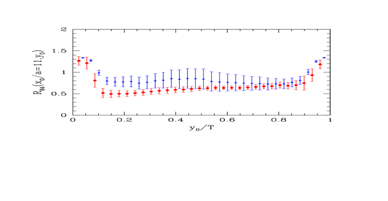
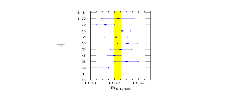
Figure 1: Left: The ratio $R_{84}$ for $am=0.020$, lattice C. The points indicated by circles (triangles) have been obtained with(out) LMA. Right: Weighted average over $|\nu|$ (solid band) of the ratio $R_{84/20}$ for $am=0.003$, lattice C.

In the $\epsilon$-regime topology plays a special rôle [13], and correlation functions are given within fixed topological sectors. Therefore we proceed by computing the quantities of interest at fixed value $|\nu|$ of the (absolute value of the) topological charge, and then perform a weighted average over $|\nu|$. In order to have large enough statistics within each sector, and taking into account the expected distribution of topological charges, we impose a bound on the largest value of $|\nu|$ entering the average ($|\nu|\leq 8$ on lattice B and $|\nu|\leq 10$ on lattice C). Furthermore, following the observation that the signal-to-noise ratio in the sectors with lowest $|\nu|$ is poor, for the largest volume (lattice C) we also impose a lower bound $|\nu|\geq 2$. This procedure is illustrated in Fig. 1. In the $\epsilon$-regime we find no signal at all for the relevant observables if LMA is not implemented. Indeed, to our knowledge, these are the first results for three-point functions obtained at quark masses in the $\epsilon$-regime.

Our most interesting results are those for the mass dependence of the different ratios. They are summarized in Fig. 2, where we put together the $p$-regime results for our three lattices and the $\epsilon$-regime results in our larger volume. Three features worth mentioning are: Firstly, the mass dependence is remarkably smooth. In particular, there is no strong mass dependence of $R_{84}$ for very small quark masses. Notice, however, that finite volume corrections have to be taken into account for the $\epsilon$-regime points (see below). Secondly, our results point towards a moderate volume dependence at quark masses corresponding to pseudoscalar meson masses around or below the kaon mass. As far as $R_{84}$ is concerned, this was already observed in [14]. Thirdly, the direct comparison of the different results at $am=0.040$ shows that the effect of LMA with an adequate number of low modes is far from negligible even at moderately large values of the pseudoscalar meson mass.

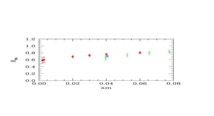
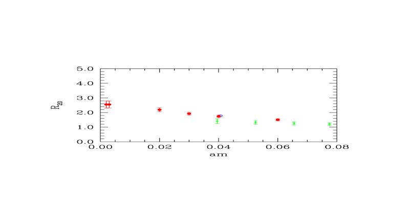
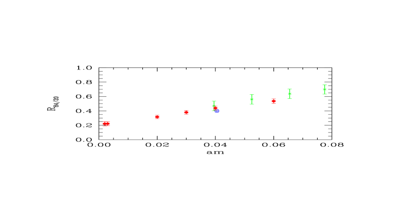
Figure 2: Mass dependence of the ratios $R_{84}$, $R_{20}$ and $R_{84/20}$ for lattices A (crosses), B (empty circles) and C (full circles). Results for lattice C are preliminary. The points at $am=0.040$ have been slightly displaced to improve visibility.

5 Renormalization factors for 4-quark operators

The renormalization factors $\widehat{Z}^{\pm}(g_{0})$ of eq. (10) are scale and scheme independent. For a particular renormalization scheme $X$ they can be decomposed according to

$$\widehat{Z}^{\pm}(g_{0})=c_{X}^{\pm}(\mu/\Lambda)\,Z_{X}^{\pm}(g_{0},a\mu),$$ (21)

where $\mu$ denotes the renormalization scale, and the coefficients $c_{X}^{\pm}$ are given by

$$c_{X}^{\pm}(\mu/\Lambda)=(2b_{0}\bar{g}^{2}(\mu))^{\gamma_{\pm;0}/(2b_{0})}\,\exp\left\{-\int_{0}^{\bar{g}(\mu)}dg\left[\frac{\gamma_{\pm}^{X}(g)}{\beta(g)}+\frac{\gamma_{\pm;0}}{{b_{0}}g}\right]\right\}.$$ (22)

The anomalous dimensions $\gamma_{\pm}^{X}$ are known in perturbation theory to two loops for several schemes. For discretizations based on the Neuberger-Dirac operator, the renormalization factors $\widehat{Z}_{X}(g_{0},a\mu)$ have been computed for $X=\rm RI/MOM$ in perturbation theory at one loop in ref. [4]. Thus, the perturbative renormalization of suitable ratios of 4-quark operators defined for overlap fermions and the RI/MOM scheme is

$$\frac{Z^{-}_{\rm RI}(g_{0},a\mu)}{Z^{+}_{\rm RI}(g_{0},a\mu)}=1+\frac{g_{0}^{2}}{16\pi^{2}}\left\{12\ln(4\mu{a})-2(B_{\rm S}-B_{\rm V})\right\}+{\rm O}(g_{0}^{4})$$ (23)

$$\frac{Z^{+}_{\rm RI}(g_{0},a\mu)}{Z_{\rm{A;RI}}^{2}(g_{0})}=1-\frac{g_{0}^{2}}{16\pi^{2}}\left\{4\ln(4\mu{a})-\frac{2}{3}(B_{\rm S}-B_{\rm V})\right\}+{\rm O}(g_{0}^{4})$$ (24)

$$\frac{Z^{-}_{\rm RI}(g_{0},a\mu)}{Z_{\rm{A;RI}}^{2}(g_{0})}=1+\frac{g_{0}^{2}}{16\pi^{2}}\left\{8\ln(4\mu{a})-\frac{4}{3}(B_{\rm S}-B_{\rm V})\right\}+{\rm O}(g_{0}^{4}).$$ (25)

The coefficients $B_{\rm S}$ and $B_{\rm V}$ are listed in Table 1 of [4]. In addition to 4-quark operators, we have also considered the renormalization of the axial current. Eqs. (24) and (25) then serve to renormalize the corresponding $B$-parameters of the operators $Q_{1}^{\pm}$. The RGI matrix elements are obtained by combining the above renormalization factors with the coefficients $c_{\rm RI}^{\pm}$.

Perturbation theory in the bare coupling $g_{0}^{2}$ is known to have bad convergence properties. The aim of “mean-field improvement” [15] is to factor out unphysical tadpole contributions in the perturbative expansion, by a rescaling of the link variable, $U_{\mu}(x)\to U_{\mu}(x)/u_{0}$. For the Neuberger-Dirac operator defined by

$$D_{\rm N}=\frac{\rho}{a}\left(1-A(A^{\dagger}{A})^{-1/2}\right),\qquad\rho=1+s,\quad|s|<1,\quad A=1+s-aD_{\rm w},$$ (26)

the corresponding rescaling of the quark field is given by $\psi\to\sqrt{(\rho/\tilde{\rho})}\psi,~{}\tilde{\rho}=(\rho-4)u_{0}+4$. For the renormalization factor $Z_{{\cal{O}}_{n}}=1+g_{0}^{2}z_{{\cal{O}}_{n}}^{(1)}+{\rm O}(g_{0}^{4})$ of an $n$-quark operator ${\cal{O}}_{n}$, the mean-field improved version reads

$$Z_{{\cal{O}}_{n}}^{\rm mfi}=\Big{(}\frac{\rho}{\tilde{\rho}}\Big{)}^{n/2}\left\{1+\tilde{g}^{2}\left[z_{{\cal{O}}_{n}}^{(1)}-\frac{n}{2}\frac{\rho-4}{\rho}u_{0}^{(1)}\right]\right\},\quad\tilde{g}^{2}\equiv\frac{g_{0}^{2}}{\langle u_{0}^{4}\rangle},$$ (27)

where $u_{0}=1+u_{0}^{(1)}g_{0}^{2}+\ldots$. When applied to our set of operators, it is immediately clear that the contributions from the prefactor $({\rho}/{\tilde{\rho}})$ as well as those proportional to $u_{0}^{(1)}$ drop out in ratios like $Z^{-}/Z^{+}$ and $Z^{\pm}/Z_{\rm A}^{2}$. Mean-field improvement of the expressions in eqs. (23)–(25) is thus simply accomplished by replacing the bare coupling $g_{0}^{2}$ by the “continuum-like” coupling $\tilde{g}^{2}$.

For a reliable determination of operator matrix elements, the use of non-perturbative estimates for renormalization factors is to be preferred. The Schrödinger functional (SF) offers a general framework for non-perturbative renormalization of QCD at all scales [16]. However, the construction of SF boundary conditions consistent with the Ginsparg-Wilson relation is quite involved [17]. In ref. [18] it was therefore proposed to introduce an intermediate Wilson-type regularization which drops out in the final result. As an example we now discuss the renormalization factor $Z^{+}/Z_{\rm A}^{2}$, which is required for the $B$-parameter $B_{\rm K}$. The desired factor relates the $B$-parameter $B_{\rm K}^{\rm ov}(g_{0})$ computed using overlap fermions, to its RGI counterpart $\widehat{B}_{\rm K}$. After introducing an intermediate regularization based, for instance, on twisted mass QCD [19], it can be written as

$$\frac{\widehat{Z}^{+}_{\rm ov}}{Z_{\rm A;ov}^{2}}(g_{0})\equiv\frac{\widehat{B}_{K}}{B_{K}^{\rm ov}(g_{0})}=\frac{\widehat{B}_{K}}{B_{K}^{\rm tm}(g_{0}^{\prime})}\cdot\frac{B_{K}^{\rm tm}(g_{0}^{\prime})}{B_{K}^{\rm ov}(g_{0})}=\left[\lim_{g_{0}^{\prime}\to 0}\frac{\widehat{Z}^{+}_{\rm tm}(g_{0}^{\prime})}{Z_{\rm A;tm}^{2}(g_{0}^{\prime})}\cdot B_{K}^{\rm tm}(g_{0}^{\prime})\right]\cdot\frac{1}{B_{K}^{\rm ov}(g_{0})},$$ (28)

where the superscripts “ov” and “tm” on the unrenormalized $B$-parameters refer to overlap and twisted mass fermions, respectively. The key observation is that the expression in square brackets is nothing but $B_{K}$ in the continuum limit, which, for instance, has been computed by the ALPHA Collaboration in quenched QCD [14]. Denoting the result by $\widehat{B}_{K}^{\rm ALPHA}$, the renormalization factor in eq. (28) is ${\widehat{B}_{K}^{\rm ALPHA}}/{B_{K}^{\rm ov}(g_{0})}$. Of course, in this way one cannot predict $B_{K}$ any more, since its value is used to formulate the renormalization condition. However, the procedure can be used to determine the value of $B_{K}$ in the chiral limit, $\widehat{B}_{K}^{\chi}$, in units of $\widehat{B}_{K}^{\rm ALPHA}$:

$$\widehat{B}_{K}^{\chi}=\frac{\widehat{Z}^{+}_{\rm ov}}{Z_{\rm A;ov}^{2}}(g_{0})\times B_{K}^{\chi;\rm ov}(g_{0})+{\rm O}(a^{2})=\widehat{B}_{K}^{\rm ALPHA}\times\frac{B_{K}^{\chi;\rm ov}(g_{0})}{B_{K}^{\rm ov}(g_{0})}+{\rm O}(a^{2}).$$ (29)

Note that $B_{K}^{\chi;\rm ov}(g_{0})$ can be obtained from a suitable ratio of correlators computed in the $\epsilon$-regime, in conjunction with the appropriate chiral correction factor.

	bare P.T.	MFI P.T.	non-pert.
$\widehat{Z}^{-}/\widehat{Z}^{+}$	0.525	0.582	0.58(8)
$\widehat{Z}^{+}/Z_{\rm A}^{2}$	1.242	1.193	1.20(8)
$\widehat{Z}^{-}/Z_{\rm A}^{2}$	0.657	0.705	0.73(8)

Table 2: Perturbative and non-perturbative estimates for RGI renormalization factors at $\beta=5.8485$.

We now discuss some numerical examples for perturbative and non-perturbative estimates of renormalization factors. In our simulations we use $\beta=6/g_{0}^{2}=5.8485$. For $\mu=2\,{\rm GeV}$ and $\Lambda=238\,{\rm MeV}$ [20], the perturbative expressions for the coefficients $c_{\rm RI}^{\pm}$ yield $c_{\rm RI}^{-}(\mu/\Lambda)=0.6259$ and $c_{\rm RI}^{+}(\mu/\Lambda)=1.2735$. Non-perturbative estimates for the $B$-parameters computed at the physical kaon mass in the continuum limit of quenched QCD are provided by the ALPHA collaboration [14]. The results for ratios of renormalization factors are listed in Table 2.

The entries in the table show that non-perturbative estimates for renormalization factors are remarkably close to perturbative ones. Indeed, even the differences between perturbative estimates evaluated in “bare” or “mean-field improved” perturbation theory are small, presumably since ratios of operators are considered here. This is in stark contrast to the situation encountered for simple quark bilinears, for which the deviations between perturbative and non-perturbative estimates amount to about 30% at similar values of the bare coupling [21].

6 Chiral corrections

Our strategy of determining the LECs of the $\Delta{S}=1$ weak interactions requires that the kinematical range where ChPT is applicable must be accessible to lattice simulations of QCD. The so-called $\epsilon$-expansion [22] represents a systematic low-energy description of QCD in a finite volume for arbitrarily small quark masses. It is characterized kinematically by the conditions $m\Sigma{V}\sim{\rm O}(1)$, $F_{\pi}{L}\gg 1$, where $V=L^{4}$ is the four-volume, and $m$ is the quark mass. These conditions lead to different chiral counting rules compared with the more commonly known $p$-regime. In particular, since the inverse box size counts as one unit of momentum $L^{-1}\sim{\rm O}(\epsilon)$, one infers $m\sim{\rm O}(\epsilon^{4})$ and hence $m_{\pi}\sim{\rm O}(\epsilon^{2})$. For the effective Hamiltonian ${\cal H}_{\rm w}^{\rm ChPT}$ of eq. (6) this in turn implies that no additional interaction terms are generated at ${\rm O}{(\epsilon^{2})}$. In other words, the $\epsilon$-regime allows for a NLO matching of lattice data to ChPT without the appearance of additional, unknown LECs [23].

We can now work out the chiral correction factor $H$ in eq. (9). To this end we define correlation functions of the left-handed axial current in complete analogy with the fundamental theory:

$${\cal C}^{ab}(x_{0})=\int{\rm d}^{3}x\left\langle{\cal J}^{a}_{0}(x){\cal J}^{b}_{0}(0)\right\rangle,\qquad{\cal{J}}_{\mu}^{a}\equiv{\textstyle\frac{1}{2}}F^{2}(T^{a})_{\alpha\beta}\left(U\partial_{\mu}U^{\dagger}\right)_{\beta\alpha},$$ (30)

$${[\widehat{\cal C}_{1}^{\pm}(x_{0},y_{0})]}^{ab}_{\alpha\beta\gamma\delta}=\int{\rm d}^{3}x\int{\rm d}^{3}y\left\langle{\cal J}^{a}_{0}(x)[\widehat{\cal O}_{1}^{\pm}(0)]_{\alpha\beta\gamma\delta}{\cal J}^{b}_{0}(y).\right\rangle,$$ (31)

Choosing a diagonal quark mass matrix and flavour matrices $T^{a},T^{b}$ as in eq. (D.6) of [1], one defines the chiral correction factor $H$ by

$$H\equiv\frac{\widehat{\cal{C}}_{1}^{-}(x_{0},y_{0})}{\widehat{\cal{C}}_{1}^{+}(x_{0},y_{0})}=1-2R(x_{0},y_{0}).$$ (32)

For later use we also consider the chiral corrections for $B$-parameters, i.e.

$$K^{\pm}\equiv 2\,\frac{\widehat{\cal{C}}^{{\sigma}}_{1}(x_{0},y_{0})}{\widehat{\cal{C}}(x_{0})\widehat{\cal{C}}(y_{0})}=1+{\sigma}R(x_{0},y_{0}),\qquad{\sigma}=\pm.$$ (33)

Explicit expressions are listed in section 5.3 of ref. [1]. In Fig. 2 of [1] the quantity $R$ is plotted as a function of the box size for several lattice geometries. It clearly demonstrates that chiral corrections are reasonably small for box sizes $L\geq 1.5\,{\rm fm}$ and lattice geometries with $T/L\leq 2$.

7 Synthesis, conclusions and outlook

We can now combine our results for ratios of correlation functions with the appropriate renormalization and NLO chiral correction factors. We expect that the latter are best controlled for our dataset “C”, for which $T/L=2$ and $L=2\,{\rm fm}$. The link between the ratio $g_{1}^{-}/g_{1}^{+}$ and the correlation functions is given in eq. (9), while individual values for $g_{1}^{+}$ are obtained from

$$g_{1}^{+}K^{+}=k_{1}^{+}(M_{W}/\Lambda)\frac{\widehat{Z}^{+}(g_{0})}{Z_{\rm A}^{2}(g_{0})}\cdot\frac{4}{3}B_{K}^{\chi;\rm ov}(g_{0}),$$ (34)

and similarly for $g_{1}^{-}$. The LECs $g_{1}^{\pm}$ are then related to the amplitudes $A_{0},\,A_{2}$ via LO ChPT.

Our preliminary results for these amplitudes in the SU(4)-symmetric theory indicate a severe mismatch with experiment: roughly speaking, our value for $A_{0}$ is too small by a factor 2, while $A_{2}$ comes out a factor 2 too large. This produces an estimate for $A_{0}/A_{2}$ which is four times smaller than the one expected from the experimentally observed $\Delta{I}=1/2$ rule. On the other hand, this is a factor 4 larger than the naive large-$N_{\rm c}$ limit, and does thus move in the right direction compared with this case.

However, it would be premature to conclude that the $\Delta{I}=1/2$ rule is generated by the decoupling of the charm quark, since the amplitude $A_{2}$ is insensitive to the charm mass, yet its experimental value is not reproduced either in our calculation. Other possibilities for the observed mismatch are uncontrolled finite-volume corrections, quenching effects, or even the breakdown of LO ChPT when relating the LECs to the transition amplitudes. Our future work will thus concentrate on corroborating our results in the $\epsilon$-regime, as well as incorporating the effects of a non-degenerate charm quark mass. In this context we shall investigate alternative choices of correlators, which are saturated with zero modes [24].

Our calculations were performed on PC clusters at DESY Hamburg, CILEA and the Univer- sity of Valencia, as well as on the IBM Regatta at FZ Jülich. We thank all these institutions and the University of Milano-Bicocca for their support.

References

- [1] L. Giusti, P. Hernández, M. Laine, P. Weisz and H. Wittig, JHEP 11 (2004) 016 [hep-lat/0407007].
- [2] P. Hernández and M. Laine, JHEP 09 (2004) 018 [hep-ph/0407086].
- [3] H. Neuberger, Phys. Lett. B417 (1998) 141 [hep-lat/9707022]; ibid. B427 (1998) 353 [hep-lat/9801031].
- [4] S. Capitani and L. Giusti, Phys. Rev. D64 (2001) 014506 [hep-lat/0011070].
- [5] W. Bietenholz, T. Chiarappa, K. Jansen, K.I. Nagai and S. Shcheredin, JHEP 02 (2004) 023 [hep-lat/0311012].
- [6] L. Giusti, P. Hernández, M. Laine, P. Weisz and H. Wittig, JHEP 04 (2004) 013 [hep-lat/0402002].
- [7] T. DeGrand and S. Schaefer, Comput. Phys. Commun. 159 (2004) 185 [hep-lat/0401011].
- [8] P. H. Ginsparg and K. G. Wilson, Phys. Rev. D25 (1982) 2649.
- [9] M. Lüscher, Phys. Lett. B 428 (1998) 342 [hep-lat/9802011].
- [10] L. Giusti, C. Hoelbling, M. Lüscher and H. Wittig, Comput. Phys. Commun. 153 (2003) 31 [hep-lat/0212012].
- [11] L. Giusti, P. Hernández, M. Laine, C. Pena, P. Weisz, J. Wennekers and H. Wittig, Nucl. Phys. B (Proc. Suppl.) 140 (2005) 417 [hep-lat/0409031].
- [12] L. Giusti, M. Lüscher, P. Weisz and H. Wittig, JHEP 11 (2003) 023 [hep-lat/0309189].
- [13] H. Leutwyler and A. Smilga, Phys. Rev. D 46 (1992) 5607.
- [14] P. Dimopoulos, J. Heitger, C. Pena, S. Sint and A. Vladikas, Nucl. Phys. B (Proc. Suppl.) 140 (2005) 362 [hep-lat/0409026]; P. Dimopoulos, J. Heitger, C. Pena, S. Sint and A. Vladikas, in preparation; M. Guagnelli, J. Heitger, C. Pena, S. Sint and A. Vladikas, hep-lat/0505002; F. Palombi, C. Pena and S. Sint, hep-lat/0505003.
- [15] G.P. Lepage and P.B. Mackenzie, Phys. Rev. D48 (1993) 2250 [hep-lat/9209022].
- [16] K. Jansen et al., Phys. Lett. B372 (1996) 275 [hep-lat/9512009].
- [17] Y. Taniguchi, hep-lat/0412024.
- [18] P. Hernández, K. Jansen, L. Lellouch and H. Wittig, JHEP 07 (2001) 018 [hep-lat/0106011].
- [19] R. Frezzotti, P.A. Grassi, S. Sint and P. Weisz, JHEP 08 (2001) 058 [hep-lat/0101001].
- [20] S. Capitani, M. Lüscher, R. Sommer and H. Wittig Nucl. Phys. B544 (1999) 669 [hep-lat/9810063].
- [21] J. Wennekers and H. Wittig, JHEP 09 (2005) 059 [hep-lat/0507026].
- [22] J. Gasser and H. Leutwyler, Phys. Lett. B188 (1987) 477; Nucl. Phys. B307 (1988) 763.
- [23] P. Hernández and M. Laine, JHEP 01, 063 (2003) [hep-lat/0212014].
- [24] L. Giusti, P. Hernández, M. Laine, P. Weisz and H. Wittig, JHEP 01 (2004) 003 [hep-lat/0312012].