Bound state spectrum in the finite volume

Abstract:

The signature of bound state formation on the lattice is of particular interest in this talk. In the finite volume, where all states have discrete energies, it is rather hard to distinguish between a bound state and a scattering state if the bound state were close to threshold, i.e. like a “loosely bound state”. To study bound states in the finite volume, we calculate the positronium spectroscopy in the Higgs phase of $U(1)$ gauge dynamics, where the photon is massive and then massive photons give rise to the short-ranged interparticle force. We try to identify bound state formation on the basis of the Lüscher’s finite size method, which suggests specific volume dependences of the energy gap/shift from the threshold energy for either bound states or scattering states.

PoS(LAT2005)061

1 Introduction

Recently, a series of hadronic resonances have been discovered in various experiments [1]. However, some of newly discovered states have unusual properties, which are not well understood from the viewpoint of the conventional quark-antiquark or three-quark states. Lattice QCD can potentially answer the question whether those states are really exotic hadron states since lattice QCD spectroscopy has been progressing with steadily increasing accuracy in the past several years.

We are especially interested in some candidates of the molecular bound state: the $\Lambda$(1405) resonance as a $\overline{K}N$ bound state, the $f_{0}(980)$ and $a_{0}(980)$ resonances as bound states of $K\overline{K}$, the $X(3872)$ resonance as a weakly bound state of $D\overline{D}^{*}$ and so on. In particular, such states except for the $\Lambda$(1405) are very close to threshold so that they would be “loosely bound states” like a deuteron. In the infinite volume, the loosely bound state is well defined since there is no continuum state below threshold. However, in a finite box on the lattice, all states have discrete energies. Even worse, the lowest level of elastic scattering states appears below threshold in the case if an interaction is attractive between two-particles [2]. Therefore, it is hard to clearly distinguish between the loosely bound state and the scattering state in this sense.

In this paper, we present numerical studies of the bound state spectrum in the finite volume. As a pilot study of hadron molecular bound states, we explore the positronium spectroscopy in the Higgs phase of $U(1)$ gauge dynamics, where the photon is massive and then massive photons give rise to the short-ranged interparticle force. In this model, we can control bound state formation in variation with the strength of the interparticle force. We then consider the application of the Lüscher’s finite size method [2], which is relevant for elastic scattering of two particles with the finite range interaction, in order to identify the signature of bound state formation on the lattice in the finite volume.

2 Lüscher’s finite size method

Let us briefly review the Lüscher’s finite size method [2]. So far, several hadron scattering lengths have been successfully calculated by using this method. Especially, the $I=2$ $\pi-\pi$ channel, where the interaction is repulsive, have been intensively studied by one of authors [3].

It was shown by Lüscher that the $S$-wave scattering phase shift $\delta_{0}$ is related to the energy shift in the total energy of two particles in the center of mass system in a finite box [2]:

$$\tan\delta_{0}(p)=\frac{\pi^{3/2}\sqrt{q}}{{\cal Z}_{00}(1,q)}\;\;\;\;{\rm at}\;\;q=(Lp/2\pi)^{2}$$ (1)

where $p$ and $L$ are the relative momentum of two particles and the spacial extent, respectively. In a $L^{3}$ box with the periodic boundary, the generalized zeta function ${\cal Z}_{00}(s,q)\equiv\frac{1}{\sqrt{4\pi}}\sum_{{\bf n}\in{\bf Z}^{3}}({\bf n}^{2}-q)^{-s}$ is defined through analytic continuation in $s$. The asymptotic solution of Eq. (1) around $q=0$, which corresponds to the energy shift of the lowest level of scattering states, is given by

$$\Delta E=\sqrt{m_{A}^{2}+p^{2}}+\sqrt{m_{B}^{2}+p^{2}}-m_{A}-m_{B}=-\frac{2\pi a_{0}}{\mu L^{3}}\left[1+c_{1}\frac{a_{0}}{L}+c_{2}\left(\frac{a_{0}}{L}\right)^{2}\right]+{\cal O}(L^{-6})$$ (2)

with $c_{1}=-2.837297$ and $c_{2}=6.375183$. $\mu$ denotes the reduced mass of two-particles as $\mu=m_{A}\cdot m_{B}/(m_{A}+m_{B})$. The scattering length is defined through $a_{0}=\lim_{p\rightarrow 0}\tan\delta(p)/p$. Eq. (2) tells us that the lowest level of elastic scattering states appears below threshold on the lattice if an interaction is weakly attractive ($a_{0}>0$) between two particles. This point makes it difficult to discriminate between bound states and scattering states on the lattice. However, it is worth noting that the large $L$ expansion formula up to $O(L^{4})$ in Eq. (2) has no real solution of $a_{0}$ for the case $\Delta E<-\frac{\pi}{2|c_{1}|\mu L^{2}}$ [4], while $a_{0}$ is always (negative) real for $\Delta E>0$. A lower bound $\Delta E\geq-\frac{\pi}{2|c_{1}|\mu L^{2}}$ may be crucial to identify the observed state below threshold with whether the lowest level of scattering states or a bound state.

The question naturally arises as to how bound state formation is studied through the Lüscher’s formula since the quantum scattering theory implements bound state solutions. Indeed, another type of the asymptotic solution of Eq. (1) around $q=-\infty$, which was found by Seattle group [5], represents a solution of bound states. Intuitively, non-vanishing negative energy gap $\Delta E$ in the infinite volume implies that a bound state is formed between two particles. This indicates that $q=-\infty$ in the limit of $L\rightarrow\infty$ is responsible for bound state formation. According to Ref. [6], an exponentially convergent expression of the the zeta function is given for negative $q$

$${\cal Z}_{00}(1,q)=-\pi^{3/2}\sqrt{-q}+\sum_{{\bf n}\in{\bf Z^{3}}}{}^{\prime}\frac{\pi^{1/2}}{2\sqrt{\bf n^{2}}}e^{-2\pi\sqrt{-q{\bf n^{2}}}},$$ (3)

where $\sum^{\prime}_{{\bf n}\in{\bf Z}^{3}}$ means the summation without ${\bf n}=(0,0,0)$. Suppose that $p^{2}$ approaches $-\gamma^{2}<0$ (real $\gamma$) as $L\rightarrow\infty$, Eq. (1) leads to

$$\cot\delta_{0}(p)=i\;\;\;{\rm at}\;\;q=-\infty$$ (4)

in the infinite volume limit. This is certainly interpreted as bound state formation because the $S$-matrix $S={\rm e}^{2i\delta_{0}(p)}=\frac{\cot\delta_{0}(p)+i}{\cot\delta_{0}(p)-i}$ has a pole at $p^{2}=-\gamma^{2}$. Therefore, for the bound state, one can derive the large $L$ expansion formula around $q=-\infty$ from Eq. (1) [5]:

$$\Delta E=-\frac{\gamma^{2}}{2\mu}\left[1+\frac{12}{\gamma L}\frac{1}{1-2\gamma(p\cot\delta_{0})^{\prime}}e^{-\gamma L}+{\cal O}(e^{-2\gamma L})\right]$$ (5)

where $(p\cot\delta_{0})^{\prime}=\frac{d}{dp^{2}}(p\cot\delta_{0})|_{p^{2}=-\gamma^{2}}$. An $L$-independent term $-\frac{\gamma^{2}}{2\mu}$ corresponds to the binding energy in the infinite volume limit. We can learn from Eq. (5) that “loosely bound state” is supposed to receive the larger finite volume correction than that of “tightly bound state” since the expansion parameter is scaled by $\gamma$, which is associated with the binding energy.

3 Compact Scalar QED

To explore the signature of bound state formation on the lattice, we consider a bound state (positronium) between an electron and a positron in the compact QED with scalar matter:

$$S_{\rm SQED}[U,\Phi,\Psi]=S_{\rm AH}[U,\Phi]+\sum_{\rm sites}\overline{\Psi}_{x}D_{\rm W}[U]_{x,y}\Psi_{y}$$ (6)

which is the compact $U(1)$ gauge theory coupled to both scalar matter (Higgs) fields $\Phi$ and fermion (electron) fields $\Psi$. The action of “$U(1)$ gauge + Higgs” part is described by the compact $U(1)$-Higgs model:

$$S_{\rm AH}[U,\Phi]=-\beta\sum_{\rm plaq.}\Re\{U_{x,\mu\nu}\}-h\sum_{\rm link}\Re\{\Phi^{\ast}_{x}U_{x,\mu}\Phi_{x+{\mu}}\},$$ (7)

where the constraint $|\Phi_{x}|=1$ is imposed. In this study, we treat the fermion fields in the quenched approximation. We also consider the $q$-charged fermion by replacing $U(1)$ link fields as

$$U_{x,\mu}\longrightarrow U^{q}_{x,\mu}=\Pi_{i=1}^{q}U_{x,\mu}$$ (8)

in the Wilson-Dirac operator $D_{\rm W}$.

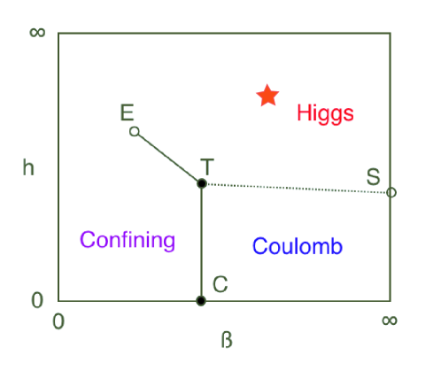
Figure 1: Schematic phase diagram of the compact $U(1)$-Higgs model in the fixed modulus case. A star mark represents our simulation point as $(\beta,h)=(2.0,\;0.6)$.

Fig.1 shows the schematic phase diagram of the compact $U(1)$-Higgs model. There are three phases: the confinement phase, the Coulomb phase and the Higgs phase. The open symbols and filled symbols represent the second-order phase transition points (E: the end point $\{\beta,h\}=\{0.8485(8),0.5260(9)\}$ [7] and S: the 4-dim XY model phase transition) and the first-order phase transition points (T: the tricritical point $\{\beta,h\}\sim\{1,0.36\}$ and C: the pure compact $U(1)$ phase transition $\beta_{c}\simeq 1$). The lines ET and TC represent the first order line. The line TS corresponds to the Coulomb-Higgs transition, of which the order is somewhat controversial in the literature because of the large finite size effect. In this study, we have fixed $\beta=2.0$ and $h=0.6$ (the Higgs phase) where massive photons give rise to the short-ranged interparticle force. In the tree level, the vacuum expectation value of the Higgs field and the photon mass are interpreted as $\langle\phi_{\rm higgs}\rangle\sim a^{-1}\sqrt{h}$ and $M_{\rm photon}\sim a^{-1}\sqrt{h/\beta}$ respectively.

4 Numerical results

We perform numerical simulations for positronium spectra (${}^{1}S_{0}$ and ${}^{3}S_{1}$ states) in the Higgs phase of $U(1)$ gauge dynamics on $L^{3}\times 24$ lattices with several spatial sizes, $L=8$, 10, 12, 16, 20, 24. Two-point functions of ${}^{1}S_{0}$ and ${}^{3}S_{1}$ states are constructed from the bilinear pseudo-scalar operator $\overline{\Psi}_{x}\gamma_{5}\Psi_{x}$ and vector operator $\overline{\Psi}_{x}\gamma_{\mu}\Psi_{x}$ respectively. To evaluate a threshold energy, we also calculate the electron mass in the Landau gauge.

Figs. 2 show masses of ${}^{1}S_{0}$ and ${}^{3}S_{1}$ positronium states as functions of the electron mass. The certain energy gap from the threshold energy appears in simulations with charge-four electron fields. It is natural to expect that higher charged electrons provide the larger energy gap since the interparticle force is proportional to (charge $q$)². For $q=4$, the hyperfine mass splitting of positronium is also clearly observed.

The volume dependences of energy gaps at $aM_{\rm electron}\simeq 0.5$ are shown in Figs. 3. All data points in the right panel ($q=4$) are clearly below the lower bound for the asymptotic solution of the scattering state. The volume dependence is drastically changed around $L\simeq 12-16$. Data for the larger lattice sizes are well fitted by the form inspired by the asymptotic solution of the bound state, Eq. (5). The energy gaps for either ${}^{1}S_{0}$ or ${}^{3}S_{1}$ states should remain finite in the infinite volume limit. Therefore, bound states of electron-positron are certainly formed in simulations with charge-four electrons even in the Higgs phase, where interparticle forces are short-ranged.

On the other hand, an upward tendency of the $L$ dependence is observed as spatial size $L$ increases in the right panel ($q=3$). However, all data points are located near the lower bound for the asymptotic solution of the scattering state. We also remark that the $L$ dependence seems to become opposite around $L\simeq 20-24$. These observations suggest that the observed states are unlikely the lowest level of elastic scattering states, rather likely a “loosely bound state”. However, to make firm conclusions on this, more detailed study and also the data for larger $L$ are required.

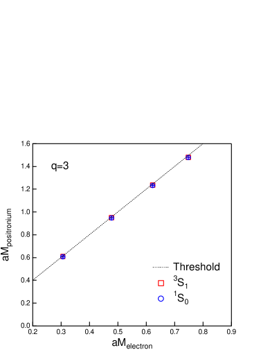
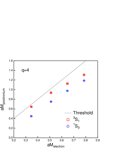
Figure 2: Masses of ${}^{3}S_{1}$ and ${}^{1}S_{0}$ positronium states as functions of the electron mass. The left (right) panel corresponds to results with charge-three (four) electrons. The dotted lines represent the threshold energy, which is evaluated by $2\times aM_{\rm electron}$.

5 Summary

We explored the signature of bound state formation in positronium spectra (${}^{1}S_{0}$ and ${}^{3}S_{1}$ states) in compact scalar QED model, where the short-range interaction between electron and positron can be realized as in the Higgs phase. In the case of highly charged electrons ($q=4$), the energy levels of both ${}^{1}S_{0}$ and ${}^{3}S_{1}$ are found to be far below threshold, while electron-positron states with the lower charged electron ($q\leq 3$) appear slightly below, but close to threshold. For $q=4$, we found a specific volume dependence of an energy gap between the total energy of electron-positron states and the threshold energy, which is well described by the asymptotic solution of the Lüscher’s formula for a bound state. More detail analysis, which includes the sensitivity test of mass spectrum with respect to spatial boundary conditions and the examination by the volume dependence of spectral weights, is now under way to investigate the formation of “loosely bound state” in the finite volume.

Acknowledgement

Thanks to RIKEN, Brookhaven National Laboratory and the U.S. DOE for providing the facilities essential for the completion of this work.

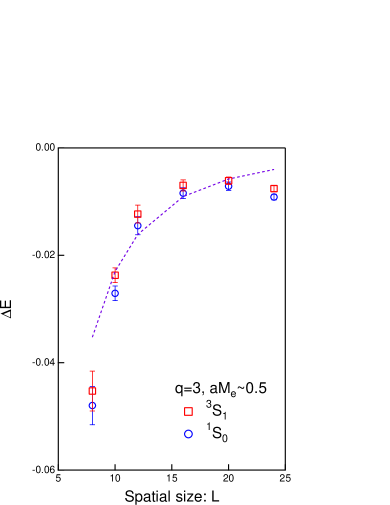
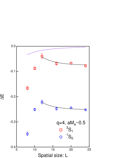
Figure 3: Mass gaps from the threshold energy as functions of spatial lattice size $L$ in lattice units. Dashed lines represent a lower bound for the asymptotic solution of the scattering state, which is given in the text. Solid curves in the right panel ($q=4$) are fits of the form $\Delta E_{L}=\Delta E_{\infty}+\frac{a}{L}e^{-bL}$, which is inspired by the asymptotic solution of the Lüscher’s formula for the bound state [5].

References

- [1] See, e.g., E. Klempt, hep-ph/0404270 and references therein.
- [2] M. Lüscher, Commun. Math. Phys. 104 (1986) 177; Nucl. Phys. B 354 (1991) 531.
- [3] T. Yamazaki et al. [CP-PACS Collaboration], Phys. Rev. D 70 (2004) 074513 . S. Aoki et al. [CP-PACS Collaboration], Phys. Rev. D 71 (2005) 094504 .
- [4] K. Yokokawa, S. Sasaki, A. Hayashigaki and T. Hatsuda, hep-lat/0509189.
- [5] S. R. Beane, P. F. Bedaque, A. Parreno and M. J. Savage, Phys. Lett. B 585 (2004) 106.
- [6] E. Elizalde, Commun. Math. Phys. 198 (1998) 83 .
- [7] J. L. Alonso et al., Phys. Lett. B 296 (1992) 154 ; Nucl. Phys. B 405 (1993) 574 .