Disconnected Loops with Twisted Mass Lattice QCD

Abstract:

We give a general introduction and discussion of the issues involved in using the twisted mass formulation of lattice fermions in the context of disconnected loop calculations, including a short orientation on the present experimental situation for nucleon strange quark form factors. A prototype calculation of the disconnected part of the nucleon scalar form factor is described.

PoS(LAT2005)039

1 Disconnected tmLQCD Calculations

Twisted mass fermions have great potential in extending lattice QCD calculations to smaller quark masses. It is essentially a chiral-flavor rotation of the mass term in the Wilson action for a quark doublet. It does not suffer from the quenched “exceptional configuration” problem because of the suppression of unphysical small quark mass eigenvalues[1]. In addition, $O(a)$ improvement is often automatic in many quantities[2]. Although twisted mass fermions are beginning to be used in phenomenological studies[3], their use in the context of lattice disconnected loop calculations is still in the initial stages. Our goal is to make realistic calculations of experimental observables, especially nucleon strange form factors. Previously, we have used Wilson fermions in our disconnected calculations[4]. The improved behavior of small quark eigenvalues in the twisted formulation changes our previous computational strategy considerably. We will discuss our computational approach below, after a brief review of the current experimental situation on strange form factors.

2 Experiments on Strange Quark Form Factors

The current experimental situation on low momentum transfer measurements of nucleon strange form factors from HAPPEX[5], A4[6], SAMPLE[7] is nicely summarized in Fig. 1 below, taken from the second paper in Ref.[5]. (Additional experimental measurements are also underway[8].) It shows a simultaneous plot of the bands in $G_{E}(q^{2}$), $G_{M}(q^{2}$) picked out by various linear combinations measured. These measurements are deduced from parity-violating asymmetry experiments done in elastic electron-proton scattering. The $95\%$ confidence region of these 4 experiments is indicated by the oval, giving small $G_{E}$, positive $G_{M}$ values. Two lattice results are indicated on the figure, listed as references 21 and 22. The reference 21 result[4] came from fitting our quenched lattice data with two chiral perturbation theory models; a “no $\eta^{\prime}$” model, and a “maximal $\eta^{\prime}$” model. The “no $\eta^{\prime}$” model is more realistic, and predicts small, positive $G_{E}$, $G_{M}$ values, in apparent agreement with experiment. Although our lattice results agree with experiment, it is clear that we must simulate at smaller quark masses to connect more confidently to the chiral models. Thus, we turn to the twisted mass formulation, which promises a deeper penetration of the chiral region.

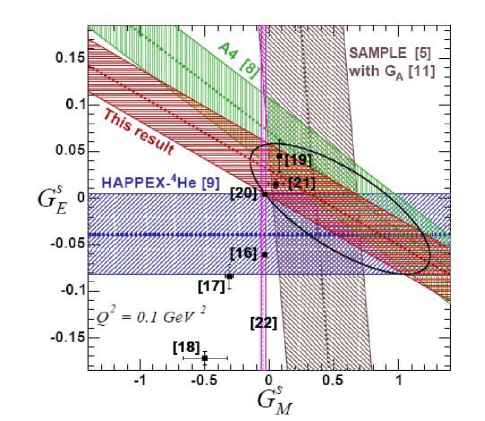
Figure 1: The experimental situation for the simultaneous measurement of the strange electric and magnetic form factors at small four-momentum transfer. Figure taken from the second paper in Ref. 5

3 Twisted Mass Eigenvalues

An illustrative eigenvalue spectrum, where we zoom in on the eigenvalues near the origin, on a small $8^{3}\times 16$ lattice with $\beta=6.0$ is shown in Fig. 2. These are actually harmonic Ritz values of the eigenvalue spectrum of the preconditioned even/odd matrix, run at $\kappa=0.1567,\mu=0.03$, which corresponds to maximal twist as determined in Ref.[9]. The harmonic Ritz values are approximate eigenvalues. The spectrum has essentially no small eigenvalues. This is in the context of the spectrum of harmonic Ritz values (a total of 140 shown) seen in Fig. 3 extending from -25 to 25 on the imaginary axis, and from 0 to 50 on the real axis. Also, one sees a symmetric pairing of up/down quark eigenvalues as one reflects across the real axis. We see these same phenomena occuring on larger lattices.

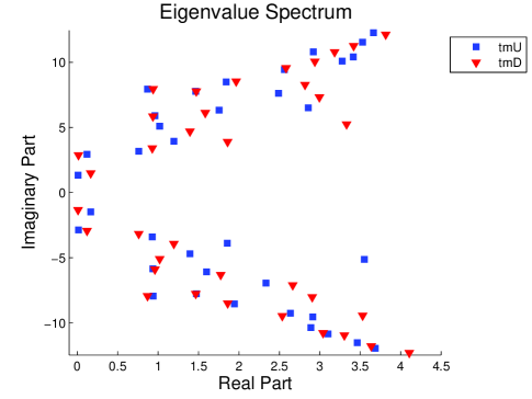
Figure 2: A selection near the origin of the even/odd preconditioned twisted mass quark eigenvalues of a small $8^{3}\times 16$ lattice.

4 tmLQCD and Perturbative Subtraction

The basic method we use to extract the subtle signals in the lattice simulation of disconnected quantities is stochastic noise projection. That is, we invert the tmWilson matrix with Z(2) noise vectors placed at every color, Dirac, and space-time position. Within this context, one of the crucial techniques we previously used in our Wilson disconnected diagram evaluations was perturbative subtraction. The perturbative evaluation of Wilson matrix elements mimics the iterative numerical evaluation, and allows a subtraction of the noise from $Z(2)$ source noise vectors. This allows a better signal to be extracted for a given number of input noise vectors, and can be used as long as one restores the perturbative signal extracted along with the noise. We tested perturbative subtraction on tmLQCD on a $20^{3}\times 32$ lattice with $\kappa=0.1567,\mu=0.03$ (about the strange quark mass). Fig. 4 shows the zero momentum time sliced disconnected signal for the imaginary part of the third component of the conserved vector current, $J_{3}(t)$, for the first 16 time positions in the lattice. We found that the method has very little effect on the extracted signal. We ran 50 noise loops for this quantity on a single configuration. The Liverpool/Münster/Zeuthen/Hamburg/Berlin group claims a better result with Gaussian noise[10]. We will soon explore this option as well.

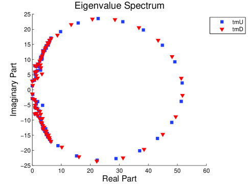
Figure 3: An illustration of the full set of even/odd preconditioned twisted mass quark eigenvalues on a small $8^{3}\times 16$ lattice.

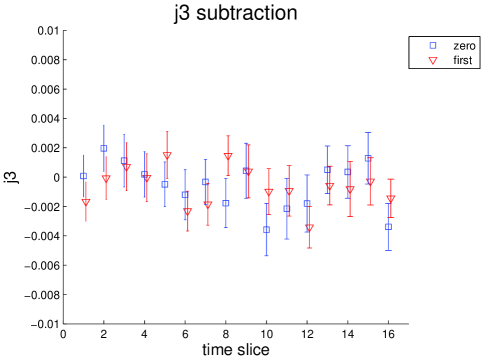
Figure 4: Illustration of the effect of perturbative subtraction on the real part of the $J_{3}$ twisted mass current loops for time positions 1 through 16 on a $20^{3}\times 32$ lattice. ”Zero” means without subtraction, ”first” means subtracted to order $\kappa^{4}$ in the perturbative series. Corresponding data points displaced slightly.

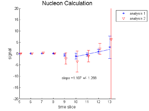
Figure 5: The blue bursts and associated error bars represent an analysis using Eq. (5.3) on 135 configurations. The red triangles and error bars are from a similar analysis, using a loop background of 20 time steps, corresponding to a fixed time upper limit in Eq. (5.3).

5 Prototype Scalar Disconnected Calculation

In order to investigate the issues arising in extracting disconnected signals in this new context, we have performed a small simulation on a $20^{3}\times 32$ lattice, at $\kappa=0.1567,\mu=0.03$, with twisted mass fermions. We use unimproved Wilson gauge fields and periodic spatial, Dirichlet time boundary conditions on the fermion fields. In addition, we ran deflated GMRES-DR(40,10)[11] (the Krylov subspace is 40, the number of deflated eigenvectors is 10.), which we find to be adequate for our needs, and GMRES-Proj[12] to use the deflated eigenvectors in solving other right hand sides. We have studied in particular the zero momentum scalar matrix element, $S=<\bar{\psi}\psi>$, in the presence of a nucleon. The quantity that we form is

$$R_{N}(t,t^{\prime})=\frac{G_{N}^{3}(t,t^{\prime})}{G_{N}^{2}(t)},$$ (1)

where $G_{N}^{3}(t,t^{\prime})$ is the three-point function for the zero momentum scalar insertion, and $G_{N}^{2}(t)$ is the two-point function for the unpolarized nucleon. The three point function is formed as

$$G_{N}^{3}(t,t^{\prime})=<G_{N}^{2}(t)S(t^{\prime})>-<G_{N}^{2}(t)><S(t^{\prime})>,$$ (2)

where $<\dots>$ denotes a gauge field average and $S(t^{\prime})$ is the raw disconnected scalar loop (we have not applied a renormalization factor). We compute the quantity,

$$R_{N}(t)=\sum_{t^{\prime}=source}^{t}R_{N}(t,t^{\prime})\longrightarrow const+G_{S}^{dis}(0),$$ (3)

which gives the disconnected part of the scalar form factor, $G_{S}^{dis}(0)$, at zero momentum. Our results (“analysis 1”) for this quantity on 135 configurations with a single noise per configuration are shown in Fig. 5. We use a zero-momentum nucleon wall source at time step 4 for the two point function. We do not attempt perturbative subtraction because of our finding, in the previous section, that this helps little. The quantity $R_{N}(t)$ is plotted as a function of the final nucleon and scalar loop position, $t$. In addition, we show another analysis (“analysis 2”) in which the upper limit in Eq.(3) is not $t$, but fixed at 20 background time steps. We are looking for a linear signal in $t$; the first analysis yields smaller error bars. The value yielded by the 10-13 time step fit is $G_{S}^{dis}(0)\approx 1.1\pm 1.3$. Although our error bar is large, the sign and magnitude of our result is consistent with expectations[4].

6 Acknowledgements

This work was supported in part by the National Science Foundation under grant 0310573 and by the Natural Sciences and Engineering Research Council of Canada. The calculations were done on the high performance cluster at Baylor University.

References

- [1] R. Frezzotti, P. A. Grassi, S. Sint and P. Weisz, JHEP 0108, 058 (2001).
- [2] R. Frezzotti and G. C. Rossi, JHEP 0408, 007 (2004).
- [3] For a very recent example with references to the literature, see Jansen et al., hep-lat/0507032.
- [4] R. Lewis, W. Wilcox, and R. M. Woloshyn, Phys. Rev. D67, 013003 (2003).
- [5] HAPPEX Collaboration, JLAB-PHY-05-312 (nucl-ex/0506010) and JLAB-PHY-05-313 (nucl-ex/0506011).
- [6] F. E. Maas et al., Phys. Rev. Lett. 94, 152001 (2005).
- [7] D. T. Spayde et al., Phys. Lett. B583, 79 (2004).
- [8] D. S. Armstrong et al., Phys. Rev. Lett. 95, 092001 (2005).
- [9] A. M. Abdel-Rehim, R. Lewis and R. M. Woloshyn, Phys. Rev. D71, 094505 (2005).
- [10] F. Farchioni et al., PoS(LAT2005)033.
- [11] R. B. Morgan, SIAM J. Sci. Comput. 24, 20 (2002).
- [12] R. B. Morgan and W. Wilcox, math-ph/0405053.