Abstract

We present results for the light quark masses obtained from a lattice QCD simulation with $N_{f}=2$ degenerate Wilson dynamical quark flavours. The sea quark masses of our lattice, of spacing $a\simeq 0.06$ fm, are relatively heavy, i.e., they cover the range corresponding to $0.60\lesssim M_{P}/M_{V}\lesssim 0.75$. After implementing the non-perturbative RI-MOM method to renormalise quark masses, we obtain $m_{ud}^{\overline{\rm{MS}}}(2\,{\rm GeV})=4.3\pm 0.4^{+1.1}_{-0}~{}\,{\rm MeV}$, and $m_{s}^{\overline{\rm{MS}}}(2\,{\rm GeV})=101\pm 8^{+25}_{-0}~{}\,{\rm MeV}$, which are about $15$% larger than they would be if renormalised perturbatively. In addition, we show that the above results are compatible with those obtained in a quenched simulation with a similar lattice.

1 Introduction

An accurate determination of quark masses is highly important for both theoretical studies of flavour physics and particle physics phenomenology. Within the quenched approximation ($N_{f}=0$), lattice QCD calculations reached a few percent accuracy, so that the error due to the use of quenched approximation became the main source of uncertainty. To examine the effects of the inclusion of the sea quarks several lattice results with either $N_{f}=2$ or $N_{f}=3$ dynamical quarks have recently been reported  [1, 2, 3, 4, 5, 6, 7, 8, 9]. Many of them seem to indicate that the unquenching lowers the physical values of light quark masses. For example, the strange quark mass, which in the quenched approximation is about $m_{s}^{\overline{\rm{MS}}}(2\,{\rm GeV})\simeq 100$ MeV, becomes $m_{s}^{\overline{\rm{MS}}}(2\,{\rm GeV})\simeq 85\div 90$ MeV when $N_{f}=2$ dynamical quarks are included [2, 3], and even smaller with $N_{f}=3$, namely $m_{s}^{\overline{\rm{MS}}}(2\,{\rm GeV})\simeq 75\div 80$ MeV [6, 7].

The accuracy of the results obtained from simulations with $N_{f}\neq 0$, however, is still limited by several systematic uncertainties. In particular, precision quenched studies of light quark masses evidenced the importance of computing the mass renormalisation constants non-perturbatively. In almost all the studies with dynamical fermions performed so far, however, renormalisation has been made by means of one-loop boosted perturbation theory (BPT). Only very recently, non-perturbative renormalisation (NPR) has been implemented in a simulation with $N_{f}=2$ by the QCDSF collaboration. The resulting strange quark mass value is $m_{s}^{\overline{\rm{MS}}}(2\,{\rm GeV})=119\pm 9$ MeV  [8], thus larger by about $20$% than the one previously reported in ref. [3], where the same lattice action and the same vector definition of the bare quark mass have been used, but with the renormalisation constant estimated perturbatively. Recently, also the Alpha collaboration reported their value for the NPR-ed strange quark mass, $m_{s}^{\overline{\rm{MS}}}(2\,{\rm GeV})=97\pm 22$ MeV [9]. It appears that the results of both QCDSF and Alpha are consistent with their previous quenched estimates [10, 11].

In this paper we present our results for the light quark masses obtained on a $24^{3}\times 48$ lattice with $N_{f}=2$ dynamical mass-degenerate quarks, in which we implement the RI-MOM NPR method of refs. [12, 13]. In the numerical simulation we used the Hybrid Monte Carlo algorithm (HMC) [14, 15], and chose to work with the Wilson plaquette gauge action and the Wilson quark action at $\beta=5.8$. The corresponding lattice spacing is $a\simeq 0.06$ fm, and the spatial extension of our lattice is $L\simeq 1.5$ fm. Gauge configurations have been generated with four different values of the sea quark mass, for which the ratio of the pseudoscalar over vector meson masses lies in the range $M_{P}/M_{V}\simeq 0.60\div 0.75$. Our final results for the average up/down and strange quark masses are

$$\begin{array}[]{ll}m_{u/d}^{\overline{\rm{MS}}}(2\,{\rm GeV})=4.3(4)(^{+1.1}_{-0})~{}\,{\rm MeV}\\ m_{s}^{\overline{\rm{MS}}}(2\,{\rm GeV})=101(8)(^{+25}_{-0})~{}\,{\rm MeV}\end{array}\qquad\left(\begin{array}[]{cc}N_{f}=2\\ \mbox{RI-MOM}\end{array}\right)\,,$$ (1)

where the first error is statistical and the second systematic, the latter dominated by discretisation lattice artifacts. Our central values refer to the quark mass definition based on the use of the axial Ward identity. The above results are larger than the ones we obtain by using one-loop BPT to compute the mass renormalisation, namely

$$\begin{array}[]{ll}m_{ud}^{\overline{\rm{MS}}}(2\,{\rm GeV})=3.7(3)(^{+1.3}_{-0})\,{\rm MeV}\\ m_{s}^{\overline{\rm{MS}}}(2\,{\rm GeV})=88(7)(^{+30}_{-0})\,{\rm MeV}\end{array}\qquad\left(\begin{array}[]{cc}N_{f}=2\\ \mbox{BPT}\end{array}\right)\,.$$ (2)

The latter values agree with the $N_{f}=2$ results reported in refs. [2, 3] in which BPT renormalisation has been used, while the values in eq. (1) agree with refs. [8, 9] in which NPR has been implemented. The values given in eq. (1) can be also compared with our quenched estimate,

$$\begin{array}[]{ll}m_{ud}^{\overline{\rm{MS}}}(2\,{\rm GeV})=4.6(2)(^{+0.5}_{-0})\,{\rm MeV}\\ m_{s}^{\overline{\rm{MS}}}(2\,{\rm GeV})=106(2)(^{+12}_{-0})\,{\rm MeV}\end{array}\qquad\left(\begin{array}[]{cc}N_{f}=0\\ \mbox{RI-MOM}\end{array}\right)\,,$$ (3)

obtained on a lattice similar in size and resolution, and by employing the same Wilson quark action. We therefore conclude that, within our statistical and systematic accuracy, and with the sea quark masses used in our simulations, we do not observe any significant effect due to the presence of dynamical quarks. We plan to pursue this study by exploring lighter sea quarks.

The remainder of this paper is organised as follows: in sec. 2 we discuss the details of our numerical simulations; in sec. 3 we present the results for the meson masses and the bare quark masses, directly accessed from the simulation; in sec. 4 we provide the mass renormalisation factors, while in sec. 5 we determine the physical quark mass values; we briefly conclude in sec. 6.

2 Simulation details

In our numerical simulation we choose to work with the Wilson action

$$S_{W}=S_{g}+S_{q}\,,$$ (4)

where $S_{g}$ is the standard Wilson plaquette gauge action,

$$S_{g}={\displaystyle{\beta\over 6}}\mathop{\displaystyle\sum}_{p}\mathrm{Tr}\,U_{p}={\displaystyle{\beta\over 6}}\mathop{\displaystyle\sum}_{x,\mu\nu}\mathrm{Tr}\,[U_{x,\mu}U_{x+\hat{\mu},\nu}U_{x+\hat{\nu},\mu}^{\dagger}U_{x,\nu}^{\dagger}]\,,$$ (5)

and $N_{f}=2$ flavours of mass-degenerate dynamical quarks are included by using the Wilson action

$$S_{q}=\mathop{\displaystyle\sum}_{x,y}\bar{q}_{x}D_{xy}q_{y}=\mathop{\displaystyle\sum}_{x,y}\bar{q}_{x}\left[\delta_{xy}-\kappa\mathop{\displaystyle\sum}_{\mu}[(1-\gamma_{\mu})U_{x,\mu}\delta_{x+\hat{\mu},y}+(1+\gamma_{\mu})U_{x,\mu}^{\dagger}\delta_{x,y+\hat{\mu}}]\right]q_{y}\,,$$ (6)

with $\kappa$ being the usual hopping parameter. The simulation parameters used in this work are summarised in table 1.

	l j $\mathbf{\beta}=5.8$				$\mathbf{\beta}=5.6$
lj $\kappa_{s}$	$0.1535$	$0.1538$	$0.1540$	$0.1541$	$0.1560$	$0.1575$	$0.1580$
$L^{3}\times T$	lj $24^{3}\times 48$				$16^{3}\times 48$
lj minutes/traj.	$10$	$12$	$16$	$21$	$5.3$	$13$	$28$
lj $T_{MC}$	$2250$	$2250$	$2250$	$2250$	$2250$	$2250$	$2250$
lj $N_{conf}$	$50$	$50$	$50$	$50$	$50$	$50$	$50$
lj $\langle P\rangle$	$0.59268(3)$	$0.59312(2)$	$0.59336(3)$	$0.59341(3)$	$0.56990(6)$	$0.57248(6)$	$0.57261(6)$
$L^{3}\times T$	lj $16^{3}\times 48$
lj minutes/traj.	$3.3$	$4.4$	$4.4$	$5.6$
lj $T_{MC}$	$4500$	$4500$	$4500$	$4500$
lj $N_{conf}$	$100$	$100$	$100$	$100$
lj $\langle P\rangle$	$0.59283(3)$	$0.59314(3)$	$0.59340(3)$	$0.59345(3)$

Table 1: Run parameters for the simulations with $N_{f}=2$. From the entire ensemble of generated HMC trajectories of unit length, $T_{MC}$, we select $N_{conf}$ for the data analysis. The stopping condition in the quark matrix inversion ($D_{xy}G_{y}=B_{x}$) is $||DG-B||<10^{-15}$. $\langle P\rangle$ is the value of the average plaquette. “Minutes/traj.” refers to the time required to produce one trajectory on the APEmille machine ($128$ GFlop).

To generate the ensembles of gauge field configurations we employ the HMC algorithm [14, 15] and implement the LL-SSOR preconditioning [16]. In solving the molecular dynamics equations we use the leapfrog integration scheme. Each trajectory of unit length ($\tau=1$) is divided into $N_{\rm step}=250$ time-steps. The resulting $\delta t=\tau/N_{\rm step}=4\times 10^{-3}$ appears to be small enough to avoid large energy differences along a trajectory, thus increasing the acceptance probability. We find an acceptance probability of about $85$%. To check the reversibility along the trajectory we verify that the quantity $||U^{\dagger}U-1||$ remains unchanged at the relative level of $10^{-11}$. For the quark matrix inversion algorithm we used the BiConjugate Gradient Stabilized (BiCGStab) method [17]. The inversion rounding errors are of the order of $10^{-8}$.

To select sufficiently decorrelated configurations we studied the autocorrelation as a function of the number of trajectories $t$ by which two configurations are separated. For a given observable $A$, the autocorrelation is evaluated as

$$C^{A}(t)={\displaystyle{{\displaystyle{1\over(T_{MC}-t)}}\displaystyle{\sum_{s=1}^{T_{MC}-t}}(A_{s}-\langle A\rangle)(A_{s+t}-\langle A\rangle)\over{\displaystyle{1\over T_{MC}}}\displaystyle{\sum_{s=1}^{T_{MC}}}(A_{s}-\langle A\rangle)^{2}}}\,,$$ (7)

where $\langle A\rangle$ is the mean value of $A$ computed on the total number of trajectories $T_{MC}$ and $A_{s}$ denotes the value measured along the trajectory $s$. After examining the autocorrelation of the plaquette and of the pseudoscalar two-point correlation functions, both shown in fig. 1, we made the conservative choice to select configurations separated by $45$ trajectories. 

Figure 1: Autocorrelations of the plaquette $C^{p}(t)$ (left), and of the pseudoscalar correlation function $C^{PS}(t)$ (right), as a function of the number of trajectories $t$ used to separate consecutive configurations. For $C^{PS}(t)$ the fluctuations around zero start at about $t=30$, indicating that configurations separated by less than $30$ trajectories are correlated. The above plots refer to the run at $\beta=5.8$ ($V=24^{3}\times 48$, and $\kappa_{s}=0.1538$).

The sea quark masses used in our simulations correspond to ratios of pseudoscalar over vector meson masses covering the range $0.60\lesssim M_{P}/M_{V}\lesssim 0.75$. In our data analysis we distinguish the sea ($\kappa_{s}$) from the valence ($\kappa_{v}$) hopping parameters, where, for each value of the sea quark mass, $\kappa_{v}$ can assume any of the values listed in table 1. The main results of this paper refer to the run made at $\beta=5.8$ and $L=24$ (i.e., $L\simeq 1.5$ fm), whereas those obtained on the lattice with $L=16$ and $\beta$ either $5.8$ ($L\simeq 1$ fm) or $5.6$ ($L\simeq 1.3$ fm) are used to investigate finite volume and discretisation effects respectively.

Finally, in order to assess the effects of quenching, we also made a quenched run ($250$ configurations) at $\beta=6.2$ and $V=24^{3}\times 56$ ($L\simeq 1.6$ fm). To reproduce the values of the $N_{f}=2$ pseudoscalar meson masses, we chose in the quenched run $\kappa_{v}\in\{0.1514,0.1517,0.1519,0.1524\}$.

An important feature of the data analysis in the partially quenched case is the appropriate treatment of the statistical errors. While the results of computations of an observable $O$ on configurations with different values of $\kappa_{s}$ are statistically independent, those computed on the gauge configurations with the same $\kappa_{s}$ but different $\kappa_{v}$ are not. To account for these correlation effects we use a combination of the bootstrap and jackknife statistical methods. At fixed $\kappa_{s}$, our data are clustered into $N_{jk}$ subsets and the statistical errors on $O$ are estimated by using the jackknife method. The resulting $N_{jk}$ values at a given $\kappa_{s}$, $O_{jk}^{\kappa_{s}}$, are then considered as a set of uniformly distributed numbers. In a next step one generates $N_{b}\gg N_{jk}$ bootstrap events by taking, for each $\kappa_{s}$, one of the uniformly distributed $O_{jk}^{\kappa_{s}}$. The variance of $O$ is then estimated by

$$\sigma^{2}_{O}=(N_{jk}-1)\times\biggl{(}\langle O^{2}\rangle_{N_{b}}-\langle O\rangle_{N_{b}}^{2}\biggr{)}\,,$$ (8)

where $\langle...\rangle_{N_{b}}$ stands for the average calculated over the $N_{b}$ bootstrap events, while the factor $(N_{jk}-1)$ takes into account the jackknife correlation at fixed $\kappa_{s}$. For a comparison, we also considered the procedure adopted in ref. [2], consisting in applying the jackknife method at one specific value of $\kappa_{s}$, while keeping the data at the remaining three $\kappa_{s}$ fixed at their central values. As expected, after adding in quadrature the four variances calculated in this way, we find excellent agreement with the estimates obtained by using eq. (8).

$\kappa_{s}$	$\kappa_{v_{1}}$	$\kappa_{v_{2}}$	$M_{P}$	$M_{V}$	$m_{v12}^{\rm AWI}(a)$
$0.1535$	$0.1535$	$0.1535$	$0.262(4)$	$0.348(8)$	$0.0333(6)$
	$0.1535$	$0.1538$	$0.252(5)$	$0.341(8)$	$0.0306(6)$
	$0.1535$	$0.1540$	$0.245(5)$	$0.336(9)$	$0.0289(6)$
	$0.1535$	$0.1541$	$0.241(5)$	$0.334(9)$	$0.0280(6)$
	$0.1538$	$0.1538$	$0.241(5)$	$0.333(9)$	$0.0280(6)$
	$0.1538$	$0.1540$	$0.233(5)$	$0.329(9)$	$0.0263(6)$
	$0.1538$	$0.1541$	$0.229(5)$	$0.326(9)$	$0.0254(6)$
	$0.1540$	$0.1540$	$0.226(5)$	$0.324(9)$	$0.0246(6)$
	$0.1540$	$0.1541$	$0.222(5)$	$0.322(10)$	$0.0237(6)$
	$0.1541$	$0.1541$	$0.218(5)$	$0.319(10)$	$0.0228(6)$
$0.1538$	$0.1535$	$0.1535$	$0.258(3)$	$0.335(4)$	$0.0314(2)$
	$0.1535$	$0.1538$	$0.247(3)$	$0.328(4)$	$0.0287(2)$
	$0.1535$	$0.1540$	$0.240(3)$	$0.323(5)$	$0.0269(2)$
	$0.1535$	$0.1541$	$0.236(4)$	$0.321(5)$	$0.0261(2)$
	$0.1538$	$0.1538$	$0.236(4)$	$0.321(5)$	$0.0260(2)$
	$0.1538$	$0.1540$	$0.228(4)$	$0.316(6)$	$0.0243(2)$
	$0.1538$	$0.1541$	$0.224(4)$	$0.314(6)$	$0.0234(2)$
	$0.1540$	$0.1540$	$0.220(4)$	$0.311(6)$	$0.0226(2)$
	$0.1540$	$0.1541$	$0.216(5)$	$0.309(7)$	$0.0217(2)$
	$0.1541$	$0.1541$	$0.212(5)$	$0.306(7)$	$0.0208(2)$
$0.1540$	$0.1535$	$0.1535$	$0.258(2)$	$0.345(5)$	$0.0303(3)$
	$0.1535$	$0.1538$	$0.247(2)$	$0.338(6)$	$0.0277(3)$
	$0.1535$	$0.1540$	$0.240(3)$	$0.333(7)$	$0.0259(3)$
	$0.1535$	$0.1541$	$0.236(3)$	$0.331(7)$	$0.0250(3)$
	$0.1538$	$0.1538$	$0.236(3)$	$0.331(7)$	$0.0250(3)$
	$0.1538$	$0.1540$	$0.228(3)$	$0.326(8)$	$0.0233(3)$
	$0.1538$	$0.1541$	$0.225(3)$	$0.324(8)$	$0.0224(3)$
	$0.1540$	$0.1540$	$0.221(3)$	$0.321(9)$	$0.0215(4)$
	$0.1540$	$0.1541$	$0.217(3)$	$0.319(9)$	$0.0207(4)$
	$0.1541$	$0.1541$	$0.212(3)$	$0.316(10)$	$0.0198(4)$
$0.1541$	$0.1535$	$0.1535$	$0.234(6)$	$0.318(10)$	$0.0286(3)$
	$0.1535$	$0.1538$	$0.222(6)$	$0.311(11)$	$0.0259(3)$
	$0.1535$	$0.1540$	$0.213(6)$	$0.307(11)$	$0.0242(3)$
	$0.1535$	$0.1541$	$0.209(6)$	$0.304(11)$	$0.0233(3)$
	$0.1538$	$0.1538$	$0.209(6)$	$0.304(11)$	$0.0233(3)$
	$0.1538$	$0.1540$	$0.200(7)$	$0.300(12)$	$0.0215(3)$
	$0.1538$	$0.1541$	$0.196(7)$	$0.298(12)$	$0.0206(3)$
	$0.1540$	$0.1540$	$0.191(7)$	$0.295(12)$	$0.0198(3)$
	$0.1540$	$0.1541$	$0.187(7)$	$0.293(13)$	$0.0189(3)$
	$0.1541$	$0.1541$	$0.182(7)$	$0.291(13)$	$0.0180(4)$

Table 2: Pseudoscalar and vector meson masses, and the bare quark masses $m_{v12}^{\rm AWI}(a)=\frac{1}{2}\bigl{[}m_{v1}(a)+m_{v2}(a)\bigr{]}^{\rm AWI}$ obtained by using the axial Ward identity method (cf. eq. (10)). Results, in lattice units, refer to the simulation with $\beta=5.8$ and $V=24^{3}\times 48$. Those obtained at $\beta=5.6$ are tabulated in appendix 1.

3 Masses of light mesons and quarks

In this section we present the results for the light pseudoscalar and vector meson masses, as well as the bare quark masses, obtained from our main data-set ($\beta=5.8$, $L=24$). These quantities are extracted from the standard study of two-point correlation functions, $C_{JJ}(t)$, in which we consider both degenerate and non-degenerate valence quarks, with valence quarks either equal or different from the sea quarks. At large Euclidean time separations, $t\gg 0$, $C_{JJ}(t)$ is dominated by the lightest hadronic state and we fit it to the form:

$$C_{JJ}(t)=\sum_{\vec{x}}\langle 0|J({\vec{x}},t)J^{\dagger}(0)|0\rangle\,\stackrel{{\scriptstyle t\gg 0}}{{\longrightarrow}}\,{Z_{JJ}\over 2M_{J}}\left(e^{-M_{J}t}+\eta\,e^{-M_{J}(T-t)}\right)\,,$$ (9)

where $\eta$ is the time reversal $(t\leftrightarrow T-t)$ symmetry factor.  The pseudoscalar and vector meson masses are extracted from $C_{PP}(t)$ and $C_{VV}(t)$ respectively, by fitting in $t\in[14,23]$. The corresponding results are listed in table 2. These results are obtained by using local source operators. We checked, however, that the Jacobi smearing procedure [18] leaves the masses unchanged, although the lowest hadronic state becomes isolated earlier.

In the same table 2 we also give the results for the quark masses obtained by using the axial Ward identity (AWI) definition. More specifically, with $A_{0}(x)=\bar{q}_{v1}\gamma_{0}\gamma_{5}q_{v2}$, and $P=\bar{q}_{v1}\gamma_{5}q_{v2}$,

$${\langle\displaystyle{\sum_{\vec{x}}}\partial_{0}A_{0}(x)P^{\dagger}(0)\rangle\over\langle\displaystyle{\sum_{\vec{x}}}P(x)P^{\dagger}(0)\rangle}\,\stackrel{{\scriptstyle t\gg 0}}{{\longrightarrow}}\,\bigl{[}m_{v1}(a)+m_{v2}(a)\bigr{]}^{\rm AWI},$$ (10)

where we fit in the same interval as before, i.e., $t\in[14,23]$. Alternatively, one can use the vector Ward identity (VWI) and relate the bare quark mass to the Wilson hopping parameter as:

$$m_{v}^{\rm VWI}(a)={\displaystyle{1\over 2}}\left({\displaystyle{1\over\kappa_{v}}}-{\displaystyle{1\over\kappa_{cr}(\kappa_{s})}}\right)\,,$$ (11)

with $\kappa_{v}$ being either $\kappa_{v1}$ or $\kappa_{v2}$ (cf. table 2), and $\kappa_{cr}(\kappa_{s})$ is the critical hopping parameter for a given sea quark mass. Notice that both the $AWI$ and $VWI$ definitions of the quark mass do depend on the values of the sea quark masses. In the axial case, this dependence is provided by the ratio of two-point correlation functions of eq. (10). In the VWI definition, the dependence on the sea quark mass is given by the value of the critical hopping parameter $\kappa_{cr}(\kappa_{s})$ computed at fixed $\kappa_{s}$. We also notice that the sea quark dependence of the critical hopping parameter is numerically equivalent to the observation made in ref. [8] where such a dependence is expressed in terms of the renormalisation constants of the singlet and non-singlet scalar density.

3.1 Lattice spacing and $\kappa_{cr}(\kappa_{s})$

In order to fix the value of the lattice spacing and $\kappa_{cr}(\kappa_{s})$, we inspect the dependence of the pseudoscalar and vector meson masses on the valence and sea quark masses. The left panel of fig. 2 shows the dependence of the vector meson masses on the squared pseudoscalar ones, which suggests a simple linear fit to the form

Figure 2: Data-points that illustrate the functional dependencies discussed in eqs. (12) and  (16).

$$M_{V}(\kappa_{s},\kappa_{v_{1}},\kappa_{v_{2}})=P_{1}+P_{2}\times M_{P}^{2}(\kappa_{s},\kappa_{v_{1}},\kappa_{v_{2}})+P_{3}\times M_{P}^{2}(\kappa_{s},\kappa_{s},\kappa_{s})\,,$$ (12)

in an obvious notation, and with capital letters used to denote that the meson masses are given in lattice units. Such a fit yields $P_{3}=0.1(3)$, i.e., the sea quark dependence is very weak. We can therefore neglect it and set $P_{3}=0$. In this way we obtain $P_{1}=0.25(1)$ and $P_{2}=1.4(2)$. We then determine the lattice spacing from this fit and by using the method of the “physical lattice planes” [19]: at the intersection of our data with the physical value for the ratio $m_{K}/m_{K^{\ast}}=0.554$, we impose that $M_{K^{\ast}}$ obtained on the lattice is $M_{K^{\ast}}=am_{K^{\ast}}^{phys}$, thus obtaining

$$a^{-1}_{m_{K^{\ast}}}=3.2(1)\,{\rm GeV}\,.$$ (13)

We also estimate the value of the lattice spacing by studying the static quark potential. At each value of the sea quark mass we extract the following values of the Sommer parameter $R_{0}=r_{0}/a$ [20]:

$$\left(R_{0}\right)_{\kappa_{s}}=\{7.52(17)_{0.1535},\,7.70(9)_{0.1538},\,7.78(19)_{0.1540},\,8.10(20)_{0.1541}\}.$$ (14)

Details on this extraction can be found in appendix 2. Assuming the observed dependence of $R_{0}$ on the sea quark mass to be physical, as the lattice spacing $a$ is supposed to be independent on the sea quark mass, we linearly extrapolate the above results to the chiral limit [$R_{0}=\alpha+\beta\times M_{P}^{2}(\kappa_{s},\kappa_{s},\kappa_{s})$], ending up with $R_{0}=8.6(4)$. After setting $r_{0}=0.5$ fm, we find

$$a^{-1}_{r_{0}}=3.4(2)\,{\rm GeV}\,,$$ (15)

in good agreement with the value given in eq. (13).

Finally, for $m_{v}^{\rm VWI}$ in eq. (11) we also need $\kappa_{cr}(\kappa_{s})$. Inspired by partially quenched ChPT [21], but neglecting the chiral logs since our dynamical quarks are not light enough, we fit our data to

$$M_{P}^{2}(\kappa_{s},\kappa_{v_{1}},\kappa_{v_{2}})=Q_{1}\,m_{v}^{VWI}[1+Q_{2}\,m_{s}^{VWI}+Q_{3}\,m_{v}^{VWI}]\,,$$ (16)

and obtain $Q_{2}=-0.2(25)$ and $Q_{3}=0.4(14)$. In other words our data are not sensitive to the quadratic corrections proportional to $Q_{2}$ and $Q_{3}$, as it can be seen from the right plot in fig. 2. Very similar feature is observed if instead of $m_{v,s}^{VWI}$ we use $m_{v,s}^{AWI}$, and therefore in the following we set $Q_{2}=Q_{3}=0$. From the resulting fit to eq. (16), we get $Q_{1}=1.70(3)$ and

$$(\kappa_{cr})_{\kappa_{s}}=\left\{0.15544(7)_{0.1535},0.15537(6)_{0.1538},0.15537(5)_{0.1540},0.15503(8)_{0.1541}\right\}\,.$$ (17)

4 Quark mass renormalisation

Before discussing the strategy to identify the physical strange and the average up/down quark masses from the results obtained by using eqs. (10,11), we need to determine the corresponding multiplicative mass renormalisation constants, $Z_{m}^{AWI}(a\mu)=Z_{A}/Z_{P}(a\mu)$, and $Z_{m}^{VWI}(a\mu)=1/Z_{S}(a\mu)$. For completeness, we also present in this section the results for $Z_{V}$, $Z_{T}$ and the quark field RC $Z_{q}$.

We use the RI-MOM method [12] which we explained in great detail in a previous publication [13]. We adopt the same notation as in ref. [13] and compute the renormalisation group invariant combinations

$$Z_{\mathcal{O}}(a\mu_{0})=C_{\mathcal{O}}(a\mu_{0})\,Z_{\mathcal{O}}^{RGI}=C_{\mathcal{O}}(a\mu_{0})\,\left(Z_{\mathcal{O}}(a\mu)/C_{\mathcal{O}}(a\mu)\right)\,,$$ (18)

for the scale dependent bilinear operators, $\mathcal{O}=S,P,T$. The evolution functions $C_{\mathcal{O}}(a\mu)$, which are known in the RI-MOM scheme at the ${\rm N^{3}LO}$ for $Z_{S}$ and $Z_{P}$ [22] and at the ${\rm N^{2}LO}$ for $Z_{T}$ [23], explicitly cancel the scale dependence of the RCs, $Z_{\mathcal{O}}(a\mu)$, at the considered order in continuum perturbation theory.

In fig. 3 we plot $Z_{V,A}$, as well as $Z_{S,P,T}(a\mu_{0})$, where in eq. (18) we choose $a\mu_{0}=1$. All of them are supposed to be flat in $(a\mu)^{2}$, where $\mu$ is the initial renormalisation scale introduced in eq. (18), modulo discretisation effects. In fact, however, we see that these effects are pronounced in the case of $Z_{S}(a\mu_{0})$, which we correct for by linearly extrapolating from $1\leq(a\mu)^{2}\leq 2$, to $(a\mu)^{2}=0$.

Figure 3: Renormalisation constants in the RI-MOM scheme at the scale $a\mu_{0}=1$, computed according to eq. (18), as a function of the initial renormalisation scale $(a\mu)^{2}$. Discretisation effects $\propto(a\mu)^{2}$ are eliminated by extrapolating the data from $1\leq(a\mu)^{2}\leq 2$, to $(a\mu)^{2}=0$. Illustration is provided for the data with $\kappa_{s}=0.1538$.

Furthermore, for the RI-MOM scheme to be mass independent we extrapolate the mild sea quark dependence linearly to the chiral limit. The results are reported in table 3. By confronting the results for the RCs obtained at $\beta=5.8$ and $L=24$ with those obtained at the same $\beta$ but with $L=16$, we find that they differ by less than $5$%. Given the smallness of the physical lattice size at $L=16$ ($\sim 1$ fm), we expect finite volume effects on our estimate of the RCs to be negligible with respect to discretization errors, which are evaluated to be of the order of $10$% (see subsec. 5.1). This is expected, since the RCs encode the short distance physics while the volume finiteness affects the long distance physics.

l j $\beta$ ($N_{f}$)	$\kappa_{s}$	$Z_{q}$	$Z_{V}$	$Z_{A}$	$Z_{S}$	$Z_{P}$	$Z_{T}$
l j $5.8$ ($N_{f}=2$)	$0.1535$	$0.81(1)$	$0.70(1)$	$0.80(2)$	$0.74(1)$	$0.54(1)$	$0.78(2)$
l j	$0.1538$	$0.80(1)$	$0.70(1)$	$0.79(2)$	$0.73(2)$	$0.55(1)$	$0.77(2)$
l j	$0.1540$	$0.78(1)$	$0.67(1)$	$0.77(2)$	$0.72(1)$	$0.52(1)$	$0.75(2)$
l j	$0.1541$	$0.79(1)$	$0.69(1)$	$0.78(2)$	$0.71(2)$	$0.52(1)$	$0.77(2)$
l j	$\kappa_{cr}(\kappa_{cr})$	$0.76(1)$	$0.66(2)$	$0.76(1)$	$0.67(3)$	$0.50(2)$	$0.74(4)$
l j	N-BPT	0.75	$0.70$	$0.77$	$0.75$	$0.61$	$0.75$
l j	TI-BPT	0.72	$0.65$	$0.73$	$0.71$	$0.55$	$0.71$
l j $5.6$ ($N_{f}=2$)	$0.1560$	$0.78(2)$	$0.63(4)$	$0.78(3)$	$0.67(2)$	$0.46(1)$	$0.76(5)$
l j	$0.1575$	$0.78(2)$	$0.64(4)$	$0.77(2)$	$0.65(2)$	$0.46(1)$	$0.77(3)$
l j	$0.1580$	$0.78(1)$	$0.66(1)$	$0.78(4)$	$0.69(2)$	$0.50(1)$	$0.78(3)$
l j	$\kappa_{cr}(\kappa_{cr})$	$0.78(1)$	$0.66(1)$	$0.78(1)$	$0.67(1)$	$0.47(1)$	$0.78(2)$
l j	N-BPT	0.74	$0.67$	$0.75$	$0.73$	$0.58$	$0.73$
l j	TI-BPT	0.69	$0.62$	$0.71$	$0.69$	$0.51$	$0.68$
l j $6.2$ ($N_{f}=0$)	$-$	$0.82(1)$	$0.71(1)$	$0.80(1)$	$0.71(1)$	$0.54(1)$	$0.79(3)$
l j	N-BPT	0.78	$0.73$	$0.79$	$0.77$	$0.65$	$0.77$
l j	TI-BPT	0.72	$0.64$	$0.73$	$0.71$	$0.55$	$0.71$

Table 3: Values of the renormalisation constants in the RI-MOM scheme at the scale $\mu=1/a$ for the two partially quenched simulations at $\beta=5.8$ ($a^{-1}=3.2(1)\,{\rm GeV}$) and 5.6 ($a^{-1}=2.4(2)\,{\rm GeV}$) and for the quenched simulation at $\beta=6.2$ ($a^{-1}=3.0(1)\,{\rm GeV}$). The quoted errors are statistical only. The non-perturbatively determined RCs are confronted to their perturbative value (BPT), where “TI” and “N” stand for the two types of boosting the bare lattice coupling as discussed in the text. Definition of $Z_{q}$ is the same one as in eq. (5) of ref. [13].

For an easier comparison of the non-perturbatively and perturbatively estimated RCs, in table 3 we also give the RCs evaluated by means of $1$-loop BPT [24]. These are obtained by replacing in the one-loop expressions of ref. [25] the bare lattice coupling by a boosted one, $g_{0}^{2}\to\widetilde{g}^{2}$. We distinguish the so-called “naïve” boosting

$$\tilde{g}^{2}={g_{0}^{2}}/\langle P\rangle\,,$$ (19)

with $\langle P\rangle\$ being the average plaquette, and the so called “tadpole improved” coupling, which is defined by inverting the perturbative series of the logarithm of the plaquette, namely 

$$\ln{\langle P\rangle}=-{\displaystyle{1\over 3}}\,\tilde{g}^{2}(3.40/a)\,\left[1-(1.1905-0.2266N_{f})\,\frac{\tilde{g}^{2}(3.40/a)}{(4\pi)}\right]\,.$$ (20)

The corresponding results for the RCs are then referred to as N-BPT and TI-BPT respectively. From the results in table 3 we see that the perturbative estimates of $Z_{S,P}$ are larger than the non-perturbative ones. In other words the non-perturbatively computed $Z_{m}^{AWI}=Z_{A}/Z_{P}$ ($Z_{m}^{VWI}=1/Z_{S}$), at $\beta=5.8$, is larger by about $15$% ($6$%) than its BPT counterpart. These differences directly propagate to the lattice determination of the renormalised quark masses. As we shall see in the following this effect explains the differences between our non-perturbatively renormalised results and those obtained by the CP-PACS and JLQCD Collaborations [2, 3], where the TI-BPT has been used. Furthermore, our results agree with those obtained in refs. [8, 9], in which the non-perturbative renormalisation has been implemented.

5 Physical light quark masses

In order to determine the physical values of the light quark masses, we need to investigate the dependence of the pseudoscalar meson masses squared on the valence and sea quark masses. From the left plot in fig. 4 we see that: (i) the dependence on the valence quark mass is linear, (ii) the slopes do not depend on $\kappa_{s}$, and (iii) the intercepts do depend on $\kappa_{s}$ and they are non-zero even when the sea quark mass is sent to zero.

Figure 4: Dependence of the pseudoscalar meson masses on the valence quark masses $m_{v}^{AWI}$ (left) and of the ratios $(M_{P}^{2}-C_{0})/m_{v}^{AWI}$ (cf. eq. (21)) on the sea quark masses $m_{s}^{AWI}$. The results refer to the case of the partially quenched simulations at $\beta=5.8$.

We can therefore fit to the form

$$M_{P}^{2}(\kappa_{s},\kappa_{v_{1}},\kappa_{v_{2}})=C_{0}(\kappa_{s})+C_{1}\,m_{v}^{AWI}[1+C_{2}\,m_{s}^{AWI}+C_{3}\,m_{v}^{AWI}]\,,$$ (21)

where the valence and sea AWI quark masses are defined in eq. (10). In this notation $m_{v}^{AWI}\equiv m^{AWI}(\kappa_{s},\kappa_{v_{1}},\kappa_{v_{2}})$, and $m_{s}^{AWI}\equiv m^{AWI}(\kappa_{s},\kappa_{s},\kappa_{s})$. Obviously, the fit forms (16) and (21) differ not only in the use of differently defined quark masses (AWI vs. VWI), but also in the presence of the constant term $C_{0}(\kappa_{s})$ in eq. (21). This term accounts for the ${\cal O}(a)$-discretisation effects present in either the pseudoscalar meson masses or the AWI quark masses or in both. Clearly, discretisation effects in the pseudoscalar meson masses also affect the fit to eq. (16), i.e., the determination of the critical hopping parameters $\kappa_{cr}(\kappa_{s})$.

As before, we find that the values of the coefficients of the quadratic terms, $C_{2}$ and $C_{3}$, in eq. (21) are consistent with zero [$C_{2}=0.6(18)$, and $C_{3}=0.08(63)$], which can be also seen from the right plot in fig. 4. Therefore we may set $C_{2}=C_{3}=0$, and from the fit to eq. (21) we obtain $C_{1}=2.05(3)$, and

$$C_{0}(\kappa_{s})=\left\{0.0007(18)_{0.1535},\,0.0023(20)_{0.1538},\,0.0046(15)_{0.1540},\,-0.0039(25)_{0.1541}\right\}\,.$$ (22)

Our partially quenched estimates of the average up/down ($m_{ud}$) and of the strange ($m_{s}$) quark masses are made by substituting on the l.h.s. of eqs. (16) and (21) the physical pion and kaon masses and using the lattice spacing value given in either eq. (13) or eq. (15). In other words, to get the quark masses in physical units, we solve

$$\left(m_{\pi}^{2}\right)^{phys.}=Q_{1}\times a^{-1}\times m_{ud}\,,$$

$$\left(m_{K}^{2}\right)^{phys.}=\frac{Q_{1}}{2}\times a^{-1}\times\left(m_{s}+m_{ud}\right)\,,$$ (23)

in the VWI case, and the analogous expressions, with the coefficient $Q_{1}$ substituted by $C_{1}$, in the AWI case. Finally the bare quark masses are multiplied by the corresponding RI-MOM mass renormalisation constants computed at $\mu_{0}=1/a$, already listed in table 3.

The conversion to the reference $\overline{\rm{MS}}$ scheme, at $\mu=2\,{\rm GeV}$, is made by using the perturbative expressions known up to N³LO accuracy [22, 27], and $\Lambda_{\overline{\rm{MS}}}^{(N_{f}=2)}=0.245(16)(20)\,{\rm MeV}$ [28]. We finally obtain

$${\rm VWI} : m_{ud}^{\overline{\rm{MS}}}(2\,{\rm GeV})=5.1(4)\,{\rm MeV}\,,\quad m_{s}^{\overline{\rm{MS}}}(2\,{\rm GeV})=120(7)\,{\rm MeV}\,,$$

$${\rm AWI} : m_{ud}^{\overline{\rm{MS}}}(2\,{\rm GeV})=4.3(4)\,{\rm MeV}\,,\quad m_{s}^{\overline{\rm{MS}}}(2\,{\rm GeV})=101(8)\,{\rm MeV}\,.$$ (24)

Notice that our VWI result is in very good agreement with the value $m_{s}^{\overline{\rm{MS}}}(2\,{\rm GeV})=119(5)(8)\,{\rm MeV}$ obtained by the QCDSF-UKQCD collaboration who uses the VWI quark mass definition and the RI-MOM non-perturbative renormalisation [8]. Notice also that our AWI result agrees with the value obtained by the Alpha collaboration, $m_{s}^{\overline{\rm{MS}}}(2\,{\rm GeV})=97(22)\,{\rm MeV}$ [9].

5.1 Systematic uncertainties

• Discretisation I: From quenched studies we learned that a discrepancy between the quark mass values obtained by using two a priori equivalent definitions, namely the VWI and AWI definitions, is due to discretisation errors. Such a difference has also been observed in other lattice studies with $N_{f}=2$ [2, 3]. In particular, in ref. [2] this difference is shown to diminish as the lattice spacing is reduced so that, in the continuum limit, the quark masses defined in the two ways converge to the same (unique) value. From that study it became clear that discretisation errors are significantly larger in the VWI determination of the quark masses which is why the JLQCD collaboration choose to quote their AWI masses as final results, while the difference between the VWI and AWI results is included in the asymmetric systematic error. We follow the same procedure here and we obtain

  $$m_{ud}^{\overline{\rm{MS}}}(2\,{\rm GeV})=4.3(4)(^{+0.8}_{-0})\,{\rm MeV}\,, m_{s}^{\overline{\rm{MS}}}(2\,{\rm GeV})=101(8)(^{+19}_{-0})\,{\rm MeV}\,.$$ (25)

• Discretisation II: The results reported in eq. (5) refer to the lattice with coupling $\beta=5.8$ (and volume $24^{3}\times 48$). From our data produced at $\beta=5.6$ (see table 1) we obtain

  $$m_{ud}^{\overline{\rm{MS}}}(2\,{\rm GeV})=4.2(3)(^{+0.7}_{-0})\,{\rm MeV}\,, m_{s}^{\overline{\rm{MS}}}(2\,{\rm GeV})=101(6)(^{+18}_{-0})\,{\rm MeV}\,,$$ (26)

  thus indistinguishable from those obtained at $\beta=5.8$. This makes us more confident that the discretisation error attributed to our results in eq. (25) is realistic.

• Lattice spacing: To obtain the results quoted in eq. (25) we used the lattice spacing (13) fixed by $m_{K^{\ast}}^{phys.}$. These results would become larger by $6$% if we used $a^{-1}_{r_{0}}$ (15). We will add this difference to our final error budget.

• Renormalisation constants: As discussed in the text the determination of the mass renormalisation factors is sensitive to discretisation errors. They are especially important when the unimproved Wilson quark action is used, which is the case with our study. To check for these effects we determined $Z_{P}/Z_{S}$ by using the hadronic Ward identities (hWI) [29] (see eqs. (16,17) of ref. [13]), obtaining

  $$\left(Z_{P}/Z_{S}\right)^{\rm hWI}=0.67(1)\,.$$ (27)

  Compared to the results in table 3, where at $\beta=5.8$ we find $(Z_{P}/Z_{S})^{\rm RI-MOM}=0.75(1)$, this result is about $11$% smaller. A similar effect is seen at $\beta=5.6$. We observe that, either one attributes this effect to $Z_{P}$ or to $Z_{S}$, $(Z_{P}/Z_{S})^{\rm hWI}$ always goes in the direction of decreasing the AWI-VWI mass difference. Therefore, this $11$% uncertainty, being already enclosed in the $19$% systematic error due to the AWI-VWI mass difference, will not be added. We finally notice that the result obtained for $Z_{P}/Z_{S}$ by using the numerical stochastic perturbation theory to $4$-loops, i.e., $(Z_{P}/Z_{S})^{\rm NSPT}=0.77(1)$ [30], is more consistent with our larger NPR-ed (i.e., RI-MOM) value.

• Finite volume: Our data at $\beta=5.8$ and $16^{3}\times 48$ (see appendix 1) indicate large finite volume effects, when compared to our main data-set with $\beta=5.8$ and $24^{3}\times 48$. As an illustration we show in fig. 5 the effective mass plots obtained in the two volumes at the same value of the sea quark mass.

  Figure 5: Pseudoscalar and vector effective mass plots at two different volumes at $\beta=5.8$ and with $\kappa_{s}=0.1538$. Valence quark masses are equal to that of the sea quark. The physical volumes correspond to $(1.5~{}{\rm fm})^{3}$ and $(1~{}{\rm fm})^{3}$ respectively.

  Such a sensitivity to the finiteness of the lattice box has already been observed in ref. [31], where it was shown that, for the range of sea quark masses used in our study, finite volume effects are large at $L\simeq 1$ fm but become insignificant when working on lattices with $L\geq 1.5$ fm. We will rely on that conclusion and will assume that finite volume effects are negligible with respect to our statistical and other sources of systematic errors. For a more refined estimate of these effects calculations on lattices with larger volumes are required.

We add the above systematic errors algebraically and, as a final result, we quote

$$\begin{array}[]{ll}m_{ud}^{\overline{\rm{MS}}}(2\,{\rm GeV})=4.3\pm 0.4^{+1.1}_{-0}~{}\,{\rm MeV}\\ m_{s}^{\overline{\rm{MS}}}(2\,{\rm GeV})=101\pm 8^{+25}_{-0}~{}\,{\rm MeV}\end{array}\qquad\left(\begin{array}[]{cc}N_{f}=2\,,\quad\beta=5.8\\ \mbox{RI-MOM}\end{array}\right)\,,$$ (28)

which are the values already given in the abstract and the introduction of the present paper.

5.2 Impact of non-perturbative renormalisation and quenching effects

Before concluding this section we should compare our main results for the light quark masses quoted in eq. (28) with those obtained by evaluating the quark mass RCs using one-loop tadpole improved BPT:

$$\begin{array}[]{ll}m_{ud}^{\overline{\rm{MS}}}(2\,{\rm GeV})=3.7\pm 0.3^{+1.3}_{-0}~{}\,{\rm MeV}\\ m_{s}^{\overline{\rm{MS}}}(2\,{\rm GeV})=88\pm 7^{+30}_{-0}~{}\,{\rm MeV}\end{array}\qquad\left(\begin{array}[]{cc}N_{f}=2\,,\quad\beta=5.8\\ \mbox{TI-BPT}\end{array}\right)\,.$$ (29)

These results are in good agreement with those available in the literature obtained from lattice studies with $N_{f}=2$ in which renormalisation is implemented perturbatively, namely $m_{s}^{\overline{\rm{MS}}}(2\,{\rm GeV})=88(^{+4}_{-6})\,{\rm MeV}$ [2], and $m_{s}^{\overline{\rm{MS}}}(2\,{\rm GeV})=84.5(^{+12.0}_{-1.7})$ MeV [3]. Therefore, with Wilson-like dynamical fermions, the non-perturbative renormalisation increases the values of the quark masses.

Finally, when compared with our results obtained in the quenched simulation at $\beta=6.2$,

$$\begin{array}[]{ll}m_{ud}^{\overline{\rm{MS}}}(2\,{\rm GeV})=4.6\pm 0.2^{+0.5}_{-0}~{}\,{\rm MeV}\\ m_{s}^{\overline{\rm{MS}}}(2\,{\rm GeV})=106\pm 2^{+12}_{-0}~{}\,{\rm MeV}\end{array}\qquad\left(\begin{array}[]{cc}N_{f}=0\,,\quad\beta=6.2\\ \mbox{RI-MOM}\end{array}\right)\,,$$ (30)

on a lattice similar in size and resolution and by using the same (unimproved) Wilson quark action, we see no evidence for any effect that could be attributed to the presence of the dynamical quarks. For a clearer conclusion concerning this point one should work with lighter sea quark masses which is one of the main goals of our future simulations.

6 Conclusions

In this paper we have presented our results for the light quark masses obtained from a numerical simulation of QCD on the lattice with $N_{f}=2$ degenerate dynamical quarks, with masses covering the range $3/4\lesssim m_{q}/m_{s}^{phys}\lesssim 3/2$ (with respect to the physical strange quark mass). Our main values for the strange and for the average up/down quark masses are obtained on a lattice with spacing $a\approx 0.06$ fm and spatial volume $(1.5~{}{\rm fm})^{3}$, and by using the axial Ward identity. An important feature of our calculation is that we renormalise the quark masses non-perturbatively in the RI-MOM scheme, which is then converted to the $\overline{\rm{MS}}$ scheme by using the known $4$-loop perturbative formulae. We show that

• within our statistical accuracy and with relatively heavy dynamical quarks, our unquenched results are fully consistent with the quenched ones; 

• the non-perturbative renormalisation leads to resulting quark masses larger than those renormalised by using $1$-loop perturbation theory (even if tadpole improved);

• the systematic errors are dominated by lattice discretisation artifacts, which can be cured by implementing $\mathcal{O}(a)$-improvement and/or working with several small lattice spacings followed by an extrapolation to the continuum limit.

The finiteness of the lattice volume is expected not to be an important source of systematic errors for the sea quark masses explored in our simulation. Further decrease of the dynamical quark masses would necessitate, however, to work with larger physical lattice volumes. Our final results are given in eq. (28).

Appendix 1: Meson masses from two simulations with larger coupling ($\beta=5.6$) and smaller volume ($16^{3}\times 48$)

In this appendix we provide the reader with two sets of results. We first give our values equivalent to the ones presented in table 2 but for $\beta=5.6$. Then, for the reader to better appreciate the size of finite volume effects at $\beta=5.8$, we also tabulate the pseudoscalar and vector meson masses on the spatial volumes $16^{3}$ and $24^{3}$ in the fully unquenched situations, i.e., with $\kappa_{v}=\kappa_{s}$.

$\kappa_{s}$	$\kappa_{v_{1}}$	$\kappa_{v_{2}}$	$M_{P}$	$M_{V}$	$m_{v12}^{\rm AWI}(a)$
$0.1560$	$0.1560$	$0.1560$	$0.441(5)$	$0.541(6)$	$0.0669(4)$
	$0.1560$	$0.1575$	$0.398(6)$	$0.513(8)$	$0.0548(5)$
	$0.1560$	$0.1580$	$0.383(7)$	$0.503(8)$	$0.0509(5)$
	$0.1575$	$0.1575$	$0.351(7)$	$0.482(9)$	$0.0430(5)$
	$0.1575$	$0.1580$	$0.334(8)$	$0.471(10)$	$0.0392(6)$
	$0.1580$	$0.1580$	$0.317(9)$	$0.459(10)$	$0.0355(6)$
$0.1575$	$0.1560$	$0.1560$	$0.379(3)$	$0.456(8)$	$0.0515(4)$
	$0.1560$	$0.1575$	$0.333(4)$	$0.417(13)$	$0.0394(4)$
	$0.1560$	$0.1580$	$0.316(4)$	$0.403(16)$	$0.0355(4)$
	$0.1575$	$0.1575$	$0.280(4)$	$0.374(21)$	$0.0276(3)$
	$0.1575$	$0.1580$	$0.261(4)$	$0.357(27)$	$0.0238(3)$
	$0.1580$	$0.1580$	$0.241(4)$	$0.340(35)$	$0.0200(3)$
$0.1580$	$0.1560$	$0.1560$	$0.368(3)$	$0.468(11)$	$0.0466(4)$
	$0.1560$	$0.1575$	$0.324(5)$	$0.443(15)$	$0.0348(4)$
	$0.1560$	$0.1580$	$0.308(6)$	$0.436(18)$	$0.0311(4)$
	$0.1575$	$0.1575$	$0.271(7)$	$0.419(21)$	$0.0234(5)$
	$0.1575$	$0.1580$	$0.250(9)$	$0.419(27)$	$0.0199(5)$
	$0.1580$	$0.1580$	$0.227(11)$	$0.424(37)$	$0.0164(5)$

Table 4: Values of pseudoscalar and vector meson masses, as well as of the AWI quark masses $m_{v12}^{\rm AWI}(a)=\frac{1}{2}\bigl{[}m_{v1}(a)+m_{v2}(a)\bigr{]}^{\rm AWI}$ obtained by using eq. (10), as obtained from the simulation at $\beta=5.6$. All results are given in lattice units.

$\kappa_{s}=\kappa_{v}$	$M_{P}^{(24)}$	$M_{P}^{(16)}$	$\Delta_{P}$	$M_{V}^{(24)}$	$M_{V}^{(16)}$	$\Delta_{V}$
$0.1535$	$0.262(4)$	$0.299(6)$	$0.14(4)$	$0.348(8)$	$0.402(13)$	$0.16(5)$
$0.1538$	$0.236(4)$	$0.272(10)$	$0.15(4)$	$0.321(5)$	$0.356(17)$	$0.11(6)$
$0.1540$	$0.221(3)$	$0.257(8)$	$0.17(4)$	$0.321(9)$	$0.347(23)$	$0.08(7)$
$0.1541$	$0.182(7)$	$0.251(9)$	$0.38(4)$	$0.291(13)$	$0.328(31)$	$0.13(8)$

Table 5: Pseudoscalar and vector meson masses, in lattice units, calculated at $\beta=5.8$ on the lattices $24^{3}\times 48$ and $16^{3}\times 48$, respectively. Finite volume effects are quantified by $\Delta_{P,V}=(M_{P,V}^{(16)}-M_{P,V}^{(24)})/M_{P,V}^{(24)}$.

Appendix 2: The scale parameter $R_{0}=r_{0}/a$

To determine the Sommer scale parameter $R_{0}$ [20] we computed the static quark potential $V(R)$ which is extracted from the time dependence of the rectangular Wilson loops $W(R,t)$, where $R$ is the spatial separation between the static charges, i.e.,

$$W(R,t)={\cal C}(R)e^{-V(R)t}\,\Rightarrow\,V(R)=\lim_{t\to\infty}V_{\rm eff}(R,t)\equiv\lim_{t\to\infty}\log\left({W(R,t)\over W(R,t+1)}\right)\,.$$ (31)

Large time separations are reached after using the so-called HYP (hypercubic blocking) procedure proposed in ref. [33] which helps in improving the signal for the Wilson loops. In this way we find a stable signal for $V(R)$ for $t_{\rm fit}\in[8,13]$. At intermediate spatial separations between the static charges, we then fit the data (shown in fig. 6) to the form

$$V(R)=V_{0}+\sigma R-{e\over R}-g\delta V(R)\,,$$ (32)

where we also account for $\delta V(R)$, the perturbatively estimated discretisation correction to the Coulomb potential [34]. The Sommer scale $R_{0}$ is defined as

$$\biggl{(}R^{2}{dV(R)\over dR}\biggr{)}_{R=R_{0}}=1.65\,.$$ (33)

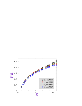
Figure 6: Static quark potential obtained from the simulation with $N_{f}=2$ at $\beta=5.8$ on the lattice $24^{3}\times 48$.

The fitting window consistent with the form (32) is found for $R\in[2,7]$ after which the statistical quality of the data for $V(R)$ rapidly deteriorates. From the fit of our data to the form (32) in that window, we obtain

$$\beta=5.8\,:\qquad\kappa_{s} = \{0.1535,\,0.1538,\,0.1540,\,0.1541\}\,,$$

$$R_{0} = \{7.52(17),\,7.70(9),\,7.78(19),\,8.10(20)\}\,,$$

$$\sqrt{\sigma} = \{0.155(4),\,0.151(2),\,0.150(4),\,0.144(4)\}\,,$$ (34)

$$e = \{0.289(10),\,0.302(5),\,0.294(7),\,0.288(13)\}\,,$$

$$V_{0} = \{0.260(7),\,0.268(3),\,0.264(5),\,0.262(9)\}\,,$$

$$g = \{0.033(14),\,0.036(9),\,0.035(7),\,0.015(15)\}\,,$$

ordered as the values of $\kappa_{s}$. Our results for $R_{0}$ obtained at the same value of $\beta$ but on the smaller volume ($16^{3}\times 48$) agree with those written in eq. (Appendix 2: The scale parameter $R_{0}=r_{0}/a$), within the statistical errors.

At $\beta=5.6$, we find stability for $t_{\rm fit}\in[3,5]$, and then from the fit to eq. (32) in $R\in[2,7]$, we have

$$\beta=5.6\,:\qquad\kappa_{s} = \{0.1560,\,0.1575,\,0.1580\}\,,$$

$$R_{0} = \{5.15(5),\,5.72(10),\,5.98(8)\}\,,$$

$$\sqrt{\sigma} = \{0.225(3),\,0.202(4),\,0.195(3)\}\,,$$ (35)

$$e = \{0.305(11),\,0.317(8),\,0.308(6)\}\,,$$

$$V_{0} = \{0.262(9),\,0.279(7),\,0.275(5)\}\,,$$

$$g = \{0.009(11),\,0.022(7),\,0.020(4)\}\,,$$

in good agreement with ref. [31].

References

• [1] P. E. L. Rakow, Nucl. Phys. Proc. Suppl.  140 (2005) 34 [hep-lat/0411036]; R. Gupta, eConf C0304052 (2003) WG503 [hep-ph/0311033]; H. Wittig, Nucl. Phys. Proc. Suppl.  119 (2003) 59 [hep-lat/0210025].
• [2] A. Ali Khan et al. [CP-PACS Collaboration], Phys. Rev. D 65 (2002) 054505 [Erratum-ibid. D 67 (2003) 059901] [hep-lat/0105015].
• [3] S. Aoki et al. [JLQCD Collaboration], Phys. Rev. D 68 (2003) 054502 [hep-lat/0212039].
• [4] Y. Namekawa et al. [CP-PACS Collaboration], Phys. Rev. D 70 (2004) 074503 [hep-lat/0404014].
• [5] C. Dawson [RBC Collaboration], Nucl. Phys. Proc. Suppl.  128 (2004) 54 [hep-lat/0310055].
• [6] T. Ishikawa et al. [CP-PACS Collaboration], Nucl. Phys. Proc. Suppl.  140 (2005) 225 [hep-lat/0409124].
• [7] C. Aubin et al. [HPQCD Collaboration], Phys. Rev. D 70 (2004) 031504 [hep-lat/0405022].
• [8] M. Gockeler et al. [QCDSF and UKQCD Collaborations], hep-ph/0409312.
• [9] M. Della Morte et al. [ALPHA Collaboration], hep-lat/0507035.
• [10] M. Gockeler et al., Phys. Rev. D 62 (2000) 054504 [hep-lat/9908005].
• [11] J. Garden et al. [ALPHA Collaboration], Nucl. Phys. B 571 (2000) 237 [hep-lat/9906013].
• [12] G. Martinelli, C. Pittori, C. T. Sachrajda, M. Testa and A. Vladikas, Nucl. Phys. B 445 (1995) 81 [hep-lat/9411010].
• [13] D. Becirevic et al., JHEP 0408 (2004) 022 [hep-lat/0401033].
• [14] S. Duane et al., Phys. Lett. B 195 (1987) 216; S. A. Gottlieb et al., Phys. Rev. D 35, 2531 (1987).
• [15] A. D. Kennedy, Nucl. Phys. Proc. Suppl.  140 (2005) 190 [hep-lat/0409167]; M. Hasenbusch, Nucl. Phys. Proc. Suppl.  129 (2004) 27 [hep-lat/0310029].
• [16] S. Fischer et al., Comput. Phys. Commun.  98 (1996) 20 [hep-lat/9602019]; A. Frommer et al., Int. J. Mod. Phys. C 5 (1994) 1073 [hep-lat/9404013].
• [17] H. van der Vost, SIAM (Soc. Ind. Appl. Math), J. Sci. Sat. Comput. 13, 631 (1992).
A. Frommer et al., Int. J. Mod. Phys. C 5 (1994) 1073 [hep-lat/9404013].
• [18] C. R. Allton et al. [UKQCD Collaboration], Phys. Rev. D 47 (1993) 5128 [hep-lat/9303009].
• [19] C. R. Allton et al., Nucl. Phys. B 489 (1997) 427 [hep-lat/9611021].
• [20] R. Sommer, Nucl. Phys. B 411 (1994) 839 [hep-lat/9310022].
• [21] C. W. Bernard and M. F. L. Golterman, Phys. Rev. D 49 (1994) 486 [hep-lat/9306005]; S. R. Sharpe, Phys. Rev. D 56 (1997) 7052 [Erratum-ibid. D 62 (2000) 099901] [hep-lat/9707018].
• [22] K. G. Chetyrkin and A. Retey, Nucl. Phys. B 583 (2000) 3 [hep-ph/9910332].
• [23] J. A. Gracey, Nucl. Phys. B 662 (2003) 247 [hep-ph/0304113].
• [24] G. P. Lepage and P. B. Mackenzie, Phys. Rev. D 48 (1993) 2250 [hep-lat/9209022].
• [25] S. Capitani, Phys. Rept.  382 (2003) 113 [hep-lat/0211036].
• [26] M. Crisafulli et al., Eur. Phys. J. C 4 (1998) 145 [hep-lat/9707025].
• [27] K. G. Chetyrkin, Phys. Lett. B 404 (1997) 161 [hep-ph/9703278]; J. A. M. Vermaseren, S. A. Larin and T. van Ritbergen, Phys. Lett. B 405 (1997) 327 [hep-ph/9703284]; T. van Ritbergen, J. A. M. Vermaseren and S. A. Larin, Phys. Lett. B 400 (1997) 379 [hep-ph/9701390]; K. G. Chetyrkin, B. A. Kniehl and M. Steinhauser, Phys. Rev. Lett.  79 (1997) 2184 [hep-ph/9706430].
• [28] M. Della Morte et al. [ALPHA Collaboration], Nucl. Phys. B 713 (2005) 378 [hep-lat/0411025]; M. Gockeler et al., hep-ph/0502212.
• [29] M. Bochicchio et al., Nucl. Phys. B 262 (1985) 331.
• [30] F. Di Renzo et al., hep-lat/0509158.
• [31] B. Orth, T. Lippert and K. Schilling, Phys. Rev. D 72 (2005) 014503 [hep-lat/0503016].
• [32] D. Becirevic, V. Lubicz and C. Tarantino [SPQcdR Collaboration], Phys. Lett. B 558 (2003) 69 [hep-lat/0208003]; D. Becirevic, V. Gimenez, V. Lubicz and G. Martinelli, Phys. Rev. D 61 (2000) 114507 [hep-lat/9909082]; D. Becirevic et al., Phys. Lett. B 444 (1998) 401 [hep-lat/9807046]; C. R. Allton, V. Gimenez, L. Giusti and F. Rapuano, Nucl. Phys. B 489 (1997) 427 [hep-lat/9611021].
• [33] A. Hasenfratz and F. Knechtli, Phys. Rev. D 64 (2001) 034504 [hep-lat/0103029].
• [34] C.B. Lang and C. Rebbi, Phys. Lett. B 115 (1982) 137.