The chiral transition in two-flavor QCD

Abstract:

QCD with $N_{f}$=2 is a specially interesting system to investigate the chiral transition. The order of the transition has still not been established. We report the results of an in-depth numerical investigation performed with staggered fermions on lattices with $L_{t}$=4 and $L_{s}$=12,16,20,24,32 and quark masses $am_{q}$ ranging from 0.01335 to 0.307036. Using finite-size techniques we compare the scaling behavior of a number of thermodynamical susceptibilities with the expectations of $O(4)$ and $O(2)$ universality classes. Clear disagreement is observed. Indications of a first order transition are found. Preliminary reports of this work were presented at past Lattice conferences.

PoS(LAT2005)158

1 Introduction

The phase transition in $N_{f}=2$ QCD ($m_{u}=m_{d}\equiv m$) can provide fundamental insight into the mechanism of confinement[1].

In the limit $m\rightarrow\infty$ the system is quenched, the deconfining transition is first order, $\langle L\rangle$ is the order parameter and $Z_{3}$ the symmetry. However the coupling to quarks breaks $Z_{3}$.

At $m\simeq 0$ the deconfining transition seems to coincide with the chiral transition. A transition line exists at intermediate values of $m$ which is defined by the maxima of a number of susceptibilities (the specific heat $C_{V}$, the susceptibility $\chi_{m}$ of the chiral condensate $\langle\bar{\psi}\psi\rangle$, the susceptibility of $\langle L\rangle$) which all coincide whithin errors (see e.g. Ref.[2]).

At $m\simeq 0$ a renormalization group analysis[3] indicates that the chiral transition is first order for $N_{f}\geq 3$, and for $N_{f}=2$ can be either first order or second order in the universality class of $O(4)$. For the latter case the transition is a crossover at $m\neq 0$, and in particular a tricritical point is expected in the $T-\mu$ plane[4] which could be observed in heavy ion collisions.

Various groups have studied this problem with Wilson[5] or staggered[6, 7, 2, 8, 9] fermions. No clear sign of discontinuities is found at least for the lattice sizes used, but no agreement either with the critical exponents of $O(4)$.

We investigate the issue using standard Kogut-Susskind fermions on lattices $4\times L_{s}^{3}$ with $L_{s}=12,16,20,24,32$ and lattice quark masses $am_{q}$ ranging from $0.01335$ to $0.307036$. In the present work we give our final results using our whole dataset collected on APEmille machines and a detailed analysis which is different in many points from the previous ones present in the literature. Preliminary reports of this work were presented at past conferences.

2 Analysis of the critical behavior

The order of a phase transition can be investigated by finite size scaling analysis. Near the critical point, for a second or a weak first order transition, the singular behavior is described by power law divergences according to universal critical exponents. The singular part of the free energy density ${\cal F}_{s}$ is a homogeneuos function of the reduced temperature $\tau\equiv 1-T/T_{c}$, the lattice quark mass $am_{q}$ and the size of the system $L_{s}$:

$${\cal F}_{s}(\tau,am_{q},L_{s})=L_{s}^{-d}{\cal F}_{s}\left(\tau L_{s}^{y_{t}},am_{q}L_{s}^{y_{h}}\right)$$ (1)

There are two independent critical exponents: the thermal $y_{t}$ and the magnetic one $y_{h}$. The other more familiar critical exponents are given by ($d=3$ is the dimensionality of the system):

$$\alpha=2-\frac{d}{y_{t}}\hskip 34.14322pt\beta=\frac{d}{y_{t}}-\frac{y_{h}}{y_{t}}\hskip 34.14322pt\gamma=2\frac{y_{h}}{y_{t}}-\frac{d}{y_{t}}\hskip 34.14322pt\delta=-\frac{y_{h}}{d-y_{h}}\hskip 34.14322pt\nu=\frac{1}{y_{t}}$$ (2)

The numerical values of the critical exponents of interest for this work are given in Table 1.

	$y_{t}$	$y_{h}$	$\nu$	$\alpha$	$\gamma$	$\beta$	$\delta$
$O(4)$	1.336(25)	2.487(3)	0.748(14)	-0.24(6)	1.479(94)	0.3837(69)	4.852(24)
$O(2)$	1.496(20)	2.485(3)	0.668(9)	-0.005(7)	1.317(38)	0.3442(20)	4.826(12)
$MF$	$3/2$	$9/4$	$2/3$	0	1	1/2	3
$1^{st}Order$	3	3	$1/3$	1	1	0	$\infty$

Table 1: Critical exponents of $O(4)$, $O(2)$, mean field and first order.

According to Eq. 1 this problem involves two scaling variables. We simplify the problem restricting the parameter space in three different ways:

1. keep $am_{q}L_{s}^{y_{h}}$ fixed while varying $L_{s}$. One must choose a fixed value for $y_{h}$ so that only one universality class at a time can be tested. Note that by chance the numerical value of $y_{h}$ is the same for $O(4)$ and $O(2)$, so in practice we can test these two critical behaviors at once. The scaling law for ${\cal F}_{s}$ is given by: ${\cal F}_{s}=L_{s}^{-d}{\cal F}_{s}\left(\tau L_{s}^{y_{t}}\right)$ where now $am_{q}$ is a function of $L_{s}$;

2. keep $\tau$ and $am_{q}$ fixed and take the limit $L_{s}\rightarrow\infty$ (finite mass scaling, Ref. [2, 8, 9]). This amounts to assume the existence of one single scale ($am_{q}$) in the problem, and no divergence of the correlation length at the transition: i.e. finite mass scaling and no finite size scaling. Eq. (1) becomes: ${\cal F}_{s}=am_{q}^{d/y_{h}}{\cal F}_{s}(\tau am_{q}^{-y_{t}/y_{h}})$ where the size of the system $L_{s}$ is not present;

3. the last possibility is to keep $\tau L_{s}^{y_{t}}$ fixed while taking $L_{s}$ much bigger than the pion correlation lenght: $aL_{s}\gg 1/m_{\pi}$. This should work better than case 2. if the correlation lenght becomes large and comparable to $L_{s}$. The free energy scaling law in this case is: ${\cal F}_{s}=am_{q}^{d/y_{h}}{\cal F}_{s}\left(\tau L_{s}^{y_{t}}\right)$.

In cases 2. and 3. we are not forced to fix $y_{h}$ so we are free to test all the critical behaviors of interest. The price for this is that we were forced to make additional approximations.

Taking appropriate derivatives we find the relevant scaling laws for the thermodynamic susceptibilities. In this work we concentrate on two of them: the specific heat $C_{V}$ and the chiral susceptibility $\chi_{m}$. Note that while the first quantity is always relevant, the second one is a good quantity only if $\langle\bar{\psi}\psi\rangle$ is the order parameter: that is certainly true for $m=0$ but may not be for $m>0$. The expected behavior for the cases listed above are:

1. $C_{V}-C_{0}=L_{s}^{\alpha/\nu}\phi_{c}(\tau L_{s}^{1/\nu})$ ; $\chi_{m}-\chi_{0}=L_{s}^{\gamma/\nu}\phi_{\chi}(\tau L_{s}^{1/\nu})$. i.e. the peaks scale as a power of $L_{s}$ and the widths as $L_{s}^{-1/\nu}$;

2. $C_{V}-C_{0}=(am_{q})^{-\alpha/\nu y_{h}}\phi_{c}(\tau(am_{q})^{-y_{t}/y_{h}})$ ; $\chi_{m}-\chi_{0}=(am_{q})^{-\gamma/\nu y_{h}}\phi_{\chi}(\tau(am_{q})^{-y_{t}/y_{h}})$. i.e. the peaks scale as a power of $am_{q}$ and the widths as $am_{q}^{y_{t}/y_{h}}$;

3. $C_{V}-C_{0}=(am_{q})^{-\alpha/\nu y_{h}}\phi_{c}(\tau L_{s}^{1/\nu})$ ; $\chi_{m}-\chi_{0}=(am_{q})^{-\gamma/\nu y_{h}}\phi_{\chi}(\tau L_{s}^{1/\nu})$. i.e. the peaks scale as a power of $am_{q}$ and the width as $L_{s}^{-1/\nu}$.

	Run1				Run2
$L_{s}$	12	16	20	32	12	16	20	32
$am_{q}$	0.153518	0.075	0.04303	0.01335	0.307036	0.15	0.08606	0.0267
# Traj.	22500	87700	14520	14500	25000	131390	16100	15100
$aL_{s}\cdot m_{\pi}$	11.9	11.0	10.0	8.9	11.3	15.8	14.8	12.4

Table 2: Run parameters for our Monte Carlo simulations. A more detailed list can be found in Ref. [1].

To test different scaling hypotheses we have performed a huge amount of Monte Carlo simulations, divided into three groups (see Table 2). The first two are called Run1 and Run2 and they satisfy the requirements of case 1., namely we have fixed $am_{q}L_{s}^{y_{h}}$ to two different values and $y_{h}$ appropriate for $O(4)$ and $O(2)$. The third group is formed by two other simulations with the following parameters: $L_{s}=16$, $am_{q}=0.01335$; $L_{s}=24$, $am_{q}=0.04444$; with $10000$ trajectories each. Simulations were made using the hybrid R algorithm sweeping a wide range of values of $\beta$ for each value of $am_{q}$. The datasets collected were analysed using the multi-histogram reweighting procedure.

3 Results

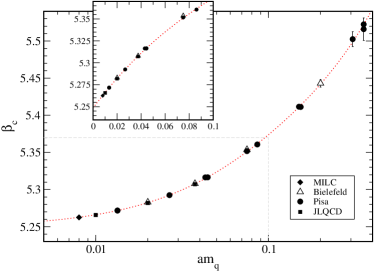
Figure 1: Pseudocritical coupling values as a function of $am_{q}$. The fit (explained in the text) has $\chi^{2}/dof=0.9$, $dof=15$. Values obtained from other collaborations are also included.

On the lattice the reduced temperature is expressed as a function of the parameters $\beta$, $am_{q}$:

$$\tau\equiv 1-\frac{T}{T_{0}}=1-\frac{a(\beta_{0},0)}{a(\beta,am_{q})}$$ (3)

where $a(\beta,am_{q})$ is the lattice spacing. Expanding $a$ in power series near $(\beta_{0},0)$ we obtain:

$$\tau\propto(\beta_{0}-\beta)+k_{m}am_{q}+k_{m^{2}}(am_{q})^{2}+k_{m\beta}am_{q}(\beta_{0}-\beta)+\cdots$$ (4)

In previous works in the literature it was assumed that $\tau\propto(\beta_{0}-\beta)$ thus neglecting the lattice spacing dependence on the lattice quark mass $am_{q}$. The terms in Eq. (4) prove to be sufficient to describe the data of our simulations. There are two different way the pseudocritical temperature could scale: $\tau_{c}=k_{\tau}L_{s}^{1/\nu}$ or $\tau_{c}=k^{\prime}_{\tau}am_{q}^{y_{t}/y_{h}}$. The expansion parameters and $k_{\tau}$ or $k^{\prime}_{\tau}$ can be obtained by fitting numerical data. The results are the following: there is no visible shift of $\tau_{c}$ varying $L_{s}$, i.e. $k_{\tau}$ is always compatible with zero; data are equally well described by all the critical behaviors expected (first order, $O(4)$, $O(2)$, MF) if one includes in the expression of $\tau_{c}$ the quadratic terms shown above; including only the linear terms the statement doesn’t change if we restrict the allowed range of $am_{q}$ (see Ref. [1]); taking $\tau_{c}\propto\beta_{0}-\beta_{c}$ does not describe the data in any mass range at our disposal for a second order while for a first order it is identical to keep only the linear mass term in Eq. (4).

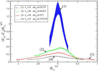
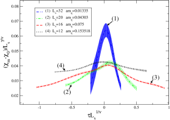
Figure 2: Scaling behavior of $C_{V}$ and $\chi_{m}$ as expected in case 1. No sign of scaling is found. This excludes a second order $O(4)$ or $O(2)$ transition. Simulations from Run1 are shown; Run2 is similar[1].

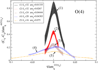
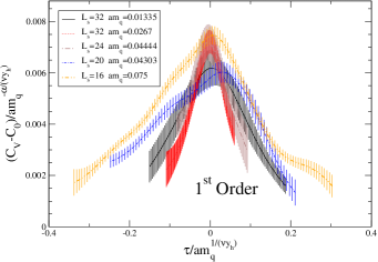
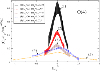
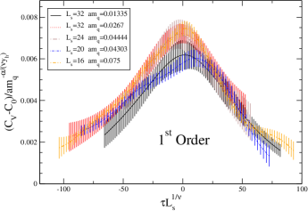
Figure 3: Scaling of $C_{V}$ according to case 2. (top) and 3. (bottom) for both $O(4)$ (left) and first order (right). Other second order behaviors are similar to the one shown.

Having fixed the parameters for the reduced temperature $\tau$ (see Fig. 1) we can next consider the scaling of $C_{V}$ and $\chi_{m}$. We first consider case 1: using data from Run1 and Run2 we can check $O(4)$ and $O(2)$ critical behaviors. If there is scaling all the curves obtained by plotting the susceptibilities divided by the appropriate power of $L_{s}$ as functions of the scaling variable $\tau L_{s}^{y_{t}}$ should collapse onto a universal scaling function. As shown in Fig. 2 no such scaling is observed for $O(4)$ ($O(2)$ is quite similar). This clearly excludes these universality classes. To check other critical behaviors we consider the scaling of cases 2. and 3. We show in Fig. 3 the analysis of $C_{V}$: similar considerations also apply to $\chi_{m}$. The second order critical behavior does not describe our data. The growth of the peaks is instead consistent with a first order. This is an indication for a first order transition. The widths of the curves seem to be described by the scaling of case 3 and not according to case 2. This means that the dependence on $L_{s}$ cannot be neglected. We have also explicitely observed consistent deviations from the scaling predicted in case 2. making simulations at two different volumes with the same $am_{q}$, see Ref. [1]. In fact this is due to the presence of two different physical scales in the problem.

One can also study the magnetic equation of state, i.e. the scaling of $\langle\bar{\psi}\psi\rangle-\langle\bar{\psi}\psi\rangle_{0}=am_{q}^{1/\delta}F(\tau/am_{q}^{1/\nu y_{h}})$ as shown in Fig. 4.

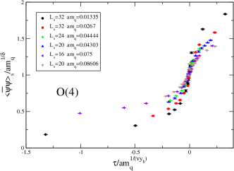
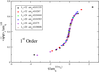
Figure 4: Scaling of $\langle\bar{\psi}\psi\rangle$ for $O(4)$ (left) and first order (right).

Also in this case the first order behavior seems to describe well the data while the second order is excluded.

We have looked for metastabilities in the time histories as required by a first order transition: no clear evidence exists up to the lattice sizes explored.

4 Conclusions and outlook

We have investigated the nature of the chiral transition in $N_{f}=2$ QCD. By using the correct definition of $\tau$ on the lattice we have shown that it is not possibile to discriminate the order of the transition by looking only at $\beta_{c}$ with the present data. Studying the critical behavior at fixed $am_{q}L_{s}^{y_{h}}$ we were able to exclude the second order universality classes, i.e. $O(4)$, $O(2)$, mean field. We found evidence for a first order transition looking at the scaling of thermodynamic susceptibilities but no clear sign of discontinuities. The magnetic equation of state also seems compatible with a first order transition. We plan to repeat the analysis at fixed $am_{q}L_{s}^{y_{h}}$ for a first order transition employing an improved action and $L_{t}=6$ to reduce possible artifacts.

References

- [1] M. D’Elia, A. Di Giacomo and C. Pica, hep-lat/0503030.
- [2] F. Karsch, Phys. Rev. D 49, 3791; F. Karsch and E. Laermann, Phys. Rev. D 50, 6954;
- [3] R. D. Pisarski and F. Wilczek, Phys. Rev. D 29, 338;
- [4] M. A. Stephanov, K. Rajagopal and E. V. Shuryak, Phys. Rev. Lett. 81 4816;
- [5] A. A. Khan et al. (CP-PACS collaboration), Phys. Rev. D 63, 034502;.
- [6] M. Fukugita, H. Mino, M. Okawa and A. Ukawa, Phys. Rev. Lett. 65, 816; Phys. Rev. D 42, 2936;
- [7] F. R. Brown, F. P. Butler, H. Chen, N. H. Christ, Z. Dong, W. Schaffer, L. I. Unger and A. Vaccarino, Phys. Rev. Lett. 65, 2491;
- [8] S. Aoki et al. (JLQCD collaboration), Phys. Rev. D 57, 3910;
- [9] C. Bernard, C. DeTar, S. Gottlieb, U. M. Heller, J. Hetrick, K. Rummukainen, R.L. Sugar and D. Toussaint, Phys.Rev. D 61, 054503;