Low-mode averaging for baryon correlation functions

Abstract:

The low-mode averaging technique is a powerful tool for reducing large fluctuations in correlation functions due to low-mode eigenvalues of the Dirac operator. In this work we propose a generalization to baryons and test our method on two-point correlation functions of left-handed nucleons, computed with quenched Neuberger fermions on a lattice with extension $L\;=\;1.5$ fm. We show that the statistical fluctuations can be reduced and the baryon signal significantly improved.

PoS(LAT2005)132

1 Introduction

It is a known fact that arbitrarily small eigenvalues of the massless Dirac operator $D$ can occur [1, 2, 3, 4, 5, 6], and that local “bumps” of the corresponding wave functions can be reflected in large fluctuations of the physical observables [6]. In particular, in the quark mass region $m\sim 1/\Sigma V$, where $V$ is the volume and $\Sigma$ is the bare quark condensate, we expect that few eigenvectors could give a substantial contribution to the observables; in that case the fluctuations can be reduced in an efficient way by applying an exact low-mode averaging procedure. By adopting the techniques developed in [7, 8], low-mode averaging has been applied to quenched meson correlation functions with Neuberger fermions, both in the $\epsilon$- and $p$-regimes [8, 9].
This technique can be generalized to a wider class of correlators; in particular this work is devoted to its application to baryon two-point functions. After clarifying the theoretical framework, we present a numerical study with quenched Neuberger fermions in the $p$-regime.

2 Low-mode averaging for baryonic two-point functions

In the following we consider a lattice of volume $V=L^{3}T$ with lattice spacing $a$ and periodic boundary conditions in all directions. We assume that fermions are discretized by using the Neuberger–Dirac operator $D$ [10], which satisfies the Ginsparg–Wilson relation [11]; this ensures that chiral symmetry is preserved at finite lattice spacing [12]. The conventions used in this work are the same as in [8], to which the reader can refer for undefined notations. We adopt the neutron interpolating field

$$N_{L}(x)=\left[\tilde{u}_{L}^{aT}(x)C\gamma_{5}\tilde{d}_{L}^{b}(x)\right]\tilde{d}_{L}^{c}(x)\epsilon^{abc},$$ (1)

where $\tilde{q}=\left(1-\frac{1}{2}\overline{a}D\right)q$ and $C$ is the charge conjugation matrix. We consider the two-point function

$$C_{N}(t)=\sum_{\vec{x}}\langle{\rm Tr}\left(N_{L}(x)\overline{N}_{L}(0)\gamma_{0}\right)\rangle,$$ (2)

where the trace is meant over the nucleon spinor indices. Following ref. [7], for each gauge configuration we can extract the first $n$ low modes of the Dirac operator and express the left–left propagator as the sum of the light and heavy parts:

$$S_{L}(x,y)=P_{-}S(x,y)P_{+}=P_{-}\left[\sum_{i=0}^{n-1}\varphi_{i}(x)\varphi_{i}^{\dagger}(y)+S^{h}(x,y)\right]P_{+},$$ (3)

where $P_{\pm}=(1\pm\gamma_{5})/2$ and

$$\varphi_{i}(x)=\frac{1}{\sqrt{\overline{\lambda_{i}}}}\left[P_{c}\psi_{i}+P_{-c}DP_{c}\psi_{i}\right](x).$$ (4)

Here, $P_{c}$ ($c=\pm$) is the projector on the chiral sector with no zero modes, and $\overline{\lambda_{i}}$, $\psi_{i}$ are respectively the approximate eigenvalues and eigenvectors of $A=P_{c}D_{m}^{\dagger}D_{m}P_{c}$, where $D_{m}$ is the massive Neuberger–Dirac operator. The use of the left-handed propagator avoids the complications due to the contribution of the zero modes to the correlation function. The baryon correlation function in eq. (2) can be split into four contributions:

$$C_{N}(t)=C_{N}^{hhh}(t)+C_{N}^{hhl}(t)+C_{N}^{hll}(t)+C_{N}^{lll}(t),$$ (5)

where $h$ ($l$) means that the heavy (light) part of the propagator is involved. The ensemble average of each contribution is translational invariant, and therefore its Monte Carlo variance can be reduced by averaging over equivalent space-time points. There are two possible contractions that contribute to the correlation function of eq. (2), and in the case of degenerate quark masses, the $lll$ part can be written as

$$C_{N}^{{lll}}(t)=\frac{1}{V}\sum_{x,y}\delta_{t,t_{x}-t_{y}}\sum_{i,j=0}^{n-1}{\rm Tr}\left[P_{+}\left(\varphi_{i}^{a}(x)\varphi_{i}^{g\;\dagger}(y)\right)^{T}C\gamma_{5}P_{-}\varphi_{j}^{b}(x)\varphi_{j}^{f\;\dagger}(y)C\gamma_{5}\right]$$ (6)

$$\sum_{k=0}^{n}{\rm Tr}\left[P_{-}\varphi_{k}^{c}(x)\varphi_{k}^{e\;\dagger}(y)\gamma_{0}\right]\varepsilon^{abc}\varepsilon^{feg},$$

where the translational invariance can be fully exploited without any additional computational cost. For the $hll$ contribution, the direct application of low-mode averaging would require the inversion of the heavy propagator on ${O}(n^{2})$ source vectors. The strategy is then to select in a systematic manner only a restricted number of contributions on which space-time averaging will be applied. The first step in this direction is to introduce diquark vectors

$$L_{a,\alpha\beta}^{i}(x)\equiv\varepsilon^{abc}\varphi_{i_{1},\alpha}^{b}(x)\varphi_{i_{2},\beta}^{c}(x),$$ (7)

where $i=i_{1}+n\;i_{2}$, and $\alpha,\beta$ are the explicit spinor indices. In the space spanned by the $L^{i}$ we define the scalar product

$$(L^{i},L^{j})=\sum_{x,a,\alpha,\beta,\alpha^{\prime},\beta^{\prime}}L_{a,\alpha\beta}^{\dagger\;i}(x)(P_{c})_{\alpha\alpha^{\prime}}(P_{c})_{\beta\beta^{\prime}}L_{a,\alpha^{\prime}\beta^{\prime}}^{j}(x),$$ (8)

and we define an orthonormal basis $V^{i}$ by diagonalizing the metric matrix $(L^{i},L^{j})$. The basic building block

$$\mathfrak{D}(x,y)=\sum_{k=0}^{n^{2}-1}L^{k}(x)L^{k\;\dagger}(y)$$ (9)

can be rewritten as

$$\mathfrak{D}(x,y)=\sum_{k=0}^{n^{2}-1}|c_{k}|^{2}V^{k}(x)V^{k\;\dagger}(y),$$ (10)

where $|c_{0}|>|c_{1}|>...>|c_{n^{2}-1}|$ are appropriate coefficients. The $hll$ contribution can be expressed as

$$C_{N}^{{hll}}(t)=\frac{1}{L^{3}}\sum_{x,\vec{y}}\Bigg{\{}-2\sum_{k=0}^{n^{2}-1}|c_{k}|^{2}{\rm Tr}\left[\left(P_{-}S^{h}(x,y)C\gamma_{5}P_{+}V^{k\;\dagger}(y)\right)^{T}C\gamma_{5}P_{-}V^{k}(x)P_{-}\gamma_{0}\right]+$$ (11)

$$\sum_{k=0}^{n^{2}-1}|c_{k}|^{2}{\rm Tr}\left[\left({P_{-}S^{h}(x,y)P_{+}{\rm Tr}(C\gamma_{5}V^{k\;\dagger}(y)P_{+})}\right)^{T}\gamma_{0}\right]{\rm Tr}\left[V^{k}(x)P_{-}C\gamma_{5}\right]\Bigg{\}}\delta_{t,t_{x}-t_{y}},$$

and low-mode averaging is applied only on the (supposedly) dominant contributions ($k=0,...,n_{b}-1$), while the remaining terms ($k=n_{b},...,n^{2}-1$) are computed locally. The other contributions, $hhl$ and $hhh$, are computed locally as well, under the assumption that their fluctuations are much milder than in the previous two cases.

Figure 1: The coefficient $c_{k}$ of eq. (10) as a function of $k$, for a given configuration at $am=0.04$.

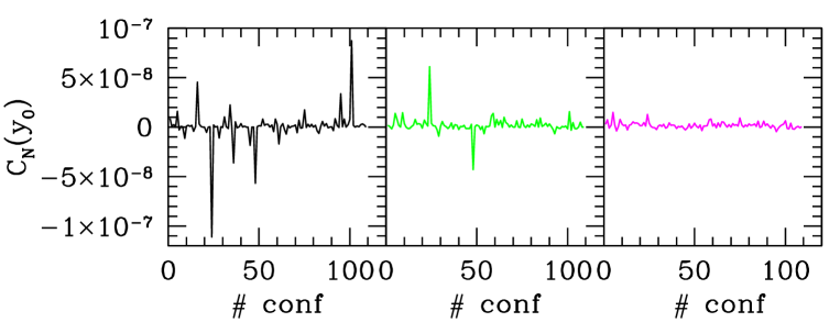
Figure 2: Monte Carlo history of the correlation function $C_{n}(t)$ at $t=y_{0}=9a$, for $am=0.04$.

3 Numerical results and discussion

We tested our method on quenched Neuberger fermions defined on a lattice with $L/a=12$, $T/a=32$, $\beta=5.8485$, corresponding to $a\simeq 0.12$ fm, $L\simeq 1.5$ fm. We used three different quark masses $am=0.04,0.055,0.07$ and collected $N_{\rm{conf}}=109$ measurements of the baryon correlation function. We extracted $n=20$ low modes of the Dirac operator, and chose $n_{b}=20$ for the low-mode averaging on the $hll$ contribution. Taking into account the symmetries of the source vectors $V^{k}$, this corresponds to computing $2n_{b}$ inversions of the propagator. In fig. 1 we show the coefficients $c_{k}$ of eq. (10) for $k=0,...,n_{b}-1$ for a typical configuration at $am=0.04$; they drop off considerably fast, which justifies the restriction $k=0,...,n_{b}-1$ for the application of low-mode averaging. In any case we stress that we performed no systematic study to optimize the choice of the parameter $n_{b}$. In fig. 2 we show the Monte Carlo history of $C_{N}(t)$ at a given time slice $t=y_{0}=9a$, for the lightest mass $am=0.04$. The first figure from the left corresponds to the local computation, and the presence of large fluctuations can be observed.

$am$	$am_{eff}$ (no lma)	$am_{eff}$ (lma on $lll$)	$am_{eff}$ (lma on $lll$+$hll$)
0.04	0.69(62)	0.76(14)	0.78(7)
0.055	0.89(20)	0.81(11)	0.85(6)
0.07	0.94(11)	0.87(8)	0.90(5)

Table 1: Numerical results of low-mode averaging (lma) for the effective mass in units of lattice spacing at $t/a=9$, for different values of the quark mass $am$.

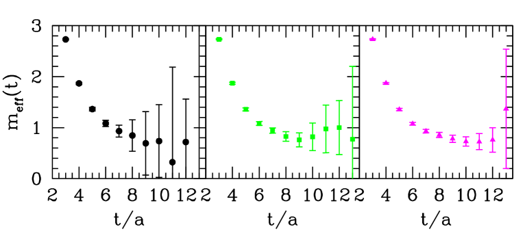
Figure 3: Effective mass for $am=0.04$.

The figure in the centre is obtained by performing low-mode averaging on the $lll$ part of the correlation function, as in eq. (6): the fluctuations are reduced, but nevertheless we still observe residual spikes. Finally, the third curve on the right corresponds to the computation where low-mode averaging is applied to both $lll$ and $hll$ contributions: in this case the large fluctuations are sensibly suppressed. This confirms a posteriori that the fluctuations given by the $lll$ and $hll$ contributions are the dominant ones.
At large time separations, we expect

$$C_{N}(t)=\bigg{[}A_{N}\left(e^{-m_{N}t}-e^{-m_{N}(T-t)}\right)+A_{N^{*}}\left(e^{-m_{N^{*}}t}-e^{-m_{N^{*}}(T-t)}\right)\bigg{]}...,$$ (12)

where $m_{N}$ is the mass of the ground-state positive-parity nucleon, and $m_{N^{*}}$ is the mass of the negative-parity state $N^{*}$ . In table 1 we report the numerical results for the effective mass at $t/a=9$, for our three values of the quark mass. For the local correlator, the fluctuations are such that a jackknife statistical analysis of the errors cannot be trusted, and the uncertainties reported in the first column for $am=0.04$ and $0.055$ are just for completeness. For the lightest-quark mass, low-mode averaging applied on $lll$ and $hll$ with $n_{b}=20$ guarantees a reliable determination of statistical errors. A brute comparison of the errors indicates a reduction by a factor 10, to be compared with an increase of the computational cost by a factor 8. Going to heavier quark masses the low-mode averaging becomes less efficient, as expected; the same effect is foreseen by increasing the volume at fixed quark mass. In fig. 3 we report the results obtained for the nucleon effective mass, for $am=0.04$. On the first figure on the left, no low-mode averaging has been applied, and the signal for the nucleon is very poor. In the centre we show the effect of applying low-mode averaging on the $lll$ part only: for $t/a\gtrsim 7$ we already observe a significant improvement on the signal. Finally, on the right we show the effective mass that we obtain after applying low-mode averaging on $lll$ and $hll$ contributions; here the statistical errors in the range $t/a\sim 9$–$12$ are under control and we can attempt to extract the nucleon mass $m_{N}$. It is important to stress that our uncertainty on the nucleon mass after low-mode averaging is still quite large with respect to the errors obtained without low-mode averaging but with different choices of the nucleon interpolating field (see e.g. [13] for a recent computation). For this reason, as a next step we intend to apply this method to baryon two-point functions with other interpolating fields. Moreover, the technique can be easily generalized to baryon three-point functions and could therefore be very useful for the computation of the electric neutron dipole moment [14, 15].

References

- [1] H. Leutwyler and A. Smilga, Spectrum of Dirac operator and role of winding number in QCD, Phys. Rev. D 46 (1992) 5607.
- [2] E. V. Shuryak and J. J. M. Verbaarschot, Random matrix theory and spectral sum rules for the Dirac operator in QCD, Nucl. Phys. A 560 (1993) 306 [hep-th/9212088].
- [3] P. H. Damgaard, The microscopic Dirac operator spectrum, Nucl. Phys. Proc. Suppl. 106 (2002) 29 [hep-lat/0110192] and references therein.
- [4] P. H. Damgaard, R. G. Edwards, U. M. Heller and R. Narayanan, Universal scaling of the chiral condensate in finite-volume gauge theories, Phys. Rev. D 61 (2000) 094503 [hep-lat/9907016].
- [5] W. Bietenholz, K. Jansen and S. Shcheredin, Spectral properties of the overlap Dirac operator in QCD, JHEP 0307 (2003) 033 [hep-lat/0306022].
- [6] L. Giusti, M. Lüscher, P. Weisz and H. Wittig, Lattice QCD in the epsilon-regime and random matrix theory, JHEP 0311 (2003) 023 [hep-lat/0309189].
- [7] L. Giusti, C. Hoelbling, M. Lüscher and H. Wittig, Numerical techniques for lattice QCD in the epsilon-regime, Comput. Phys. Commun. 153 (2003) 31 [hep-lat/0212012].
- [8] L. Giusti, P. Hernandez, M. Laine, P. Weisz and H. Wittig, Low-energy couplings of QCD from current correlators near the chiral limit, JHEP 0404 (2004) 013 [hep-lat/0402002].
- [9] T. DeGrand and S. Schaefer, Improving meson two-point functions in lattice QCD, Comput. Phys. Commun. 159 (2004) 185 [hep-lat/0401011].
- [10] H. Neuberger, Exactly massless quarks on the lattice, Phys. Lett. B 417 (1998) 141 [hep-lat/9707022]; Vector like gauge theories with almost massless fermions on the lattice, Phys. Rev. D 57 (1998) 5417 [hep-lat/9710089]; More about exactly massless quarks on the lattice, Phys. Lett. B 427 (1998) 353 [hep-lat/9801031].
- [11] P. H. Ginsparg and K. G. Wilson, A remnant of chiral symmetry on the lattice, Phys. Rev. D 25 (1982) 2649.
- [12] M. Lüscher, Exact chiral symmetry on the lattice and the Ginsparg-Wilson relation, Phys. Lett. B 428 (1998) 342 [hep-lat/9802011].
- [13] R. Babich et al., Light hadron and diquark spectroscopy in quenched QCD with overlap quarks on a large lattice, [hep-lat/0509027].
- [14] E. Shintani et al., Neutron electric dipole moment from lattice QCD, Phys. Rev. D 72 (2005) 014504 [hep-lat/0505022].
- [15] T. Blum, these proceedings.