The Gluon Propagator in Lattice Landau Gauge with twisted boundary conditions

Abstract:

We investigate the infrared behaviour of the gluon propagator in Landau gauge on a lattice with twisted boundary conditions.

Analytic calculations using Dyson-Schwinger equations, exact renormalization group and stochastic quantization show that the gluon propagator in Landau gauge approaches zero for small momentum. On the other hand lattice calculations and calculations on a four-torus seem to give rise to a non-zero limit. One possible reason for this difference is the existence of zero-momentum fluctuation modes which potentially give a massive contribution to the gluon propagator. Our simulations show that with twisted boundary conditions these zero-momentum modes are suppressed and the gluon propagator becomes smaller than in a periodic ensemble.

PoS(LAT2005)334

1 Introduction

On $\mathbbm{R}^{4}$ the gluon propagator has been calculated with several techniques, using Dyson-Schwinger equations [1], stochastic quantization [2] and exact renormalization group equation [3]. Representing the gluon propagator in Landau gauge as

$$D_{\mu\nu}^{ab}(p)=\delta^{ab}(\delta_{\mu\nu}-p_{\mu}p_{\nu}/p^{2})D(p^{2})$$ (1)

the low momentum behaviour was found to be $D(p^{2})\stackrel{{\scriptstyle p\to 0}}{{\propto}}(p^{2})^{(2\kappa-1)}$ with $\kappa\approx 0.6$. On the other hand calculations on the torus $\mathbbm{T}^{4}$ using Dyson-Schwinger equations [4] and lattice calculations [5, 6, 7, 8, 9] seem to indicate a non-zero value of $D$ at $p=0$, i.e. $\kappa=0.5$. A possible explanation for the difference between $\mathbbm{R}^{4}$ (non-compact space-time) and $\mathbbm{T}^{4}$ (compact space-time) are zero momentum modes on the compact space-time manifold which potentially give rise to a massive contribution to the gluon propagator.

In this talk we wish to investigate how the implementation of non-trivial boundary conditions changes the infrared behaviour of the gluon propagator.

2 Twisted boundary conditions

To determine the influence of different boundary conditions on the gluon propagator on the lattice (or on the torus) we will consider twisted boundary conditions.

As usual we denote link variables by $U_{\mu}(x)$, the unit vector in $\mu$-direction by $\hat{\mu}$ and the extension of the lattice in $\mu$-direction by $L_{\mu}$. Gauge fixing can be implemented by maximizing some functional $F[g,U]$ with respect to gauge transformations $U_{\mu}(x)\to U^{g}_{\mu}(x)=g^{-1}(x)U_{\mu}(x)g(x+\hat{\mu})$, e.g. for Landau gauge we have $F[g,U]=\sum_{x,\mu}U_{\mu}^{g}(x)$. Non-trivial boundary conditions on the lattice (as well as on the torus) can be introduced by demanding that the link variable is periodic up to a gauge transformation, i.e.

$$U_{\mu}(x+L_{\nu}\hat{\nu})=U_{\mu}^{\Omega_{\nu}}(x)=\Omega_{\nu}^{-1}(x)U_{\mu}(x)\Omega_{\nu}(x+\hat{\mu})\,,$$ (2)

where $\Omega_{\nu}(x)$ is called transition function. This property of the link variable ensures that gauge invariant observables are actually periodic. The transition functions have to fulfill the cocycle condition

$$\Omega_{\nu}(x)\Omega_{\mu}(x+L_{\nu}\hat{\nu})=\Omega_{\mu}(x)\Omega_{\nu}(x+L_{\mu}\hat{\mu})Z_{\mu\nu}\,,$$ (3)

where $Z_{\mu\nu}$ are elements of the center of the gauge group. Twisted boundary conditions imply that some of the group elements $Z_{\mu\nu}$ are non-trivial. Under a general gauge transformation $g$ the transition functions transform as

$$\Omega^{g}_{\mu}(x)=g^{-1}(x)\Omega_{\mu}(x)g(x+L_{\mu}\hat{\mu})$$ (4)

leaving the twists $Z_{\mu\nu}$ unchanged. For twisted boundary conditions gauge fixing is non-trivial: If we implement non-trivial boundary conditions via some transition functions $\Omega_{\mu}(x)$ we should keep these transition functions fixed during gauge fixing, i.e. we have to find the maximum of the gauge fixing functional $F[g,U]$ with respect to such gauge transformations $g$ which do not change the transition functions.

But there is a second problem concerning the choice of transition functions for a given gauge functional $F[g,U]$. Let us consider the Landau gauge in periodic boundary conditions. Maximizing $F[g,U]$ in this case means that we try to make the deviation of the gauge fixed configuration $U^{g}_{\mu}(x)$ from the configuration $U_{\mu}(x)\equiv\mathbbm{1}$ (which corresponds to the absolute maximum of $F$ and which has zero field strength) as small as possible. On the other hand one could (awkwardly) choose non-trivial transition functions and keep them fixed during Landau gauge fixing. Then in general $U_{\mu}(x)\equiv\mathbbm{1}$ will not fulfill these new periodicity properties (2) and some other configuration $\tilde{U}_{\mu}(x)$ will be the maximum of the functional $F[\mathbbm{1},U]$. However, in general this configuration $\tilde{U}_{\mu}(x)$ will have non-zero and non-constant field strength. Landau gauge fixing with these (artificially) introduced transition functions will make the deviation of the gauge fixed configuration $U^{g}_{\mu}(x)$ from $\tilde{U}_{\mu}(x)$ as small as possible. This will obviously destroy translational invariance, which is physically not sensible. The lesson is that one should be careful in choosing the transition functions. If possible one should choose the transition functions (also in the twisted case) such that $U_{\mu}(x)\equiv\mathbbm{1}$ fulfills eq. (2).

From now on we will specialize to the gauge group $SU(2)$. We parametrize the links as usual ($\sigma_{k}$ - Pauli matrices)

$$U_{\mu}(x)=u_{\mu}^{0}(x)\mathbbm{1}+iu_{\mu}^{k}(x)\sigma_{k}\,,\quad u_{\mu}^{j}\in\mathbbm{R}\,,\quad j=0,1,2,3$$ (5)

and choose constant transition functions, so-called twist eaters [10]:

$$\Omega_{0}\equiv\mathbbm{1}\,,\quad\Omega_{k}\equiv i\sigma_{k}\,,\quad k=1,2,3$$ (6)

corresponding to the twists

$$Z_{0k}=\mathbbm{1}\,,\quad k=1,2,3\,,\quad Z_{12}=Z_{23}=Z_{31}=-\mathbbm{1}\,.$$ (7)

From eq. (2) one easily obtains

$$u_{\mu}^{0}(x+L_{k}\hat{k})=u_{\mu}^{0}(x)\,,\quad u^{a}_{\mu}(x+L_{k})=\left\{\begin{array}[]{ll}u^{a}_{\mu}(x)\,,&{\mathrm{if}}\quad k=a\\ -u^{a}_{\mu}(x)\,,&{\mathrm{else}}\end{array}\right.\,,$$ (8)

i.e. some of the colour components are anti-periodic in spatial directions. The vacuum configuration $U_{\mu}(x)\equiv\mathbbm{1}$ fulfills these boundary conditions, which are compatible with Landau gauge.

Now let us have a look at the zero momentum part of the gauge potential. The gauge potential $A_{\mu}(x)$ (corresponding to the links $U_{\mu}(x)$) and and its Fourier transformation are given by

$$A_{\mu}(x) = 1/2(U_{\mu}(x)-U_{\mu}^{+}(x))$$ (9)

$$\tilde{A}_{\mu}(p) = \frac{1}{V}\sum_{x}A_{\mu}(x)e^{ipx}$$ (10)

With periodic boundary conditions the zero-momentum part $C_{\mu}:=\tilde{A}_{\mu}(p=0)$ shows large fluctuations during the simulation [11], as can be seen in fig. 1. These fluctuations and their amplitudes are clearly reduced with twisted boundary conditions.

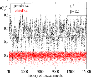
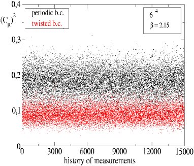
Figure 1: Simulation history of the zero momentum part $C_{\mu}$ in periodic (black) and twisted (red) boundary conditions on a $6^{4}$ lattice with $\beta=10$ (left) and $\beta=2.15$ (right).

At this point let us mention two further advantages of the constant transition functions: They are numerically easy to implement and the periodicity in time allows finite temperature calculations.

The effect of the twisted boundary conditions should become smaller on larger lattices, while for small lattices we expect a strong dependence on the lattice size.

3 The gluon propagator in twisted boundary conditions

We have measured the gluon propagator for different lattice sizes at $\beta=2.15$, see fig. 2.

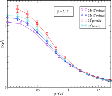
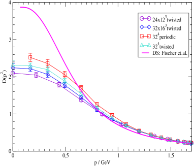
Figure 2: Plot of gluon propagator $D(p^{2})$ with twisted and periodic boundary conditions for different lattice sizes (left) and comparison with results from Dyson-Schwinger equation on the Torus [4].

As can be seen: for larger spatial extension of the lattice the “twisted” gluon propagator becomes larger and the “twisted” gluon propagator is always smaller than the “periodic” gluon propagator, i.e. one can consider the gluon propagator in the twisted ensemble as a lower bound for the gluon propagator in the periodic ensemble. As expected for larger spatial extensions the difference between the propagators with periodic and twisted boundary conditions decreases, i.e. the finite size effects due to the twists become smaller.

All these observations suggest that the gluon propagator $D(p^{2})$ on the lattice has a non-zero limit for $p\to 0$. Furthermore, our results confirm results obtained by solving Dyson-Schwinger equations on the torus [4].

Unfortunately, our investigations do not clarify the difference between compact and non-compact space-times. Our findings seem to indicate that this difference in the infrared behaviour of the gluon propagator remains even in the limit of an infinitely large lattice.

References

- [1] C. Lerche and L. von Smekal, Phys. Rev. D 65, 125006 (2002).
- [2] D. Zwanziger, Phys. Rev. D 65, 094039 (2002).
-
[3]
J. M. Pawlowski, D. F. Litim, S. Nedelko and L. von Smekal,
Phys. Rev. Lett. 93 (2004) 152002
;
C. S. Fischer and H. Gies, JHEP 0410 (2004) 048, -
[4]
C. S. Fischer and R. Alkofer,
Phys. Lett. B 536, 177 (2002);
C. S. Fischer, R. Alkofer and H. Reinhardt, Phys. Rev. D 65, 094008 (2002);
C. S. Fischer, “Infrared exponents of Yang-Mills theory”,these proceedings. - [5] J. Gattnar, K. Langfeld and H. Reinhardt, Phys. Rev. Lett. 93, 061601 (2004).
- [6] A. Sternbeck, E. M. Ilgenfritz, M. Mueller-Preussker and A. Schiller, Phys. Rev. D 72 (2005) 014507.
- [7] F. D. Bonnet et al., Phys. Rev. D 64, 034501 (2001).
- [8] P. O. Bowman, U. M. Heller, D. B. Leinweber, M. B. Parappilly and A. G. Williams, Phys. Rev. D 70 (2004) 034509.
- [9] O. Oliveira and P. J. Silva, AIP Conf. Proc. 756, 290 (2005).
- [10] J. Ambjorn and H. Flyvbjerg, Phys. Lett. B 97, 241 (1980).
- [11] G. Damm,W. Kerler and V.K. Mitrjushkin, Phys. Lett. B 433, 88 (1998).