Structure of the Pion from Full Lattice QCD

Abstract:

Moments of generalised parton distributions can be related to off-forward matrix elements of local operators. We calculate a few of the leading twist matrix elements for the pion on the lattice. The simulations are performed using two flavours of dynamical fermions and a range of pion masses from 550 to 1090 MeV. Our lattice spacings and spatial volumes lie in the range 0.07–0.12 fm and $($1.6–2.2 fm$)^{3}$, respectively. Key features of our investigation are the use of $O(a)$ improved Wilson fermions and non-perturbative renormalisation.

We present first results for the two lowest moments of the generalised parton distributions of the pion and compare the pion electromagnetic form factor $F_{\pi}$ to experimental data. Good agreement is found between lattice data and experiment.

PoS(LAT2005)360

1 Introduction

The pion as a near Goldstone boson is essential for chiral symmetry breaking. It also plays an important role for theoretical models since it is the simplest spinless meson. However, the understanding of the structure of the pion is still limited. On the experimental side results from electroproduction measurements, e.g. $e\,p\to e\,\pi^{+}\,n$, are available and provide information about the pion electromagnetic form factor $F_{\pi}$. Parton distribution functions on the other hand are obtained from Drell-Yan dilepton production processes, $\pi^{\pm}\,N\to\mu^{+}\mu^{-}\,X$, and prompt photon production, i.e. $\pi^{\pm}\,N\to\gamma\,X$. For some time now it has been possible to explore the structure also from first principles using lattice QCD. Initial studies by Martinelli et al. and Draper et al. were performed for the pion form factor and parton distributions [1]. The main interest recently was on the pion form factor [2, 3, 4]. In this contribution we investigate generalised parton distributions (GPDs) of the pion [5, 6, 7].

GPDs can be seen as a generalisation of parton distributions and form factors. They contain both as limiting cases but go beyond that and include new information about the structure of the pion that is not yet accessible by experiments. This work is an extension of earlier studies [8] and complements current efforts on the nucleon structure [9, 10].

2 Generalised Form Factors

GPDs parametrise off-forward matrix elements probing single quarks inside hadrons. Hence the respective structure of hadrons can be described by GPDs. In case of the pion, the vector operator matrix elements on the light-cone with the corresponding GPDs $H^{q}_{\pi}$ read

$$H^{q}_{\pi}(x,\xi,t)=\frac{1}{2\,n\cdot P}\int\frac{\mathrm{d}{\lambda}}{2\pi}\;\mathrm{e}^{\mathrm{i}\lambda n\cdot Px}\left<\pi(p^{\prime})\right|\overline{\psi}_{q}(-\frac{\lambda}{2}n)\;n\cdot\gamma\;\mathcal{U}\,\psi_{q}(\frac{\lambda}{2}n)\left|\pi(p)\right>\,,$$ (1)

where the kinematical variables are the average momentum of the incoming and outgoing pion, $P^{\mu}=\frac{1}{2}(p^{\prime\mu}+p^{\mu})$, the momentum transfer $\Delta^{\mu}=(p^{\prime\mu}-p^{\mu})$ and its invariant form $t=\Delta^{2}$. The fractional longitudinal momentum transfer is $\xi=-(n\cdot\Delta)/(2n\cdot P)$ with a light-like vector $n^{\mu}$. A Wilson line $\mathcal{U}$ is included to ensure gauge invariance. Important properties of $H^{q}_{\pi}(x,\xi,t)$ are:

• In the forward limit, $\Delta\to 0$, one recovers the usual parton distributions. We have $H^{q}_{\pi}(x,0,0)=q(x)$ for $x>0$ and $H^{q}_{\pi}(x,0,0)=-\overline{q}(-x)$ for $x<0$.

• The first moment in $x$ is related to the pion form factor. Starting from a flavour dependent GPD, the full form factor including all quark flavours can be be obtained using isospin relations [6]. Assuming we probe $u$-quarks within a $\pi^{+}$ we find $\int\mathrm{d}x\,H^{u}_{\pi^{+}}(x,\xi,t)=F_{\pi}(t)$.

• Taking the Fourier transform in $\Delta_{\perp}$ results in a probabilistic interpretation in coordinate space. One finds $(2\pi)^{-2}\int\mathrm{d}^{2}\Delta_{\perp}\,\mathrm{e}^{-\mathrm{i}b_{\perp}\cdot\Delta_{\perp}}H^{q}_{\pi}(x,\xi=0,t=-\Delta^{2}_{\perp})=q_{\pi}(x,b_{\perp})$ which is the probability of finding a quark $q$ with momentum fraction $x$ and impact parameter $b_{\perp}$ in the pion [11].

Since Eq. (1) is a light-cone matrix element, it cannot be calculated on the lattice directly. Instead, the operator product expansion is applied to obtain matrix elements of local operators. These matrix elements can then be parametrised by generalised form factors (GFFs), which are proportional to moments of the GPDs [5, 6]. The GFFs thus provide an equivalent description of the hadron structure. The operators $\mathcal{O}^{\{\mu\mu_{1}\mu_{2}\dots\mu_{n}\}}$ and the decomposition of their matrix elements into GFFs corresponding to Eq. (1) read (assuming from now on that we probe $u$-quarks within a $\pi^{+}$)

$$\left<\pi^{+}(p^{\prime})\right|\mathcal{O}^{\{\mu\mu_{1}\mu_{2}\dots\mu_{n}\}}\left|\pi^{+}(p)\right>=\left<\pi^{+}(p^{\prime})\right|\overline{u}(0)\,\gamma^{\{\mu}\,\mathrm{i}\raisebox{0.89996pt}{$\stackrel{{\scriptstyle\scriptstyle\leftharpoonup\rightharpoonup}}{{D}}$}\/^{\mu_{1}}\mathrm{i}\raisebox{0.89996pt}{$\stackrel{{\scriptstyle\scriptstyle\leftharpoonup\rightharpoonup}}{{D}}$}\/^{\mu_{2}}\dots\mathrm{i}\raisebox{0.89996pt}{$\stackrel{{\scriptstyle\scriptstyle\leftharpoonup\rightharpoonup}}{{D}}$}\/^{\mu_{n}\}}\,u(0)\left|\pi^{+}(p)\right>=\\ 2\;P^{\{\mu}P^{\mu_{1}}\dots P^{\mu_{n}\}}A_{n+1,0}(\Delta^{2})+\;2\sum^{n}_{\begin{subarray}{c}i=1\\ \textrm{odd}\end{subarray}}\Delta^{\{\mu}\Delta^{\mu_{1}}\dots\Delta^{\mu_{i}}P^{\mu_{i+1}}\dots P^{\mu_{n}\}}\,A_{n+1,i+1}(\Delta^{2})\,,$$ (2)

where $n$ labels the number of covariant derivatives $\raisebox{0.89996pt}{$\stackrel{{\scriptstyle\scriptstyle\leftharpoonup\rightharpoonup}}{{D}}$}=\frac{1}{2}(\raisebox{0.89996pt}{$\stackrel{{\scriptstyle\scriptstyle\rightharpoonup}}{{D}}$}-\raisebox{0.89996pt}{$\stackrel{{\scriptstyle\scriptstyle\leftharpoonup}}{{D}}$})$ and $\{\dots\}$ indicates symmetrisation of indices and subtraction of traces. The GFFs are denoted by $A_{n,i}$. This decomposition is constrained by Lorentz invariance, parity, and time reversal, the latter requiring an even number of momenta $\Delta$. The simplest case $n=0$ of Eq. (2) yields the pion electromagnetic form factor $\left<\pi(p^{\prime})\right|\mathcal{O}^{\mu}\left|\pi(p)\right>=2\,P^{\mu}F_{\pi}(\Delta^{2})$, thus we have $A_{1,0}=F_{\pi}$.

3 Lattice Techniques

The calculation of the matrix elements and the extraction of GFFs in (2) is done in analogy to the nucleon case. We compute pion two- and three-point functions in order to isolate the observables in question [9, 10]. Inserting complete sets of energy eigenstates and employing translational invariance, the three-point function takes the following form for $t<t_{\text{sink}}$

$$C_{\pi\mathcal{O}\pi}(t,p^{\prime},p)=\left<\pi(p^{\prime})\right|\mathcal{O}(t)\left|\pi(p)\right>\frac{\left<0\right|\eta_{\pi}(\vec{p}^{\prime})\left|\pi(p^{\prime})\right>\left<\pi(p)\right|\eta_{\pi}^{\dagger}(\vec{p})\left|0\right>}{2E_{p^{\prime}}\,2E_{p}}\text{e}^{-E_{p^{\prime}}(t_{\text{sink}}-t)-E_{p}\,t}+\dots\,,$$ (3)

where we omit excited states and set $t_{\text{source}}=0$. Here $\eta_{\pi}(\vec{p})$ is the interpolating field for a pion with momentum $\vec{p}$ and energy $E_{p}$ the corresponding energy. We use both pseudo-scalar and axial vector interpolators. The two-point function, again omitting higher energy states, has the usual form

$$C_{\pi\pi}(t,p)=\frac{\left<0\right|\eta_{\pi}(\vec{p})\left|p\right>\left<p\right|\eta_{\pi}^{\dagger}(\vec{p})\left|0\right>}{2E_{p}}\text{e}^{-E_{p}T/2}\cosh[E_{p}(T/2-t)]+\dots\,,$$ (4)

with the time extent $T$ of the lattice. We then construct an appropriate ratio of two- and three-point functions to eliminate the exponential time behaviour and the overlap factors such as $\left<0\right|\eta_{\pi}(\vec{p}^{\prime})\left|\pi(p^{\prime})\right>$ that appear in Eq. (3). In doing so we avoid having to fit the energies $E_{p}$ and the normalisation separately. We choose $t_{\text{sink}}=T/2$ so that the three-point correlator is symmetric under $t\to T-t$. The ratio that can then be used is

$$\frac{\left<p^{\prime}\right|\mathcal{O}(t)\left|p\right>}{4\sqrt{E_{p^{\prime}}E_{p}}}=\frac{C_{\pi\mathcal{O}\pi}(t,p^{\prime},p)}{C_{\pi\pi}(t_{\text{sink}},p^{\prime})}\;\left(\frac{C_{\pi\pi}(t_{\text{sink}}-t,p)\,C_{\pi\pi}(t,p^{\prime})\,C_{\pi\pi}(t_{\text{sink}},p^{\prime})}{C_{\pi\pi}(t_{\text{sink}}-t,p^{\prime})\,C_{\pi\pi}(t,p)\,C_{\pi\pi}(t_{\text{sink}},p)}\right)^{\frac{1}{2}}\,.$$ (5)

The l.h.s. now contains the matrix element we are interested in. Hence we can extract the GFFs from matching the lattice ratio (5) to its continuum parametrisation Eq. (2). Using all momentum combinations and operators available, this results in an over-constrained fit of the $A_{n,i}(\Delta^{2})$.

Contributions from excited states with energy $E^{\prime}$ to the ratio (5) are suppressed as long as $t_{\text{sink}}-t\gg 1/E^{\prime}$ and $t\gg 1/E^{\prime}$. However, because of the exponential decay of the pion two-point function, the signal at $t=t_{\text{sink}}$ for non-vanishing momenta is poor and can take negative values. This causes problems when taking the square root. We can partly circumvent this by shifting the two-point function, i.e. changing $C_{\pi\pi}(t_{\text{sink}},p)\to C_{\pi\pi}(t_{\text{sink}}-t_{\text{shift}},p)$. This shift is compensated by an extra factor of $(\cosh(E_{p}\,t_{\text{shift}}))^{-1}$ to the two-point function.

The operators we use are all constructed to be traceless and symmetric. Along with more details like transformation and mixing properties, they are given in [12].

4 Results

Our simulation is performed with two flavours of non-perturbatively clover-improved dynamical Wilson fermions and Wilson glue. We use operators with up to three derivatives [12] and exploit the full Clifford-Algebra, i.e. we calculate (pseudo-) scalar, (pseudo-) vector, and tensor currents. The combinations involving $\gamma_{5}$ should vanish due to the symmetry properties of (2) under parity and we use this as a check for our calculations. The large number of momentum combinations for the over-constrained fit to the GFFs is achieved by using three sink momenta $\vec{p}^{\prime}$ and 17 momentum transfers $\vec{\Delta}=\vec{p}^{\prime}-\vec{p}$, which in lattice units $\times L/2\pi$ are given by:

• $(0,0,0)$, $(0,-1,0)$, $(-1,0,0)$,

• $(0,0,0)$, $(1,0,0)$, $(1,1,0)$, $(1,1,1)$, $(2,0,0)$, $(2,1,1)$, and permutations w.r.t. the components.

A list of further parameters of our simulation can be found in Table 1. The configurations have been generated within the QCDSF and UKQCD collaborations.

$\beta$	5.20	5.20	5.20	5.25	5.25	5.25	5.29	5.29	5.29	5.40	5.40	5.40
$\kappa$	.13420	.13500	.13550	.13460	.13520	.13575	.13400	.13500	.13550	.13500	.13560	.13610
$m_{\pi}$ [GeV]	.94	.777	.578	.92	.774	.553	1.09	.867	.716	.969	.788	.588
$L$ [fm]	1.96	1.68	1.59	1.69	1.56	2.19	1.66	1.53	2.16	1.97	1.88	1.79
$m_{\pi}\cdot L$	9.36	6.64	4.66	7.89	6.11	6.14	9.23	6.74	7.85	9.68	7.48	5.3

Table 1: Our set of lattices available. Highlighted columns mark the current data points.

The connection to physical values is done using the Sommer scale with $r_{0}=0.5$ fm and non-perturbative renormalisation [13]. The results have finally been converted to the $\overline{\text{MS}}$-scheme at $\mu=2{\,\text{Ge}\kern-0.66666pt\text{V\/}}$.

Comparing both interpolating fields for the pion, we find a cleaner signal for the axial vector current. Using this interpolator we extract values for $A_{1,0}$ and $A_{2,0}$. Results for $A_{1,0}$, the pion electromagnetic form factor, can be found in Fig. 3. We use a monopole ansatz $(1-t/m_{\textrm{mono}}^{2})^{-1}$ to fit our data and find that the monopole mass decreases with decreasing pion masses as expected. A linear chiral extrapolation of the monopole masses, shown in Fig. 3, provides a mass of $736(36){\,\text{Me}\kern-0.66666pt\text{V\/}}$ in the chiral limit. This is in nice agreement with experimental data, as shown by the bottom curve in Fig. 3. Scaling violations are expected to be small and will be investigated in more detail at a later stage when the analysis is completed for all lattices.

In Fig. 3 we show $A_{1,0}$ and $A_{2,0}$ for one of our data sets, both normalised to 1 at $t=0$ for better comparison. The flattening of the slope for higher moments corresponds to a narrower spatial distribution of partons within impact parameter space for $x\to 1$ [11].

From the value of $A_{2,0}$ at $t=0$ we can determine the quark content and the corresponding momentum fraction in the pion. For the data set shown in Fig. 3 the renormalised value for the second moment is $2\,A_{2,0}(t=0)=0.631(16)$, meaning that the quarks and antiquarks within the pion carry about two thirds of the pion’s momentum.

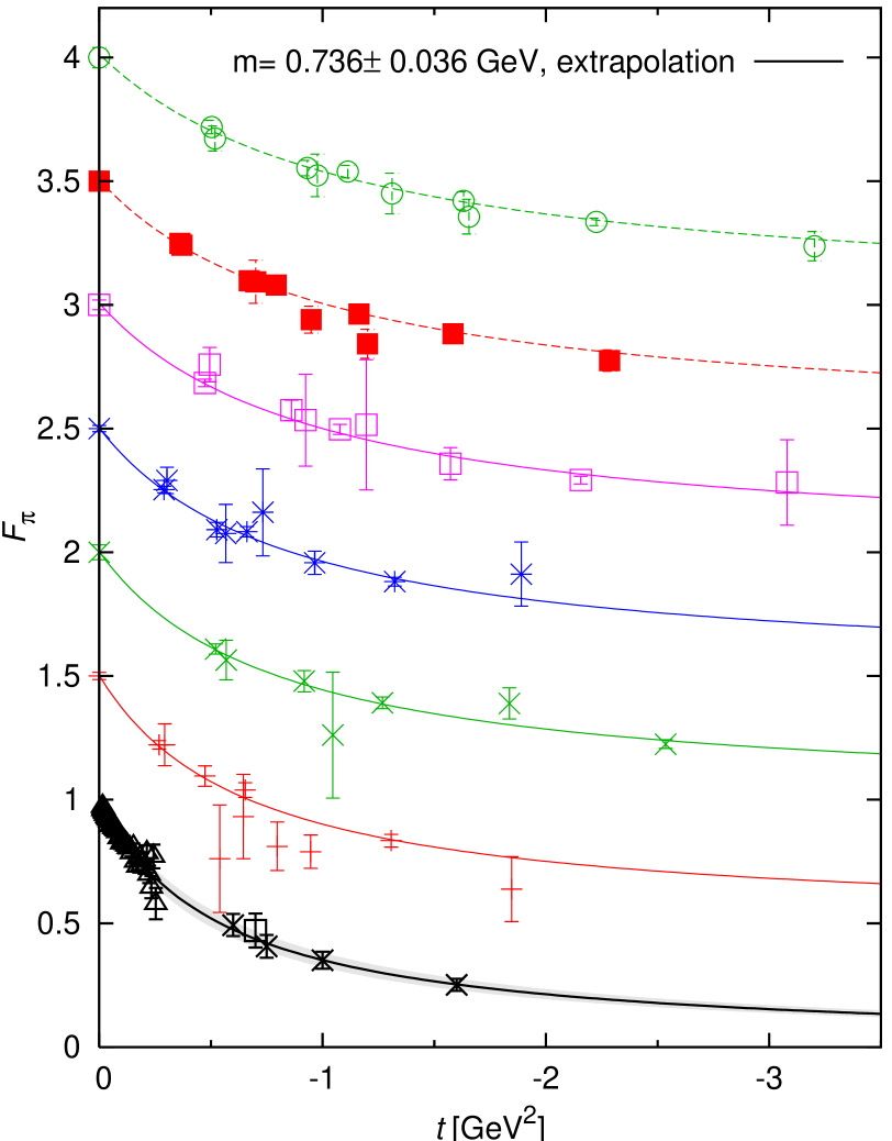
Figure 1: Pion form factor $F_{\pi}(t)$ for our different lattices (with different offsets). The pion masses decrease from top to bottom with fitted monopole masses: $1066(43){\,\text{Me}\kern-0.66666pt\text{V\/}}$, $1005(18){\,\text{Me}\kern-0.66666pt\text{V\/}}$, $993(28){\,\text{Me}\kern-0.66666pt\text{V\/}}$, $926(24){\,\text{Me}\kern-0.66666pt\text{V\/}}$, $892(32){\,\text{Me}\kern-0.66666pt\text{V\/}}$, and $817(26){\,\text{Me}\kern-0.66666pt\text{V\/}}$. Also included is the extrapolation to the physical pion mass with a comparison to experimental data (black curve and symbols).

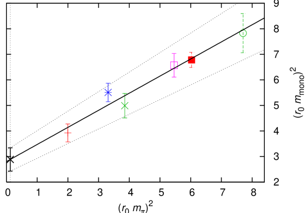
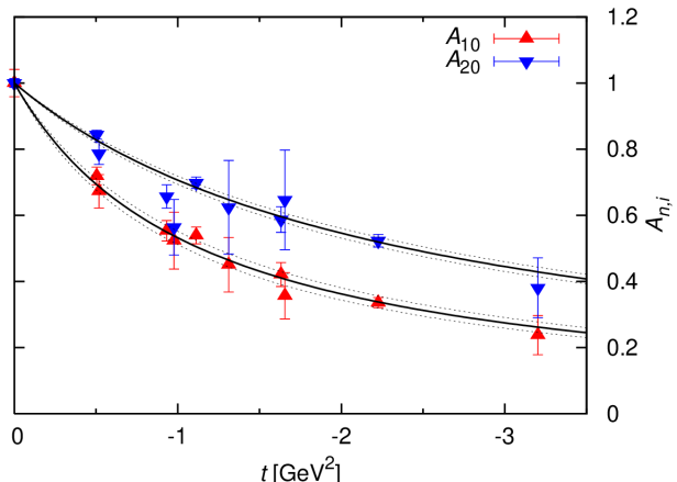
Figure 2: Linear chiral extrapolation of the monopole masses to the physical $m_{\pi}$.

Figure 3: First and second moment, $A_{1,0}$ and $A_{2,0}$, of the pion GPD [$\beta=5.29$, $\kappa=0.13400$].

5 Outlook

The above analysis will be completed for all our lattices, and we have more data for higher moments with up to three derivatives. The calculations include not only the vector operators, but also the tensor combinations mentioned above. We will furthermore be able to increase our statistics by using the symmetry properties w.r.t. $t_{\text{sink}}$ of our three-point correlation function.

References

- [1] G. Martinelli and C. T. Sachrajda, A lattice calculation of the pion’s form-factor and structure function, Nucl. Phys. B306 (1988) 865; T. Draper, R. M. Woloshyn, W. Wilcox, and K.-F. Liu, The pion form-factor in lattice QCD, Nucl. Phys. B318 (1989) 319.
- [2] F. D. R. Bonnet, R. G. Edwards, G. T. Fleming, R. Lewis, and D. G. Richards, Lattice computations of the pion form factor, Phys. Rev. D72 (2005) 054506, [hep-lat/0411028].
- [3] J. van der Heide, J. H. Koch, and E. Laermann, Pion structure from improved lattice QCD: Form factor and charge radius at low masses, Phys. Rev. D69 (2004) 094511, [hep-lat/0312023].
- [4] S. Capitani, C. Gattringer, and C.B. Lang, Pion form factor with chirally improved fermions, PoS(LAT2005)126 (2005) [hep-lat/0509023].
- [5] A. V. Belitsky and A. V. Radyushkin, Unraveling hadron structure with generalized parton distributions, hep-ph/0504030.
- [6] M. Diehl, Generalized parton distributions, Phys. Rept. 388 (2003) 41, [hep-ph/0307382].
- [7] K. Goeke, M. V. Polyakov, and M. Vanderhaeghen, Hard exclusive reactions and the structure of hadrons, Prog. Part. Nucl. Phys. 47 (2001) 401, [hep-ph/0106012].
- [8] C. Best et al., Pion and rho structure functions from lattice QCD, Phys. Rev. D56 (1997) 2743, [hep-lat/9703014].
- [9] QCDSF Collaboration, M. Göckeler et al., Quark helicity flip generalized parton distributions from two-flavor lattice QCD, hep-lat/0507001; QCDSF Collaboration, M. Göckeler et al., Generalized parton distributions and transversity from full lattice QCD, hep-lat/0501029.
- [10] LHPC and SESAM Collaborations, Ph. Hägler et al., Transverse structure of nucleon parton distributions from lattice QCD, Phys. Rev. Lett. 93 (2004) 112001, [hep-lat/0312014]; LHPC and SESAM Collaborations, Ph. Hägler et al., Moments of nucleon generalized parton distributions in lattice QCD, Phys. Rev. D68 (2003) 034505, [hep-lat/0304018].
- [11] M. Burkardt, Impact parameter space interpretation for generalized parton distributions, Int. J. Mod. Phys. A18 (2003) 173, [hep-ph/0207047].
- [12] M. Göckeler et al., Lattice operators for moments of the structure functions and their transformation under the hypercubic group, Phys. Rev. D54 (1996) 5705, [hep-lat/9602029].
- [13] G. Martinelli, C. Pittori, C. T. Sachrajda, M. Testa, and A. Vladikas, A general method for nonperturbative renormalization of lattice operators, Nucl. Phys. B445 (1995) 81, [hep-lat/9411010]; M. Göckeler et al., Nonperturbative renormalisation of composite operators in lattice QCD, Nucl. Phys. B544 (1999) 699, [hep-lat/9807044]; QCDSF Collaboration, M. Göckeler et al., A lattice determination of moments of unpolarised nucleon structure functions using improved Wilson fermions, Phys. Rev. D71 (2005) 114511, [hep-ph/0410187].
- [14] UKQCD Collaboration, C. R. Allton et al., Effects of non-perturbatively improved dynamical fermions in qcd at fixed lattice spacing, Phys. Rev. D65 (2002) 054502, [hep-lat/0107021].