B meson decays at high velocity from mNRQCD

Abstract:

The moving NRQCD (mNRQCD) formalism facilitates the simulation of heavy meson decays at large recoil. We present preliminary results for a number of quantities including the energy splittings and the $B$ meson decay constant that demonstrate that the formalism is accurate over a range of momenta.

PoS(LAT2005)219

1 Introduction

At present there is much work being done to establish accurate values for certain CKM matrix elements and this requires the comparison of theory and experiment for exclusive semileptonic decays of heavy mesons. For example, a value for the CKM matrix element $V_{ub}$ can be obtained from the exclusive semileptonic heavy decay $B\rightarrow\pi l\nu$ but only when it is combined with the corresponding QCD form factor. Theoretically, the calculation of such form factors necessitates a non-perturbative handling of QCD, to which the lattice is ideally suited. Indeed, current lattice simulations work well within the low recoil region (high $q^{2}$). However, gaining access to the full kinematic regime is problematic due to the fact that the final state meson can have large recoil momentum in the rest frame of the initial heavy meson, resulting in large discretisation errors and noisier signals that increase the statistical error. Thus comparisons between theory and experiment have been restricted to the low recoil region. Accessing the form factors at high recoil is particularly important since much of the experimental data lies within this kinematic region.

The ultimate goal of this work is therefore to extend the form factor calculations to cover the entire kinematic range. These techniques can be applied to different semileptonic decays, but here we focus on the most extreme case, $B\rightarrow\pi l\nu$. Lattice calculations are usually carried out in the rest frame of the $B$ meson, however, the approach in mNRQCD is to treat the $B$ meson in a moving frame, whilst maintaining control over the systematic errors. This is achieved by finding the optimal reference frame in which the discretisation and statistical errors are minimised, and then using a mNRQCD action to prevent large discretisation errors associated with the $B$ meson. The central argument for this approach is that although the heavy quark carries almost all the heavy meson momentum, the internal dynamics of the meson are essentially non-relativistic. Previous work in this field includes [1, 2, 3].

1.1 Reference frame

For the most extreme kinematic case, $q^{2}(=p_{B}^{2}-p_{\pi}^{2})=0$, we need to find a frame that minimises both the statistical errors that depend on the average kinetic energy, and the discretisation errors that depend on the momenta. In the case of the statistical errors, the frame in which the kinetic energy is at a minimum is ${\bf p_{B}}={\bf p_{\pi}}$. However, it is possible to have ${\bf p_{\pi}}$ lower as larger values for ${\bf p_{B}}$ can be dealt with using more elaborate sources to reduce the statistical error. The discretisation errors are analysed by considering the momentum flow within the $B$ and $\pi$ mesons and the optimal frame lies within these bounds.

By choosing a reference frame in which the $B$ meson is moving, this reduces the error associated with the pion’s momentum, but increases the error from the $B$ meson’s momentum. However, most of the $B$ meson momentum is carried by the $b$ quark and so we can construct a moving NRQCD Lagrangian to deal with this. To minimise errors associated with the light quark action and light meson momentum, it is essential that the light quark action is $O(a^{2})$ improved.

1.2 mNRQCD

In constructing the mNRQCD Lagrangian, the total momentum of the $b$ quark is defined as $P_{b}^{\mu}={m_{b}u^{\mu}}+{k^{\mu}}$, where the first term is the average momentum and $u^{\mu}=P_{B}/m_{b}=\gamma(1,{\bf v})$ is the 4-velocity. The second term, $k^{\mu}$ is the residual momentum, which is of the same order as the light quark’s momentum. The strategy is to treat the $b$ quark’s average momentum exactly, whilst discretising the residual momentum. The mNRQCD Lagrangian can be derived in two ways. One can either start with the NRQCD Lagrangian (derived from the FWT transformation on the usual relativistic quark fields) and boost the fields, or, one can re-write the Lagrangian in terms of boosted fields and then perform the FWT transformation, we outline the latter. Further details are given in Ref. [4].

In the NRQCD formalism, the FWT transformation is applied to the quark fields in order to decouple the quark from the anti-quark, greatly simplifying the numerics. It also removes the rest energy from the Lagrangian, thus leading to smaller discretisation errors. The decoupling is performed as an expansion in the heavy quark mass or the internal quark velocity and is optimal for small 3-momentum. However, the heavy quark in $B$ decays has very large 3-momentum that is boosted with respect to the lattice frame ($P_{b}$) and therefore it is not possible to apply a FWT transformation on the fields. However, by re-writing the Lagrangian in terms of boosted fields and operators, a FWT transformation can then be applied

$\Psi=\frac{\Lambda({\bf v})}{\sqrt{\gamma}}Te^{-imu.x}A_{D_{t}}\left(\begin{array}[]{c}\psi_{v}\\ \chi_{v}\end{array}\right)$;          $\Lambda=\frac{1}{\sqrt{2(1+\gamma)}}\left(\begin{array}[]{cc}1+\gamma&\sigma.{\bf v}\\ \sigma.{\bf v}&1+\gamma\end{array}\right)$

to give the mNRQCD Lagrangian

$$L=\psi^{\dagger}\left(iD_{t}+i{\bf v.D}+\frac{{\bf D}^{2}}{2\gamma m}-\frac{({\bf v.D})^{2}}{2\gamma m}+\frac{{\bf\sigma.\tilde{B}}}{2\gamma m}\ldots\right)\psi.$$

In addition to the usual terms appearing in the NRQCD Lagrangian, there are now terms that are a function of the 3-velocity of the $b$ quark, ${\bf v}$.

2 Details of current work

Here we define the time evolution operators that are currently being tested and outline the details of the lattice calculation.

2.1 mNRQCD action

From the mNRQCD Lagrangian, the time evolution operator is given by

$${\bf H}=\left(1-\frac{{aH_{0}}}{2n}\right)^{n}_{t}\left(1-\frac{{\delta H}}{2}\right)_{t}U_{4,t-1}^{\dagger}\left(1-\frac{{\delta H}}{2}\right)_{t-1}\left(1-\frac{{H_{0}}}{2n}\right)^{n}_{t-1}$$

Early tests have been carried out for the simplest action, where

$${H_{0}} = -\frac{\Delta^{(2)}}{2m_{Q}}-{\bf v.}\Delta^{(\pm)}+({\bf v.}\Delta^{(\pm)})^{2}\left(\frac{c_{v}}{2m\gamma}+\frac{c_{ct}}{2n}\right),$$

and tests are now being carried out on the fully $O(1/m)$ improved case, where

$${\delta H} = \frac{{\bf\sigma.\tilde{B}}}{2m\gamma}-\frac{c_{c,1}}{m\gamma}\{{\bf v.}\Delta^{(\pm)},\Delta^{(2)}\}-\frac{c_{c,2}}{m\gamma}\left({\bf v.}\Delta^{(\pm)}\right)^{3}+\frac{c_{c,6}}{6}v_{i}\Delta_{i}^{+}\Delta_{i}^{\pm}\Delta_{i}^{-}$$

$$\,\,\frac{c_{c,7}}{m\gamma}\Delta^{(\pm)^{(4)}}+\left(\frac{c_{c,8}}{m\gamma}+\frac{c_{c,9}}{n_{1}}\right)\{{\bf v.}\Delta^{(\pm)},v_{i}\Delta_{i}^{+}\Delta_{i}^{\pm}\Delta_{i}^{-}\}.$$

Note that all the coefficients (labelled $c$) are 1 at tree-level.

2.2 Simulation details

This work was carried out on a $12^{3}\times 24$ lattice with inverse lattice spacing $a^{-1}=1.36(14)$GeV (set from Upsilon splitting) for a data set of 243 quenched configurations. The light quark propagators were generated using clover fermions ($\kappa\sim\kappa_{s}$). Gaussian smearing was used at the source and both local and Gaussian smearing was used at the sink. The heavy quark propagators were generated using both the simplest and $O(1/m)$ improved action. Local and APE smearing was used at both source and sink. The heavy quark mass ($am_{Q}$) ranges from 2-8, where 4 corresponds to the mass of the $b$ quark on this lattice and we looked at a range of velocities, ${\bf v}/c=0-0.8$.

3 Perturbation theory

As with NRQCD, mNRQCD is constructed from a set of non-renormalisable interactions, each of which is accompanied by a coefficient which must be calculated perturbatively in order to obtain physical results. The one-loop parameters which make up the self energy include the energy shift, mass and wavefunction renormalisation and also, the velocity renormalisation which results from the division of the total heavy quark momentum into average and residual pieces. A remnant of reparameterisation invariance on the lattice prevents this coefficient from becoming too large. The inverse quark propagator can be written as a combination of the free propagator and the heavy quark’s self energy,

$$G^{-1} = Q^{-1}-a\Sigma(k)$$

$$= -ik_{4}-\alpha_{s}\Omega_{0}+\alpha_{s}ik_{4}\Omega_{1}+{\bf v.k}-\alpha_{s}{\bf v.k}\Omega_{v}+\ldots$$

$$= {Z_{\psi}}\left(-i\bar{k_{4}}+\frac{{\bf k}^{2}}{2\gamma_{R}m_{R}}+\frac{{\bf P_{R}.k}}{\gamma_{R}m_{R}}+\ldots\right)$$

where the renormalisation constants, eg. ${Z_{\psi}}$, are expressed in terms of the coefficients, $\Omega_{n}$, appearing in the self energy. The value of each $\Omega_{n}$ is obtained by differentiation, further details of which are given in Ref. [5].

4 Testing mNRQCD

There are a variety of quantities that can be computed (for both heavy-heavy (HH) and heavy-light (HL) mesons) at different values of the bare velocity in order to check that mNRQCD is working correctly and that the renormalisations, such as $Z_{P}$, are under control. Such quantities include the kinetic mass, the binding energy, decay constants and energy splittings. The kinetic mass, $M_{\mathrm{kin}}$ is extracted from the dispersion relation

$$E_{v}(k)+C=\sqrt{(Z_{P}{\bf P}_{0}+{\bf k})^{2}+M_{kin}^{2}}$$

where ${\bf P}_{0}=\gamma m{\bf v}$. Figure 2 shows that the kinetic mass (for the HH meson) is fairly constant as a function of the bare velocity, an important feature as it means that the bare quark mass will not have to be retuned to give the correct quark mass as the velocity increases. In figure 2, we plot the ground state energy, $E_{\mathrm{sim}}$ and the binding energy ($=E_{\mathrm{sim}}-E_{0}$), where $E_{0}$ is calculated from perturbation theory. The velocity dependence has largly been removed in the subtracted case. In figure 4, we compare the non-perturbative and perturbative values for the momentum renormalisation $Z_{P}$. The non-perturbative result uses the dispersion relation to compute $Z_{P}$ from $E_{\bf v}({\bf k})$. Figure 4 is a plot of the $\eta_{B}$ decay constant from the $A_{0}$ channel from both NRQCD and mNRQCD. The plot is a ratio of the decay constant at varying total momentum ($P_{\mathrm{tot}}$) over zero $P_{\mathrm{tot}}$. In the NRQCD case, the discretisation errors become dominant at very low $P_{\mathrm{tot}}$, whereas the mNRQCD ratio is constant. Figure 6 shows the same ratio but the numerator comes from the $A_{k}$ channel. This is slightly larger than one, but should come down to one as relativistic corrections are included. Finally, in figure 6 we present a preliminary plot for the hyperfine splitting in the HH case from the NRQCD and $O(1/m)$ improved mNRQCD action.

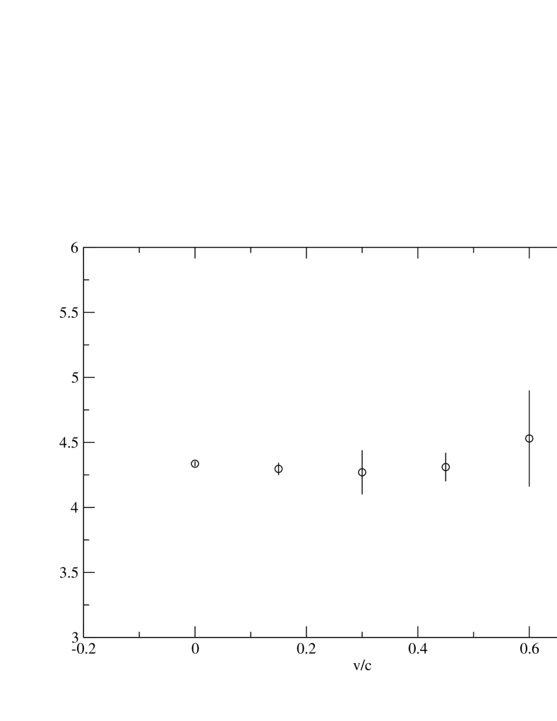
Figure 1: The HH kinetic mass as a function of the velocity from the simplest mNRQCD action.

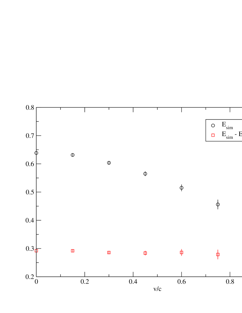
Figure 2: The HL ground state and binding energy at zero residual momentum. Note that binding energy is constant with increasing velocity.

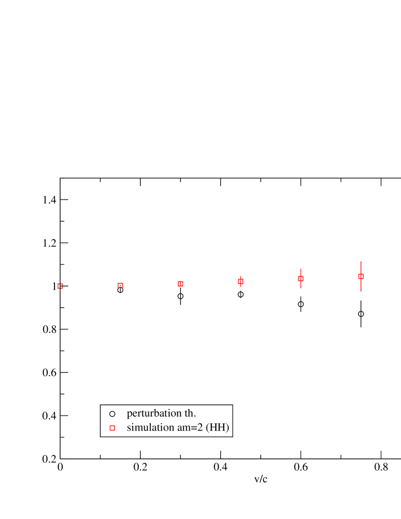
Figure 3: Comparison between the simulated and perturbative velocity renormalisation in mNRQCD.

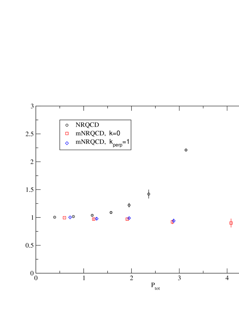
Figure 4: Comparison between the $\eta_{B}$ decay constant from the $A_{0}$ channel in NRQCD and mNRQCD. The mNRQCD data is plotted for two different values of the the residual momentum.

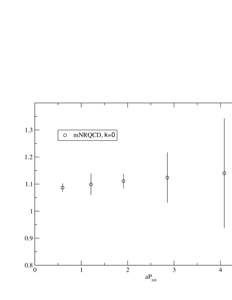
Figure 5: The ratio of the $\eta_{B}$ decay constant from the $A_{k}$ channel and the $A_{0}$ channel. Note there is no leading order term in the NRQCD case, so the leading order answer is zero.

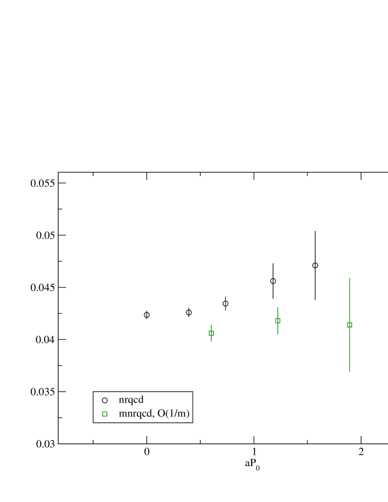
Figure 6: Comparison of the HH hyperfine splitting in NRQCD and $O(1/m)$ improved mNRQCD.

5 Summary

We have presented a number of quantities computed from mNRQCD that demonstrate its applicability to high recoil processes in which the heavy quark carries large external momentum. Future work will focus on computing the $B\rightarrow\pi$ form factor. Due to the complicated nature of a 2-loop perturbative calculation, the intention is to employ numerical techniques to obtain the associated renormalisation coefficients.

References

- [1] S. Hashimoto and H. Matsufuru, Lattice heavy quark effective theory and the isgur-wise function, Phys. Rev. D54 (1996) 4578–4584, [hep-lat/9511027].
- [2] J. E. Mandula and M. C. Ogilvie, Nonperturbative evaluation of the physical classical velocity in the lattice heavy quark effective theory, Phys. Rev. D57 (1998) 1397–1410, [hep-lat/9703020].
- [3] J. H. Sloan, Moving nrqcd, Nucl. Phys. Proc. Suppl. 63 (1998) 365–367, [hep-lat/9710061].
- [4] K. M. Foley, Phd thesis, Cornell University, 2004.
- [5] HPQCD Collaboration, A. Dougall, C. T. H. Davies, K. M. Foley, and G. P. Lepage, The heavy quark’s self energy from moving nrqcd on the lattice, Nucl. Phys. Proc. Suppl. 140 (2005) 431–433, [hep-lat/0409088].