Non-perturbative plaquette in 3d pure SU(3)

Abstract:

We present a determination of the elementary plaquette and, after the subsequent ultraviolet subtractions, of the finite part of the gluon condensate, in lattice regularization in three-dimensional pure SU(3) gauge theory. Through a change of regularization scheme to $\overline{\mbox{\rm MS}}$ and a matching back to full four-dimensional QCD, this result determines the first non-perturbative contribution in the weak-coupling expansion of hot QCD pressure.

PoS(LAT2005)174

1 Introduction

The asymptotic freedom of QCD guarantees a small coupling constant $g$ at large temperatures $T$. While observables can be expressed in a generalized power series in $g$, the loop expansion is not applicable to an arbitrary order in $g$, because of the so-called “infrared wall”, as pointed out by Linde [1] (see also ref. [2]). For every observable there exists an order of the perturbative expansion to which an infinite number of Feynman diagrams contributes. For the pressure this order is $g^{6}T^{4}$.

No way of resumming these infinitely many diagrams has been found, so a different approach is needed. The problem arises due to infrared divergences in the dynamics of zero Matsubara frequency modes of gauge fields. Because these modes are three-dimensional (3d) we can construct an effective 3d pure gauge theory called Magnetostatic QCD (MQCD) which accounts for the non-perturbative contribution [3, 4, 5]. QCD and MQCD can be matched to each other by using perturbation theory.

To obtain the non-perturbative contribution we perform lattice measurements in MQCD [6]. The observable we consider is the elementary plaquette expectation value. The theory being super-renormalisable, one can match the lattice regularization scheme exactly to the $\overline{\textrm{MS}}$ scheme. This requires a perturbative 4-loop computation on the lattice, however, which has not been completed yet: the missing ingredient is specified below. (A certain perturbative 4-loop computation in full QCD remains also to be carried out.)

2 Relation between $\overline{\textrm{MS}}$ and lattice regularization schemes

The euclidean pure SU($N_{\rm c}$) Yang-Mills action reads

$$S_{\textrm{E}}=\int\!\textrm{d}^{d}x\,\mathcal{L}_{\textrm{E}},\quad\quad\mathcal{L}_{\textrm{E}}=\frac{1}{2g_{3}^{2}}\sum_{k,l}\textrm{Tr}[F^{2}_{kl}],$$ (1)

where $d=3-2\epsilon$, $g_{3}^{2}$ is the gauge coupling, $k,l=1,\dots,d$, $F_{kl}=i[D_{k},D_{l}]$, $D_{k}=\partial_{k}-iA_{k}$, $A_{k}=A_{k}^{a}T^{a}$, and $T^{a}$ are hermitean generators of SU($N_{\rm c}$) normalised such that $\textrm{Tr}[T^{a}T^{b}]=\delta^{ab}/2$. The vacuum energy density is defined as

$$f_{\overline{\textrm{MS}}}\equiv-\lim_{V\rightarrow\infty}\frac{1}{V}\ln\left[\int\!\mathcal{D}A_{k}\,\exp\left(-S_{\textrm{E}}\right)\right]_{\overline{\textrm{MS}}},$$ (2)

where $V$ denotes the $d$-dimensional volume. The use of the $\overline{\textrm{MS}}$ dimensional regularization scheme removes any $1/\epsilon$ poles from the expression. In fact, using dimensional regularization the perturbative result vanishes, because there are no mass scales in the propagators. However, for dimensional reasons, the non-perturbative form of the answer is

$$f_{\overline{\textrm{MS}}}=-g_{3}^{6}\frac{d_{A}N_{\rm c}^{3}}{(4\pi)^{4}}\left[\left(\frac{43}{12}-\frac{157}{768}\pi^{2}\right)\ln\frac{\bar{\mu}}{2N_{\rm c}g_{3}^{2}}+B_{\textrm{G}}+\mathcal{O}(\epsilon)\right],$$ (3)

where $d_{A}=N_{\rm c}^{2}-1$. The logarithmic term has been calculated by introducing a mass scale $m_{\textrm{G}}^{2}$ for gluon and ghost propagators and sending $m_{\textrm{G}}^{2}\rightarrow 0$ after the computation [7, 8].

Using standard Wilson discretization, we can write the same theory on the lattice as

$$S_{a}=\beta\sum_{{\bf x}}\sum_{k<l}\left(1-\frac{1}{N_{\rm c}}\textrm{Re}\textrm{Tr}[P_{kl}({\bf x})]\right),$$ (4)

where $P_{kl}$ is the plaquette, $a$ is the lattice spacing and $\beta\equiv 2N_{\rm c}/(ag_{3}^{2})$. Hence the continuum limit is taken by $\beta\rightarrow\infty$. Dimensionally, the vacuum energy density consists of terms of the form $g_{3}^{2n}a^{n-3}$. Thus, approaching the continuum limit, we can relate $f_{a}$ and $f_{\overline{\textrm{MS}}}$ as follows:

$$\Delta f \equiv f_{a}-f_{\overline{\textrm{MS}}}$$ (5)

$$= C_{1}\frac{1}{a^{3}}\left(\ln\frac{1}{ag_{3}^{2}}+C_{1}^{\prime}\right)+C_{2}\frac{g_{3}^{2}}{a^{2}}+C_{3}\frac{g_{3}^{4}}{a}+C_{4}g_{3}^{6}\left(\ln\frac{1}{a\bar{\mu}}+C_{4}^{\prime}\right)+\mathcal{O}(g_{3}^{8}a).$$ (6)

Taking derivatives of eq. (5) with respect to $g_{3}^{2}$ and using 3d rotational and translational symmetries on the lattice, we obtain the master relation

$$8\frac{d_{A}N_{\rm c}^{6}}{(4\pi)^{4}}B_{\textrm{G}}=\lim_{\beta\rightarrow\infty}\beta^{4}\left\{\langle 1-\frac{1}{N_{\rm c}}\textrm{Tr}[P]\rangle_{a}-\left[\frac{c_{1}}{\beta}+\frac{c_{2}}{\beta^{2}}+\frac{c_{3}}{\beta^{3}}+\frac{c_{4}}{\beta^{4}}(\ln\beta+c_{4}^{\prime})\right]\right\}.$$ (7)

This quantity may be called the finite part of the gluon condensate in lattice regularization (in certain units).

The values of the constants $c_{1},\dots,c_{4}^{\prime}$ are trivially related to those of $C_{1},\dots,C_{4}^{\prime}$. When $N_{\rm c}=3$, the numerical values for the $c_{i}$’s are

$$c_{1} = \frac{d_{A}}{3}\approx 2.666666667,$$ (8)

$$c_{2} = 1.951315(2),$$ (9)

$$c_{3} = 6.8612(2).$$ (10)

Here $c_{1}$ results from a straightforward 1-loop computation, while $c_{2}$ and $c_{3}$ have been calculated in refs. [9] and [10], respectively. Because there is no $\bar{\mu}$-dependence in $f_{a}$, the value of $c_{4}$ is determined by $f_{\overline{\textrm{MS}}}$ in eq. (3). Consequently,

$$c_{4}\approx 2.92942132.$$ (11)

Because the constant $c_{4}^{\prime}=C_{4}^{\prime}-1/3-2\ln(2N_{\rm c})$ is still unknown, we are not able to fully determine $B_{\textrm{G}}$. We can, however, determine the non-perturbative input needed for it. In order to evaluate $c_{4}^{\prime}$ a 4-loop lattice perturbation theory calculation is required; alternatively, it can be evaluated non-diagrammatically by means of numerical stochastic perturbation theory [11].

3 Lattice measurements

We need the plaquette expectation value $\langle 1-\frac{1}{3}\textrm{Tr}[P]\rangle_{a}$ as a function of $\beta$ so that the extrapolation $\beta\rightarrow\infty$ in eq. (7) can be carried out. For each $\beta$ the infinite-volume extrapolation is needed. Due to the non-perturbative mass gap of the theory, the finite-volume effects are exponentially small if the size of the box $L=Na$ is large compared with the inverse confinement scale $g_{3}^{-2}$. In practice finite-volume effects are invisible as soon as $\beta/N<1$. This is demonstrated in Fig. 1.

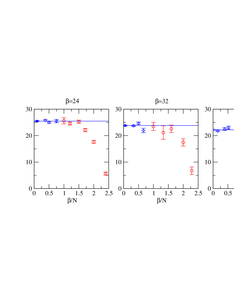
Figure 1: Finite-volume values for $\beta^{4}\{\langle 1-\frac{1}{3}\textrm{Tr}[P]\rangle_{a}-[c_{1}/\beta+c_{2}/\beta^{2}+c_{3}/\beta^{3}+c_{4}\ln\beta/\beta^{4}]\}$ as a function of the box size. The leftmost symbols indicate the infinite-volume estimates, obtained by fitting a constant to data in the range $\beta/N<1$ (blue diamonds). Points denoted by red circles are omitted from the extrapolation.

In Fig. 2 the infinite-volume extrapolated values of $\langle 1-\frac{1}{3}\textrm{Tr}[P]\rangle_{a}$ are plotted as a function of $1/\beta$.

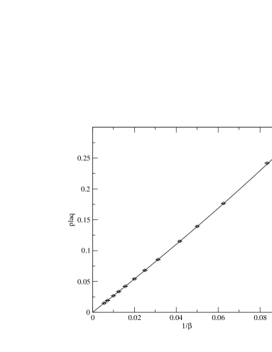
Figure 2: The plaquette expectation value plaq $\equiv\langle 1-\frac{1}{3}\textrm{Tr}[P]\rangle_{a}$ as a function of $1/\beta$. Statistical errors are much smaller than the symbol sizes. The solid line contains the four known terms $c_{1}/\beta+c_{2}/\beta^{2}+c_{3}/\beta^{3}+c_{4}\ln\beta/\beta^{4}$. The effect we are looking for is the difference between the data and the line.

A major difficulty in the simulations is the significance loss caused by the subtractions in eq. (7). The dominant term $c_{1}/\beta$ is about six orders of magnitude larger than the effect we are interested in, namely $\sim 1/\beta^{4}$, if $\beta\sim 100$. Therefore the relative error of our lattice measurements should be smaller than one part in a million. The effect of the subtractions is illustrated in Fig. 3.

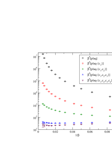
Figure 3: The significance loss due to the subtraction of divergent lattice contributions. Here again plaq $\equiv\langle 1-\frac{1}{3}\textrm{Tr}[P]\rangle_{a}$, and the symbols $c_{i}$ indicate which subtractions of eq. (2.7) have been taken into account.

Given the infinite-volume limits, we extrapolate the data to the continuum limit, $\beta\rightarrow\infty$. In Fig. 4 we show two functions: $\beta^{4}\{\langle 1-\frac{1}{3}\textrm{Tr}[P]\rangle_{a}-[c_{1}/\beta+c_{2}/\beta^{2}+c_{3}/\beta^{3}]\}$ and $\beta^{4}\{\langle 1-\frac{1}{3}\textrm{Tr}[P]\rangle_{a}-[c_{1}/\beta+c_{2}/\beta^{2}+c_{3}/\beta^{3}+c_{4}\ln\beta/\beta^{4}]\}$. Even the 4-loop logarithmic term is visible in the data. For $1/\beta\leq 0.01$ the significance loss grows rapidly and the error bars become quite large, so that these data points have little effect on the fit.

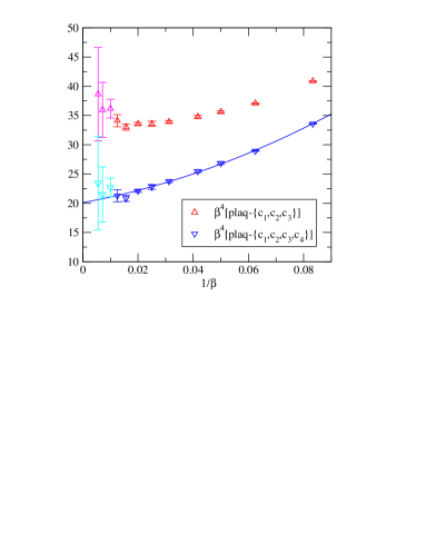
Figure 4: The infinite-volume extrapolated data. The effect of the 4-loop logarithmic divergence is to cause additional upwards “curvature” in the upper data set. The solid blue line gives the continuum extrapolation. Points with lighter colors have so large errors that they are insignificant as far as the fit is concerned.

The continuum extrapolation is carried out by fitting a function $d_{1}+d_{2}/\beta+d_{3}/\beta^{2}$ to the infinite-volume extrapolated data, from which all the divergences ($\{c_{1},c_{2},c_{3},c_{4}\}$) have been subtracted, in the range $0.01<1/\beta<0.10$. The fitted values are $d_{1}=20.0(7)$, $d_{2}=86(24)$ and $d_{3}=909(192)$ with $\chi^{2}/$dof$=5.8/6$. The error limits are the projections of the $68\%$ confidence level contour onto the various axes. The systematic errors from the effect of higher order terms are inside these errors.

Substituting this to eq. (7) we obtain the final result,

$$B_{\textrm{G}}+\left(\frac{43}{12}-\frac{157}{768}\pi^{2}\right)c_{4}^{\prime}=\frac{4\pi^{4}}{3^{6}}\times 20.0(7)=10.7(4).$$ (12)

4 Conclusions

We have studied the expectation value of the elementary plaquette in 3d pure SU(3) theory and outlined how the 3d vacuum energy density in the $\overline{\textrm{MS}}$ scheme can be extracted from it. However, to achieve this, the constant $c_{4}^{\prime}$ should be determined (cf. eqs. (3), (12)). This can be accomplished by a 4-loop matching computation, with the techniques discussed in ref. [11]. The full QCD pressure of order $g^{6}T^{4}$ can be obtained by a further 4-loop matching computation.

References

• [1] A.D. Linde, Infrared problem in thermodynamics of the Yang-Mills gas, Phys. Lett. B 96 (1980) 289.
• [2] D.J. Gross, R.D. Pisarski and L.G. Yaffe, QCD and instantons at finite temperature, Rev. Mod. Phys. 53 (1981) 43.
• [3] P. Ginsparg, First and second order phase transitions in gauge theories at finite temperature, Nucl. Phys. B 170 (1980) 388; T. Appelquist and R.D. Pisarski, High-temperature Yang-Mills theories and three-dimensional Quantum Chromodynamics, Phys. Rev. D 23 (1981) 2305.
• [4] K. Kajantie, M. Laine, K. Rummukainen and M. Shaposhnikov, Generic rules for high temperature dimensional reduction and their application to the Standard Model, Nucl. Phys. B 458 (1996) 90 [hep-ph/9508379].
• [5] E. Braaten and A. Nieto, Free energy of QCD at high temperature, Phys. Rev. D 53 (1996) 3421 [hep-ph/9510408].
• [6] A. Hietanen, K. Kajantie, M. Laine, K. Rummukainen and Y. Schröder, Plaquette expectation value and gluon condensate in three dimensions, JHEP 01 (2005) 013 [hep-lat/0412008].
• [7] Y. Schröder, Tackling the infrared problem of thermal QCD, Nucl. Phys. B (Proc. Suppl.)  129 (2004) 572 [hep-lat/0309112].
• [8] K. Kajantie, M. Laine, K. Rummukainen and Y. Schröder, The pressure of hot QCD up to $g^{6}\ln(1/g)$, Phys. Rev. D 67 (2003) 105008 [hep-ph/0211321].
• [9] U.M. Heller and F. Karsch, One loop perturbative calculation of Wilson loops on finite lattices, Nucl. Phys. B 251 (1985) 254.
• [10] H. Panagopoulos and A. Tsapalis, in preparation.
• [11] F. Di Renzo, A. Mantovi, V. Miccio and Y. Schröder, Four loop stochastic perturbation theory in 3d SU(3), Nucl. Phys. B (Proc. Suppl.)  129 (2004) 590 [hep-lat/0309111]; 3-d lattice Yang-Mills free energy to four loops, JHEP 05 (2004) 006 [hep-lat/0404003].