Interaction studies of a heavy-light meson-baryon system

Abstract

We study time correlation functions of operators representing heavy-light $K$–$\Lambda$ like systems at various relative distances $r$. The heavy quarks, one in each hadron, are treated as static. An anisotropic and asymmetric lattice is used with Wilson fermions. Our goal is to extract an adiabatic potential and thus learn about the physics of the five-quark system viewed as an hadronic molecule.

I Introduction

Lattice QCD studies of hadron-hadron interactions are the gateway to nuclear physics through first principles Savage (2005); Fiebig and Markum (2004). From a lattice simulation point of view the nucleon-nucleon interaction is probably the most challenging case. This is evident given the large spatial size of the deuteron, and in particular, the insight that the physics of the long-range strong interaction is driven mostly by the pion cloud Machleidt (1989). The latter may be taken as an indication that chiral symmetry and a full (unquenched) lattice action are high priorities for simulations aiming at quantitative results.

Aside from the above prominent case, however, interactions in other two-hadron systems are worth investigating as well, because this might lead to new insights into the structural features of some of the experimentally known baryon resonances Eidelman et al. (2004). In particular, we here ask if some of those may be understood as hadronic molecules, similar to the deuteron, but possibly with different physics of the interaction mechanisms in which quark and gluon degrees of freedom play a role. Prime candidates for such systems are pairs of hadrons containing one heavy quark each because, in the spirit of the Born-Oppenheimer approximation, the (slow) heavy quarks naturally serve to define the centers of two hadrons while the (fast) light quarks and gluons provide the physics of the interaction. Studies along those lines have been done before in the context of meson-meson and baryon-baryon systems Arndt et al. (2003); Michael and Pennanen (1999); Mihály et al. (1997).

We here report on the current status of interaction studies of a heavy-light meson-baryon (five-quark) hadron with the quantum numbers of an s-wave $K$–$\Lambda$ system. Because the static approximation is employed for the heavy-quark propagator, the total energy can be computed as a function of the relative distance $r$ between the heavy quarks. Thus an adiabatic (Born-Oppenheimer) potential $V_{a}(r)$ is extracted. This can be used to address the possibility of molecule-like structures.

II Simulation details

Two-hadron interpolating fields are constructed from standard local operators for the $K^{+}$ and the $\Lambda^{0}$ particles Montvay and Münster (1994) at relative distance $\vec{r}$ and projected to total momentum zero

$${\cal O}_{\alpha}(\vec{r};t)=V^{-1/2}\sum_{\vec{x}}\sum_{\vec{y}}\delta_{\textstyle\vec{r},\vec{x}-\vec{y}}\,K^{+}(\vec{x}t)\Lambda^{0}_{\alpha}(\vec{y}t)\,.$$ (1)

Here $V$ is the spatial lattice volume and $\alpha$ is a Dirac spinor index. Then, with

$$\bar{\cal O}_{\mu}(\vec{r};t)={\cal O}^{\dagger}_{\alpha}(\vec{r};t)\gamma_{4,\alpha\mu}$$ (2)

the correlation function

$$C=\langle{\cal O}_{\mu}(\vec{r};t)\bar{\cal O}_{\mu}(\vec{s};t_{0})\rangle-\langle{\cal O}_{\mu}(\vec{r};t)\rangle\langle\bar{\cal O}_{\mu}(\vec{s};t_{0})\rangle\,,$$ (3)

where $\vec{s}$ is the relative distance at the source, can be expressed in terms of fermion propagators. The flavor assignment $K^{+}\Lambda^{0}\sim\bar{s}u\,uds$ causes the separable term to vanish. Writing $H(\vec{x}t,\vec{y}t_{0})$ and $G(\vec{x}t,\vec{y}t_{0})$ for the heavy (s) and light (u,d) quark propagators, respectively, one obtains

$$C = \langle\sum_{\vec{y}}[H(\vec{y}t,\vec{y}+\vec{r}t)H(\vec{r}_{1}+\vec{s}t_{0},\vec{r}_{1}t_{0})-H(\vec{y}t,\vec{r}_{1}t_{0})H(\vec{r}_{1}+\vec{s}t_{0},\vec{y}+\vec{r}t)]$$

$$\rule{15.93048pt}{0.0pt}G(\vec{y}t,\vec{r}_{1}t_{0})[G(\vec{y}t,\vec{r}_{1}t_{0})G(\vec{y}+\vec{r}_{1}t,\vec{r}_{1}+\vec{s}t_{0})-G(\vec{y}t,\vec{r}_{1}+\vec{s}t_{0})G(\vec{y}+\vec{r}_{1}t,\vec{r}_{1}t_{0})]\rangle\,.$$

For clarity the rather involved color and spin index structure is not shown in (II). Also, translational invariance has been used to arrive at the above expression, and an arbitrary space site $\vec{r}_{1}$ was introduced in this context. A diagrammatic representation of (II) is shown in Fig. 1.

                                             

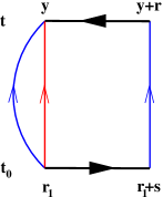
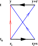
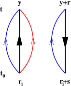
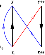
Figure 1: Diagrammatic representation of (II). Thick (black) lines indicate heavy-quark propagators, and thin (blue and red) lines depict light (u and d) quark propagators.

The heavy-quark propagators are employed in the static approximation. For (unimproved) Wilson fermions with hopping parameter $\kappa$ this means that the propagator is taken in the limit $\kappa\rightarrow 0$ , resulting in

$$H(\vec{x}t,\vec{y}t_{0})=\delta_{\textstyle\vec{x},\vec{y}}\;(2\kappa)^{t-t_{0}}\frac{1}{2}(1+\gamma_{4})\,\mathcal{U}^{\dagger}(\vec{x};t_{0}t)\,,$$ (5)

where $\mathcal{U}(\vec{x};t_{0}t)$ is the product of $SU(3)$ link variables along a straight line from $(\vec{x}t_{0})$ to $(\vec{x}t)$ Montvay and Münster (1994).

The distance $\vec{r}=0$ is rather special Michael and Pennanen (1999) because a color singlet operator, as realized by (1), can also be achieved by a “color twisted” version of (1) where quarks in $K^{+}$ and $\Lambda^{0}$ are combined into a color singlet. Because we do not consider color twisted operators in this work we restrict ourselves to non-zero relative distance. Thus, because $H(\vec{y}t,\vec{y}+\vec{r}t)\propto\delta_{\vec{r},\vec{0}}$ and $H(\vec{r}_{1}+\vec{s}t_{0},\vec{r}_{1}t_{0})\propto\delta_{\vec{s},\vec{0}}$, only the last two diagrams in Fig. 1 make a contribution to the correlation function for non-zero relative distance. By way of (5) those diagrams in Fig. 1 are proportional to $\delta_{\vec{y},\vec{r}_{1}}\delta_{\vec{r},\vec{s}}$. Thus (II) becomes

$$C = \delta_{\textstyle\vec{r},\vec{r}_{2}-\vec{r}_{1}}\;\langle H(\vec{r}_{1}t,\vec{r}_{1}t_{0})H(\vec{r}_{2}t_{0},\vec{r}_{2}t)$$

$$G(\vec{r}_{1}t,\vec{r}_{1}t_{0})[-G(\vec{r}_{1}t,\vec{r}_{1}t_{0})G(\vec{r}_{2}t,\vec{r}_{2}t_{0})+G(\vec{r}_{1}t,\vec{r}_{2}t_{0})G(\vec{r}_{2}t,\vec{r}_{1}t_{0})]\rangle\quad\mbox{for}\quad\vec{r}\neq 0\,,$$

where $\vec{r}_{2}$ is yet another arbitrary space site. We observe that sources at fixed spatial sites only are needed. However, an undesirable consequence of the static approximation is that the site sum $\sum_{\vec{y}}$ has vanished from (II) and thus is no longer working to improve statistics.

The final correlator we use is extended from (II) to a matrix by employing several levels $k=1\ldots K$ of operator smearing. The procedure amounts to replacing in (1) all light-quark fields $\psi,\bar{\psi}$ with smeared fields $\psi^{\{k\}},\bar{\psi}^{\{k\}}$. The computation of light-quark propagators thus requires various levels of smearing at the source and at the sink. We have used APE-style gauge field fuzzing Albanese et al. (1987) and Wuppertal fermion smearing Alexandrou et al. (1994) with common values for the strength parameters $\alpha=2.5$ and the number $k$ of iterations. No smearing, nor link variable fuzzing, was done for the heavy, static, quark fields in order to preserve spatial locality, i.e. the $\delta$ factor in (5). Thus, writing $\mathcal{O}\rightarrow\mathcal{O}^{\{k\}}=\mathcal{O}[\psi^{\{k\}},\bar{\psi}^{\{k\}}\ldots]$, the correlator (II) becomes a $K\times K$ matrix

$$C^{\,k\ell}(\vec{r};t,t_{0})=\langle\mathcal{O}{}^{\{k\}}_{\mu}(\vec{r};t)\,\bar{\mathcal{O}}{}^{\,\{\ell\}}_{\mu}(\vec{r};t_{0})\rangle\quad\mbox{with}\quad k,\ell=1\cdots K\,.$$ (7)

The expression for $C^{\,k\ell}$ in terms of quark propagators still has the form given by (II), however, light propagator elements are replaced with smeared ones, $G\rightarrow G^{\,k\ell}$, with appropriate smearing levels at source and sink. The correlation matrix (7) is hermitian by construction.

The lattice geometry is chosen as $L_{1}\times L_{2}\times L_{3}\times L_{4}=8\times 8\times 32\times 16$ with bare lattice constants $a_{1}=a_{2}=2a_{3}=2a_{4}$ in the respective directions. This choice of an asymmetric and anisotropic lattice provides a fine mass resolution, in t-direction, and the same spatial resolution for the adiabatic potential, as the static sources are placed along the z-direction. The positions of the latter are at $x=(5,5,n,3)$ with $n=1,2,3,4,8,11,13,17$, with $\vec{r}_{1,2}=(5,5,n)$ in reference to (II). In this way all possible relative distances $r=|\vec{r}|$ in the range $r=1\ldots 16$ can be obtained. Note that periodic boundary conditions, in the spatial directions, allow us to only utilize half of the extent of the lattice in z-direction.

We have used the Wilson plaquette action with Wilson fermions in a quenched simulation. The gauge field couplings in the $\mu$-$\nu$ planes and the hopping parameters in directions $\mu$ are given by, respectively,

$$\beta_{\mu\nu}=\beta\,\frac{a_{1}a_{2}a_{3}a_{4}}{(a_{\mu}a_{\nu})^{2}}\quad\mbox{and}\quad\kappa_{\mu}=\frac{\kappa}{a_{\mu}\frac{1}{4}\sum_{\nu=1}^{4}\frac{1}{a_{\nu}}}\,.$$ (8)

The simulation was done at $\beta=6.2$ with four values $\kappa=0.140,\,0.136,\,0.132,\,0.128$ of hopping parameters using a multiple mass solver Glässner et al. (1996).

III Analysis

The correlation matrix (7) is constructed with three smearing levels, $K=3$. It is then diagonalized separately on each timeslice $t$, using singular value decomposition. For asymptotic $t$ the largest eigenvalues correspond to the ground state of the two-hadron system. The maximum entropy method (MEM), as implemented in Fiebig (2002), is used to extract masses.

In order to set the physical mass scale the nucleon (N) and vector meson ($\rho$) masses are fit to the model $y=c_{1}+c_{2}x+c_{3}\ln(1+x)$, with $x=(am_{\pi})^{2}$, using the four available hopping parameters. Here $a=a_{3}=a_{4}$ is the common lattice constant in the $z$ and $t$ directions. The extrapolated values of $am_{N}$ and $am_{\rho}$, as $x\rightarrow 0$, are used to set the reduced mass of the $N$–$\rho$ system to its experimental value $m_{N\rho}=424$MeV. This gives $a=0.096$fm ($a^{-1}=2055$MeV) .

At the time of this writing the analysis is limited to 90 gauge configurations and to the largest value of the hopping parameter, $\kappa=0.140$. The corresponding results for the total energy $W$ are shown in Fig. 2a. The uncertainties are the (rms) widths of the spectral peaks emerging from the MEM analysis. Due to periodic boundary conditions the data points replicate for $r>16a$. For a preliminary analysis we use the simple model

$$aV(x)=\exp(-\alpha_{1}x^{2})(\alpha_{2}+\alpha_{3}x^{2}+\alpha_{4}x^{4})\quad\mbox{with}\quad x=r/a\,.$$ (9)

The fit to the data is then made using the periodic replication

$$aV_{L}(x)=\alpha_{0}+aV(x)+aV(L_{3}-x),\quad L_{3}=32\,,$$ (10)

of the model, which then has five parameters $\alpha_{0}\ldots\alpha_{4}$. Figure 2a shows the corresponding result. The plot in Fig. 2b represents (9) in terms of the physical scale, the adiabatic potential is $V_{a}(r)=V(r/a)$. Pending an anticipated increase of gauge configurations no error analysis for $V$ has been done at this time. However, error bands may be inferred from the uncertainties on the data points in Fig. 2a.

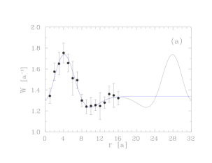
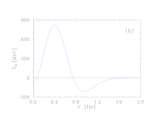
Figure 2: Total energy $W$ of the heavy-light $K$-$\Lambda$ like system versus the relative distance $r$ with MEM based uncertainties (a). The continuous lines represent fits with (9) and (10). The adiabatic potential $V_{a}$ is shown in physical units (b). Results are for $\kappa=0.140$.

The attractive dip of $V_{a}(r)$ at around $r\approx 0.8$–$1.2$fm, in Fig. 2b, may be significant enough to produce a molecule-like structure. As a first attempt to calculate phase shifts, we solve a standard non-relativistic scattering problem (Schrödinger equation) employing the computed adiabatic potential $V_{a}$ with several values $m_{R}$ for the reduced mass. For the latter we use the (experimental) reduced masses of the systems $K$–$\Lambda$, $D$–$\Lambda_{c}$, and $B$–$\Lambda_{b}$ from Eidelman et al. (2004). The resulting s-wave scattering phase shifts $\delta_{0}(p)$ are shown in Fig. 3. According to Levinson’s theorem ($\delta_{\ell}(0)-\delta_{\ell}(\infty)=n\pi$) the number $n$ of bound states is zero for the $K$–$\Lambda$ system. However, there is indication of an emerging resonance (rising phase shift) somewhat below $p=0.1a^{-1}$, or $E=62$MeV in terms of the relative kinetic energy. It should be kept in mind that Fig. 3 reflects a result at $m_{\pi}>0$ ($\kappa=0.140$). At present the strength of this feature as $m_{\pi}\rightarrow 0$ is an unresolved question. Also, relativistic effects are not taken into account. The latter are less significant for the $D$–$\Lambda_{c}$ and $B$–$\Lambda_{b}$ systems, respectively. Those appear to be bound by the adiabatic potential.

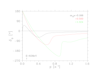
Figure 3: Scattering phase shifts (s-wave) for the $K$–$\Lambda$, $D$–$\Lambda_{c}$, and $B$–$\Lambda_{b}$ systems (black, red, and green, respectively) versus the, nonrelativistic, relative momentum $p$. The arrow indicates the relative kinetic energy for the $K$–$\Lambda$ system at $p=0.1a^{-1}$.

IV Assessment

Although in its present state the simulation is not conclusive, the results give a hint at potentially interesting physics. It appears conceivable that the known hadron mass spectrum may contain five-quark hadrons with a molecule-like structure. Our preliminary results would point to a resonant state with an excitation energy typical of a nuclear system, say $\approx 50\pm 50$MeV. As a possible candidate with the appropriate quantum numbers the N(1650) comes to mind Eidelman et al. (2004). Its mass lies just 40MeV above the $K$–$\Lambda$ threshold. However, we should caution that the extraction of masses typical for nuclear physics from a lattice simulation is difficult, because residual hadron-hadron interactions are, at least, one order of magnitude less that baryon rest masses. Therefore, awaiting the analysis with a reasonable number of gauge configurations, the above scenario should be considered an interesting possibility.

References

- Savage (2005) M. Savage, in 23rd International Symposium on Lattice Field Theory, 25-30 July 2005, Trinity College, Dublin, Ireland, PoS(LAT2005) (2005).
- Fiebig and Markum (2004) H. R. Fiebig and H. Markum, in Hadronic Physics from Lattice QCD, edited by A. M. Green (World Scientific, Singapore, 2004), vol. 9 of International Review of Nuclear Physics, chap. 4.
- Machleidt (1989) R. Machleidt, Adv. Nucl. Phys. 19, 189 (1989).
- Eidelman et al. (2004) S. Eidelman et al., Physics Letters B 592, 1+ (2004), URL http://pdg.lbl.gov.
- Arndt et al. (2003) D. Arndt, S. R. Beane, and M. J. Savage, Nucl. Phys. A726, 339 (2003), eprint nucl-th/0304004.
- Michael and Pennanen (1999) C. Michael and P. Pennanen (UKQCD), Phys. Rev. D60, 054012 (1999), eprint [http://arXiv.org/abs]hep-lat/9901007.
- Mihály et al. (1997) A. Mihály, H. R. Fiebig, H. Markum, and K. Rabitsch, Phys. Rev. D55, 3077 (1997).
- Montvay and Münster (1994) I. Montvay and G. Münster, Quantum Fields on the Lattice (Cambridge University Press, Cambridge, UK, 1994).
- Albanese et al. (1987) C. Albanese et al., Phys. Lett. B192, 163 (1987).
- Alexandrou et al. (1994) C. Alexandrou, S. Güsken, F. Jegerlehner, K. Schilling, and R. Sommer, Nucl. Phys. B414, 815 (1994), eprint [http://arXiv.org/abs]hep-lat/9211042.
- Glässner et al. (1996) U. Glässner, S. Güsken, T. Lippert, G. Ritzenhöfer, K. Schilling, and A. Frommer, Int. J. Mod. Phys. C7, 635 (1996), eprint [http://arXiv.org/abs]hep-lat/9605008.
- Fiebig (2002) H. R. Fiebig, Phys. Rev. D65, 094512 (2002), eprint [http://arXiv.org/abs]hep-lat/0204004.