Study of the systematic errors in the calculation of renormalization constants of the topological susceptibility on the lattice

Abstract:

We present a study of the systematic effects in the nonperturbative evaluation of the renormalization constants which appear in the field–theoretical determination of the topological susceptibility in pure Yang–Mills theory. The study is performed by computing the renormalization constants on configurations that have been calibrated by use of the Ginsparg-Wilson formalism and by cooling.

PoS(LAT2005)316

1 Introduction

There are several methods to evaluate the topological susceptibility $\chi$ in pure Yang–Mills theory on the lattice. Extracting this quantity for the $SU(3)$ gauge theory is crucial to understand the large mass of the $\eta^{\prime}$ meson in QCD [1, 2].

Some of the lastest results for $\chi^{1/4}$ obtained on the lattice are: $177(7)$ MeV by using cooling [3], $184(7)$ MeV by using cooling rounding the results to the closest integer [3], $191(5)$ MeV by counting fermionic zero modes [4] and $173.4(0.5)(1.2)$ MeV by the field–theoretical (or Pisa) method [5] (in this last number the statistical error and the error derived from the determination of the scale $\Lambda_{L}$ are shown separately).

Any comparison among these methods requires a good control of all sources of possible systematic errors. We present a progress report on a study about the systematic errors that are originated in the evaluation of multiplicative and additive renormalization constants that appear in the expression of the physical topological susceptibility $\chi$ in terms of the lattice one $\chi_{L}$. This relationship is [6, 7, 8]

$$\chi_{L}=Z^{2}a^{4}\chi+M\;,$$ (1)

where $Z$ and $M$ are multiplicative and additive renormalization constants respectively. To extract $\chi$ one has to know the value of $Z(\beta)$ and $M(\beta)$ where $\beta=6/g^{2}$, $g$ being the bare coupling constant. The lattice spacing $a(\beta)$ depends on the coupling $\beta$ in a way dictated by the lattice beta function.

The lattice susceptibility $\chi_{L}$ is calculated by using the definition

$$\chi_{L}\equiv\frac{\left\langle\left(Q_{L}^{(1)}\right)^{2}\right\rangle}{L^{4}}\;,$$ (2)

where $L^{4}$ is the spacetime volume and $Q_{L}^{(1)}$ is the 1–smeared topological charge [9].

2 Calculation of the renormalization constants

The renormalization constants $Z$ and $M$ are evaluated by using the heating method [10, 11]. Following the meaning of $Z$ [7, 8], we compute the average topological charge within a fixed topological sector. If we choose a topological sector of charge $n$ (any nonzero integer) then

$$Z=\frac{\left\langle Q_{L}^{(1)}\right\rangle\Big{|}_{Q=n}}{n}\;,$$ (3)

where the division by $n$ entails the requirement that $Q$ takes integer values ($Q$ here is defined by cooling). The brackets $\langle\cdot\rangle|_{Q=n}$ mean thermalization within the topological sector of charge $n$.

We start our algorithm with a classical configuration with topological charge $1$ ($Q=1$) and action $8\pi^{2}$ in appropriate units. Then we apply $80$ heat–bath steps of Cabibbo–Marinari updating [12] and measure $Q_{L}^{(1)}$ every $4$ steps. This set of $20$ measurements is called “trajectory”. After each measurement we apply 8 cooling steps to verify that the topological sector is not changed. We repeat this procedure to obtain a number of trajectories. For each trajectory we always discard the first few measurements because the configuration is not yet thermalized. Averaging over the thermalized steps (as long as the corresponding cooled configuration shows the correct background topological charge, $Q=1$ within a deviation $\delta$) yields $\left\langle Q_{L}^{(1)}\right\rangle\Big{|}_{Q=1}$. We estimate the systematic error that stems from the choice of $\delta$ as in [11].

As for the additive renormalization constant $M$ the procedure is quite analogous. We calculate $M=\chi_{L}|_{Q=0}\equiv\left\langle\left(Q_{L}^{(1)}\right)^{2}\right\rangle\Bigg{|}_{Q=0}/L^{4}$ in the zero topological charge sector (because within this sector the physical topological susceptibility $\chi$ vanishes). Single trajectories consist again of $80$ heat–bath steps with measurements every $4$ steps and cooling tests after each measurement. Thermalization of short distance fluctuations again requires discarding a few initial steps.

When a cooling test reveals that the corresponding configuration lies outside the correct topological sector ($Q=0$ for the calculation of $M$ and $Q=1$ for $Z$) then all points of the trajectory are discarded from that configuration onwards. In full QCD this event seldom happens [14, 15]; we work however in pure Yang–Mills theory where it happens more frequently.

An histogram containing the results of all cooling tests during a calculation of $Z(\beta=6.0)$ is shown in Fig. 1.

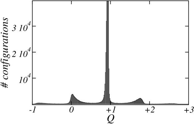
Figure 1: Histogram of background topological charge on all configurations obtained during a calculation of $Z(\beta=6.0)$ on a $16^{4}$ lattice.

It has been drawn from the set of all configurations measured within $25000$ trajectories: $25000\times 20=5\;10^{5}$ configurations. It is clear that in some cases the topological sector has moved towards topological charges different from $+1$. This occurs in the $30\%$ of all cases. Notice that the histogram is slanted: there are more configurations moving towards $Q=0$ than towards $Q=+2$ because the system tends to equilibrate around $Q=0$. Therefore if configurations within the wrong topological sector were not discarded, we would obtain a biased value for $Z$ (lower than the correct one).

When the additive renormalization $M$ is calculated, all configurations should lie in the $Q=0$ sector. If configurations that migrated outside this sector were not eliminated, the outcome for $M$ would be larger than the correct one as any departure from zero increases $M$ because it is proportional to the square of $Q_{L}^{(1)}$.

However the use of cooling to unravel the topological sector of a configuration may also destroy the unwanted instantons that alter the correct sector. In such a case we could not be able to discover that we are calculating the renormalization constants on wrong topological backgrounds. This problem comes about when the unwanted instanton is small and few cooling steps can destroy it rather easily. As described above, this circumstance distorts the extraction of $Z$ and $M$, yielding values for these constants that are lower ($Z$) or larger ($M$) than the correct ones. This is the source of systematic error that we want to quantify by checking the background topological charge by using a method different from cooling.

The counting of fermionic zero modes is a method to perform this check without modifying the configuration. Unfortunately it is much more demanding than cooling for quantifying the above described systematic effect.

3 Zero modes counting checks

The net number of zero modes $n_{+}-n_{-}$ is obtained by counting the level crossings in the spectrum of the Wilson–Dirac operator as the fermion mass $m$ varies [16, 17, 18]. This method was used in [18, 19] to calculate the topological charge. We use an accelerated conjugate gradient algorithm [20] to extract the lowest eigenvalues of the Wilson–Dirac operator.

This technique looks ambiguous because there can be level crossings all along the interval of masses where the gap is closed. If we stop counting crossings at some mass inside the interval, in general the resulting topological charge depends on the choice of this mass. It is shown [18] that physical results do not depend strongly on the choice of this mass. In particular, instantons representing crossings that are close to $a\,m=2$ (the endpoint of allowed masses) have a size of a few lattice spacings. These are precisely the instantons that most probably could evade the cooling test. Therefore we show results for $a\,m=2$.

We want to calculate both $M$ and $Z$ at some fixed value of the lattice coupling $\beta$. The topological charge background will be checked both by cooling and by counting of fermionic zero modes and the final results compared. Any difference between these final results can be interpreted as an estimate of the systematic error. At this writing we have completed $50$ trajectories for $M$ at $\beta=6.0$ on a $12^{4}$ lattice for the quenched $SU(3)$ theory. We show the partial results deduced from this limited set of trajectories. In Fig. 2 the average among trajectories is shown for the two methods of checking. As for the cooling, the configuration was considered as belonging to the right sector $Q=0$ within a deviation $|\delta|=0.3$. We show only data after the $16$th heat–bath step (previous steps are irrelevant because the quantum fluctuations are not yet thermalized). The points in grey color are the average of all data in all trajectories. They are

$$M_{\rm cooling}=0.66(4)\;10^{-5}\;,\qquad\qquad M_{\rm fermionic}=0.72(4)\;10^{-5}\;.$$ (4)

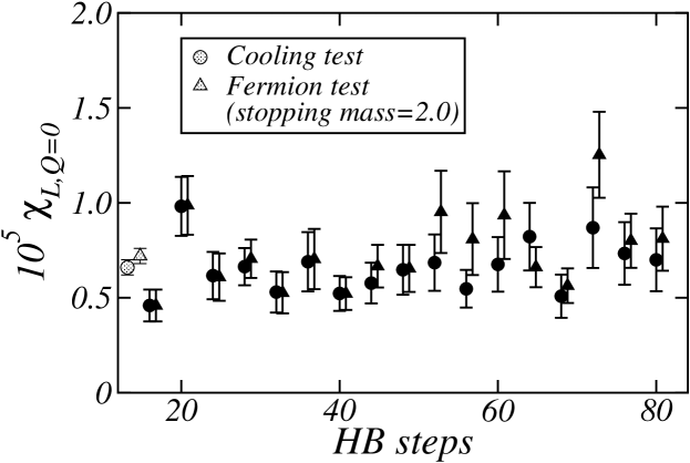
Figure 2: Average on a set of $50$ trajectories for the calculation of $M$ by using both cooling (circles) and fermionic level crossing counting (triangles) as checks of the topological background. The level cross counting stopped at $a\,m=2$.

In Fig. 3 the number of configurations used for the average in Fig. 2 at each step is displayed. Ideally the number of configurations should be $50$, however due to the discarding of configurations with a wrong topological charge background, this number decreases as a function of the step. Notice that this decrease is steeper for the cooling although it is supposed that some instantons escape the cooling check while they should be netted by the counting of zero modes (mainly with the stopping mass fixed at $a\,m=2$). The plot depends little on the choice of $\delta$, ($\delta=0.1$ or $0.5$ yield similar data). The fact that the result for $M$ obtained with cooling (see (4)) tends to be lower than the results obtained by counting zero modes seems to indicate a better performance of cooling in discovering wrong charge configurations. However our error bars are still too large to be able to draw any clean conclusions from the data. We plan to improve the statistics roughly by one order of magnitude both for $M$ and $Z$.

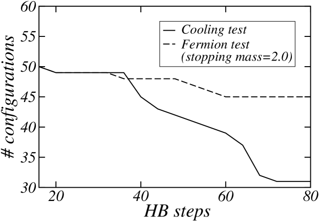
Figure 3: Number of configurations used for the average in Fig. 3 as a function of the heat–bath step for cooling checks (straight line) and fermionic level crossing counting (dashed line).

References

- [1] E. Witten, Nucl. Phys. B156 (1979) 269.
- [2] G. Veneziano, Nucl. Phys. B159 (1979) 213.
- [3] B. Lucini, M. Teper, U.Wenger, Nucl. Phys. B715 (2005) 461.
- [4] L. Del Debbio, L. Giusti, C. Pica, Phys. Rev. Lett. 94 (2005) 032003.
- [5] B. Allés, M. D’Elia, A. Di Giacomo, Phys. Rev. D71 (2005) 034503.
- [6] W. Zimmermann Lectures on Elementary Particles and Quantum Field Theory in 1970 Brandeis School, edited by S. Deser, M. Grisaru, H. Pendleton.
- [7] M. Campostrini, A. Di Giacomo, H. Panagopoulos, Phys. Lett. B212 (1988) 206.
- [8] B. Allés, E. Vicari, Phys. Lett. B268 (1991) 241.
- [9] C. Christou, A. Di Giacomo, H. Panagopoulos, E. Vicari, Phys. Rev. D53 (1996) 2619.
- [10] B. Allés, M. Campostrini, A. Di Giacomo, Y. Gündüç, E. Vicari, Phys. Rev. D48 (1993) 2284.
- [11] B. Allés, M. D’Elia, A. Di Giacomo, Nucl. Phys. B494 (1997) 281, Erratum: ibid B679 (2004) 397.
- [12] N. Cabibbo, E. Marinari, Phys. Lett. B119 (1982) 387.
- [13] K. Wilson, Phys. Rev. D10 (1974) 2445.
- [14] B. Allés, G. Boyd, M. D’Elia, A. Di Giacomo, E. Vicari, Phys. Lett. B389 (1996), 107.
- [15] B. Allés et al., Phys. Rev. D58 (1998), 071503.
- [16] R. Narayanan, H. Neuberger, Nucl. Phys. B443 (1995) 305.
- [17] H. Neuberger, Phys. Rev. D61 (2000) 085015.
- [18] R. G. Edwards, U. M. Heller, R. Narayanan, Nucl. Phys. B535 (1998) 403.
- [19] L. Del Debbio, C. Pica, JHEP 02 (2004) 003.
- [20] B. Bunk, K. Jansen, M. Lüscher, H. Simma, Conjugate gradient algorithm to compute the low–lying eigenvalues of the Dirac operator in lattice QCD, unpublished report (1994); T. Kalkreuter, H. Simma, Comput. Phys. Commun. 93 (1996) 33.