Observations on discretization errors in twisted-mass lattice QCD

Abstract

I make a number of observations concerning discretization errors in twisted-mass lattice QCD that can be deduced by applying chiral perturbation theory including lattice artifacts. (1) The line along which the PCAC quark mass vanishes in the untwisted mass-twisted mass plane makes an angle to the twisted mass axis which is a direct measure of $O(a)$ terms in the chiral Lagrangian, and is found numerically to be large; (2) Numerical results for pionic quantities in the mass plane show the qualitative properties predicted by chiral perturbation theory, in particular an asymmetry in slopes between positive and negative untwisted quark masses; (3) By extending the description of the “Aoki regime” (where $m_{q}\sim a^{2}\Lambda_{\rm QCD}^{3}$) to next-to-leading order in chiral perturbation theory I show how the phase transition lines and lines of maximal twist (using different definitions) extend into this region, and give predictions for the functional form of pionic quantities; (4) I argue that the recent claim that lattice artifacts at maximal twist have apparent infrared singularities in the chiral limit results from expanding about the incorrect vacuum state. Shifting to the correct vacuum (as can be done using chiral perturbation theory) the apparent singularities are summed into non-singular, and furthermore predicted, forms. I further argue that there is no breakdown in the Symanzik expansion in powers of lattice spacing, and no barrier to simulating at maximal twist in the Aoki regime.

I Introduction

Twisted mass fermions tm at maximal twist FR1 ; FR2 ; FR3 are presently under intensive study both with simulations and theoretical methods. The standard application involves two degenerate quarks, and this is the theory considered here. The long distance physics (vacuum and pionic properties) of twisted mass lattice QCD with two degenerate flavors (tmLQCD) can be studied using the methods of effective field theory, allowing a systematic dual expansion in the quark mass, $m_{q}$, and the lattice spacing, $a$, in which non-perturbative effects are parameterized by a priori unknown low energy constants (LECs) ShSi ; Noam ; Oliver . The resulting theory is called twisted-mass chiral perturbation theory (tm$\chi$PT) MS . Its consequences in the vacuum and pionic sector have been worked out to next-to-leading order (NLO) in the regime with $m_{q}\mathrel{\hbox to0.0pt{\lower 3.0pt\hbox{$\mathchar 536\relax$}\hss}\raise 2.0pt\hbox{$\mathchar 318\relax$}}a\Lambda^{2}$ (the “generic small mass” or GSM regime ) AB04 ; ShWu2 , and at leading order (LO) in the regime with $m_{q}\sim a^{2}\Lambda^{3}$ (the “Aoki” regime) Mun04 ; Scor04 ; AB04 ; ShWu1 ; ShWu2 . Here $\Lambda$ is a scale of the order of the QCD scale, $\Lambda_{\rm QCD}$.

The present paper is a collection of observations that follow from tm$\chi$PT concerning discretization errors in tmLQCD. On the practical side, I point out in sec. II some new applications of results contained in Ref. ShWu2 . In particular, I describe how the observed difference between two methods of determining maximal twist that are being used in simulations can be understood using tm$\chi$PT. This difference provides a direct measure of the size of discretization errors, or equivalently a measure of the LECs related to such errors. I also point out the relationship of these methods to a third (theoretically interesting but apparently less practical) method proposed in Ref. ShWu2 .

In sec. III I note that the dependence of physical quantities on the untwisted quark mass at fixed twisted quark mass gives another set of measures of the size of discretization errors, some of which are related by tm$\chi$PT at NLO. These results are contained in Ref. ShWu2 , but have not been compared to the available numerical data, and I think it is useful to provide illustrative plots of the expected types of dependence.

When making these plots the question arises as to how to extend them into the Aoki regime, which is the regime in which there are phase transitions caused by competition between quark mass effects and those due to discretization errors. Previous studies, in Refs. Mun04 ; Scor04 ; AB04 ; ShWu1 ; ShWu2 , worked to LO in this regime, and here I extend these results to NLO. This extension, described in sec. IV, turns out to require only one non-trivial additional low-energy coefficient. The results allow one to see how the phase transition lines, which are linear at LO, can become curved at NLO, and similarly how the lines of maximal twist using different definitions behave. These results may be amenable to numerical investigation, but, in any case, are of theoretical interest in understanding the relationship between different definitions of twist angle and critical mass. I also point out that, while a classical analysis is sufficient when working to NLO in the Aoki regime, extension to next-to-next-to-leading order (NNLO) requires the inclusion of loop effects.

My final topic, discussed in sec. V, is the conclusions of Ref. FMPR . It is argued in FMPR that, if one makes an estimate of the critical mass that has an error of size $a\Lambda^{2}$, then, when working at maximal twist, physical correlation functions contain apparently infrared (IR) divergent discretization errors proportional to $(a/m_{\pi^{0}}^{2})^{2k}$, with $k\geq 1$ an integer. Such errors, while consistent with automatic $O(a)$ improvement, would restrict one to working with $m_{q}>a\Lambda^{2}$, and suggest a breakdown of the Symanzik expansion Symanzik for smaller quark masses. It is then argued that, either by using an “optimal” choice of critical mass, or using a non-perturbatively improved quark action, these IR divergent errors at maximal twist can be reduced in size to $a^{2}(a^{2}/m_{\pi^{0}}^{2})^{k}$. In this way the bound on the quark mass is reduced to $m_{q}>a^{2}\Lambda^{3}$, i.e. one can work in the GSM regime but not in the Aoki regime.

My observation is that the IR divergences are an indication of expanding around the wrong vacuum in the presence of large perturbation. Using tm$\chi$PT one can sum these corrections to all orders and obtain a finite and smooth prediction for the dependence of physical quantities on the underlying untwisted and twisted quark masses. Indeed, this is precisely what was done previously in Refs. AB04 ; ShWu2 . I argue further that there is no breakdown of the Symanzik expansion, suitably interpreted, and no barrier to working at maximal twist in the Aoki regime.

These considerations do not, however, invalidate the conclusion of Ref. FMPR that one should use an appropriate “optimal” choice of critical mass to reduce the size of discretization errors. This was proposed previously using tm$\chi$PT in Refs.  AB04 ; ShWu2 , and the criteria for determining the optimal choice agree. My observation here is that, since tm$\chi$PT is built upon the Symanzik expansion used by Ref. FMPR , the result concerning optimal critical masses had to agree. In fact, tm$\chi$PT goes beyond the Symanzik expansion by adding non-perturbative information concerning spontaneous chiral symmetry breaking. The only additional assumption that one has to make is that the effective field theory framework is valid Weinberg ; Leutwyler .

It is useful to keep in mind during the subsequent discussions the physical values of quark masses that correspond to the different regimes. If one takes $a^{-1}=2\;$GeV (a relatively small lattice spacing for present dynamical simulations) and $\Lambda\approx\Lambda_{\rm QCD}\approx 300\;$MeV, then $a\Lambda^{2}$ (the size of quark masses in the GSM regime) and $a^{2}\Lambda^{3}$ (the size in the Aoki regime) are about $45$ and $7\;$MeV respectively. Since we are interested in calculating with light quark masses varying from $m_{\rm strange}\approx 80-100\;$MeV down toward $m_{\rm light}\approx 3-4\;$MeV, most simulations will be done in the GSM regime, with a significant tail entering the Aoki regime. Thus it is important to understand both regimes in detail.

In this paper I work in the “twisted basis” in which the tmLQCD action is

$$S^{L}_{F}=\;\sum_{x}\bar{\psi_{l}}(x)\Big{[}\frac{1}{2}\sum_{\mu}\gamma_{\mu}(\nabla^{\star}_{\mu}+\nabla_{\mu})-\frac{r}{2}\sum_{\mu}\nabla^{\star}_{\mu}\nabla_{\mu}+m_{0}+i\gamma_{5}\tau_{3}\mu_{0}\Big{]}\psi_{l}(x),\,.$$ (1)

Here $\psi_{l}$ is the dimensionless bare lattice field, $\mu_{0}$ is the bare twisted mass and $m_{0}$ the bare untwisted mass. The coefficient of the Wilson term, $r$, is typically set to unity in simulations; the considerations that follow hold, however, for any $O(1)$ choice of this coefficient. Maximal twist is obtained by setting $m_{0}$ to an estimate of its critical value $m_{c}$ (which, as will be seen, can depend on $\mu_{0}$). The determination of $m_{c}$ is a key issue in tmLQCD, and the topic of much of the discussion which follows. I only note here that this is a non-trivial issue as no symmetry is restored when $m_{0}=m_{c}$. By contrast, setting $\mu_{0}=0$ restores parity and flavor symmetries, and physical quantities are symmetrical under $\mu_{0}\to-\mu_{0}$.

I use the twisted basis, rather than the more continuum-like “physical basis”, used for example in Ref. FMPR , since the twisted basis is that usually used in simulations, allowing a more direct connection to the numerical data. It is also the basis used in the tm$\chi$PT calculations of Ref. ShWu2 , which I use extensively.

The physical twisted and untwisted masses are $\mu=Z_{\mu}\mu_{0}/a$ and $m=Z_{m}(m_{0}/a-m_{c})$, respectively, with $Z_{\mu}=1/Z_{P}$ and $Z_{m}=1/Z_{S}$ renormalization constants. The physical quark mass is then $m_{q}=\sqrt{\mu^{2}+m^{2}}$, and to work at maximal twist requires setting $m=0$ (i.e. setting $m_{0}=am_{c}$). The accuracy with which $m_{c}$ must be determined in order to maintain automatic $O(a)$ improvement depends on how close to the chiral limit one is working. If $m_{q}\gg a\Lambda^{2}$, then discretization errors are small, and the error in $m_{c}$ can be of $O(a)$. This possibility is part of the topic of sec. V. In the GSM regime, one must incorporate $O(a)$ discretization effects into $m_{c}$ AB04 ; ShWu2 , and thus reduce the error to $O(a^{2})$. To work in the Aoki regime and maintain automatic $O(a)$ improvement requires the uncertainty in $m_{c}$ to be further reduced, to $O(a^{3})$ AB04 ; ShWu2 . Following Ref. FMPR , I refer to choices of critical mass which are accurate to $O(a^{3})$ as “optimal”, and denote them by $m^{\prime}_{c}$ (and the resulting untwisted quark mass by $m^{\prime}$). I discuss these choices in secs. II and III. One noteworthy choice of $m_{c}$, which, as stressed in Ref. AB04 , is not optimal, is given by the position where the pion mass vanishes (an end-point of the Aoki phase, if present). This differs from optimal choices by $O(a^{2})$. Finally, if one works at NLO in the Aoki regime, it is natural, as shown in sec. IV, to incorporate an $O(a^{3})$ shift into $m_{c}$. I denote the resulting critical mass and untwisted physical quark mass by $m^{\prime\prime}_{c}$ and $m^{\prime\prime}$, respectively. The uncertainty in $m^{\prime\prime}_{c}$ turns out to be of $O(a^{5})$. The fact that only odd powers of $a$ appear has been noted also in Ref. FMPR .

So as not to clutter the notation with too many “primes”, I use the same (unprimed) symbol for $m_{q}$ in each regime, although it is defined using the untwisted quark mass appropriate to the given regime. Thus, for example, in the Aoki regime, $m_{q}=\sqrt{\mu^{2}+m^{\prime\prime 2}}$.

The variables $m_{0}/a$ and $\mu_{0}/a$ (or $m$ and $\mu$, or $m^{\prime}$ and $\mu$, etc.) map out what I will refer to as the “mass plane”. The origin in this plane is defined to be where $\mu_{0}=0$ and $m_{0}/a$ is set to the critical value appropriate to the regime of interest. With the definitions given above, $m_{q}$ is then the distance from the origin. Once $m_{c}$ is estimated, one possible definition of the twist angle (that which relates most directly to that used in the continuum) is the angle relative to the positive untwisted mass axis. This angle depends on the choice of critical mass, but I refer to it as $\omega_{0}$ in all regimes. It is most useful in the GSM regime, where it is defined by

$$\omega_{0}\equiv\tan^{-1}(\mu/m^{\prime})\,.$$ (2)

In the Aoki regime, at NLO, one replaces $m^{\prime}$ with $m^{\prime\prime}$.

Finally, I collect the notation I use for low energy coefficients (LECs) in tm$\chi$PT, largely taken over from Ref. ShWu2 . At leading order, there are two continuum LECs: $f$, the decay constant in the chiral limit normalized to $f_{\pi}=132\;$MeV, and $B_{0}$, defined so that $m_{\pi}^{2}=2B_{0}m_{q}$. For quark masses renormalized at $2\;$GeV in the $\overline{{\rm MS}}$ scheme, $B_{0}\approx 2.5\;$GeV. It is then convenient to introduce $\hat{\mu}=2B_{0}\mu$ and $\hat{m}=2B_{0}m$ and $M=\sqrt{\hat{\mu}^{2}+\hat{m}^{2}}$ so that, at LO, $m_{\pi}^{2}=M$. At NLO in the continuum, there are the standard Gasser-Leutwyler coefficients, the $L_{i}$ GLoneloop . Discretization errors introduce other LECs. At LO in the GSM regime, there is a single constant $W_{0}$, which determines the $O(a)$ shift in $m_{c}$ ShSi ; Noam . In particular, defining $\hat{a}=2W_{0}a$, then the shifted untwisted mass is $\hat{m}^{\prime}\equiv 2B_{0}m^{\prime}=\hat{m}+\hat{a}$, and $m_{\pi}^{2}=M^{\prime}\equiv\sqrt{\hat{\mu}^{2}+(\hat{m}^{\prime}){}^{2}}$. Discretization errors of NLO in the GSM regime are determined by the dimensionless constants $W$, $W_{10}$, $\widetilde{W}$, and $W^{\prime}$ Noam ; Oliver ; ShWu2 . It is convenient to introduce the following quantities:

$$\delta_{W}\equiv\frac{16\hat{a}(W+W_{10}/4)}{f^{2}}\,,\ \ \delta_{\widetilde{W}}\equiv\frac{16\hat{a}(\widetilde{W}+W_{10}/2)}{f^{2}}\,,\ \ w^{\prime}\equiv\frac{16\hat{a}^{2}W^{\prime}}{f^{2}}\,.$$ (3)

$\delta_{W}$ and $\delta_{\widetilde{W}}$ give dimensionless measures of the size of discretization errors in physical quantities, while the mass-squared $w^{\prime}$ appears additively in the result for the pion mass-squared. Note $\delta_{W}$ and $\delta_{\widetilde{W}}$ are linear in $a$, while $w^{\prime}$ is quadratic. Further LECs enter at NLO in the Aoki regime, and will be defined in sec. IV.

II Comparing definitions of maximal twist

As noted in the introduction, one must use a non-perturbative method of sufficient accuracy in order to determine when one is at maximum twist. This section concerns the relation between two methods being used in present simulations [which I refer to as methods (i) and (ii)] and their relationship to a third method [method (iii)] proposed in Ref. ShWu2 . Throughout this section I assume that the quark masses are in the GSM regime.

My observations are summarized in Fig. 1. The line in the mass-plane defined by method (i) (in which the PCAC mass is set to zero) makes an angle $\delta\omega$ to the twisted mass direction [and thus, by construction, to the line defined by method (ii)]. This angle is proportional to the lattice spacing, and to one combination of the LECs describing discretization errors. It can be determined from present simulations, and the results show that this discretization error is not as small as one might hope, since it is determined by a scale $\Lambda\approx 0.7\;$ GeV rather than by $\Lambda\approx\Lambda_{\rm QCD}$. I also observe, following Ref. ShWu2 , that method (iii), previously argued to be difficult to implement in practice, is actually equivalent to method (ii) in the GSM regime (and thus has already been used).

Both method (i) and (ii) are based on the continuum result that, at maximal twist, charged axial currents in the twisted basis correspond to physical vector currents, and thus should have vanishing coupling to physical charged pions. It is useful to introduce a definition of twist angle incorporating this result:

$$\tan\omega_{A}=\frac{\langle 0|V^{2}_{\mu}|\pi^{1}\rangle}{\langle 0|A^{1}_{\mu}|\pi^{1}\rangle}\,,$$ (4)

where the currents are in the twisted basis, and the superscripts are adjoint $SU(2)$ indices. This angle is denoted $\omega$ in Ref. ShWu2 , but I add the subscript “A” here for clarity. Maximal twist can then be defined by $\omega_{A}=\pm\pi/2$, corresponding to Farchioni04B

$$\langle 0|A^{1}_{\mu}|\pi^{1}\rangle=0\,,$$ (5)

Note that the charged pions can be unambiguously created by the local pseudoscalar density (which is invariant under the axial transformation that rotates between twisted and physical bases). The condition (5) is equivalent to setting the PCAC mass (defined in sec. III below) to zero.

The two methods apply the condition (5) in different ways. In method (i) the condition is enforced for each choice of $\mu_{0}$ by varying $m_{0}$ ShWu2 ; Lewis . This leads to a curve in the mass plane which one follows as $\mu_{0}$ is reduced. To good approximation this curve is found to be a straight line for the masses used in present simulations Lewis ; Jansen05 . This method is sometimes called the parity-conservation definition, but I do not use this name as parity is not restored along the line it defines at non-zero lattice spacing [and the name could equally well be applied to method (iii) discussed below]. Method (ii) defines the critical mass by extrapolating the curve along which the condition (5) holds to $\mu_{0}=0$ Jansen05 . The resulting simulations are then done holding $m_{0}$ fixed at this value, with $\mu_{0}$ varying. This method is also that proposed in Ref. FMPR . Figure 1 illustrates the difference between the two methods.

Figure 1: Illustration of different methods for working at maximal twist. See text for description [method (iv) is discussed in sec. V]. The arrows represent the direction one moves to approach the chiral limit (which occurs at $\mu_{0}=0$). The plot represents the GSM regime in which $m_{q}\sim a$. The Aoki regime, in which $m_{q}\sim a^{2}$ is represented by the shaded region. It is discussed in sec. IV. The angle $\delta\omega$ is defined to be positive for the situation shown in the Figure.

The curve defined in method (i) is displayed in Fig. 7 of Ref. Lewis and Fig. 1 of Ref. Jansen05 . (In both figures the $m_{0}$ and $\mu_{0}$ axes are interchanged compared to Fig. 1, and in the second figure the vertical axis is $1/\kappa$ rather than $m_{0}=1/(2\kappa)-4$.) These are results from quenched simulations, but I will not rely on the details of these results, instead assuming only that the following features are general and continue to hold in unquenched simulations: (1) the curves are almost linear for small $\mu$ (roughly for $\mu_{0}/a\mathrel{\hbox to0.0pt{\lower 3.0pt\hbox{$\mathchar 536\relax$}\hss}\raise 2.0pt\hbox{$\mathchar 316\relax$}}30\;$MeV); and (2) they approach the $\mu_{0}=0$ axis at an angle that differs from $\pi/2$. Indeed this difference (denoted by $\delta\omega$ in Fig. 1) is significant: approximately $0.8$ radians for $\beta=5.7$ Jansen05 , $0.5$ for $\beta=5.85$ and $0.35$ for $\beta=6$ Lewis .

The first observation I want to make is that the result $\delta\omega\neq 0$ is a prediction of tm$\chi$PT, and that the value of $\delta\omega$ is a direct measure of $O(a)$ discretization errors. This follows from results contained in Ref. ShWu2 . In particular, method (i) is the same as using the canonical definition of maximal twist suggested in Ref. ShWu2 . It follows from setting $\omega_{A}=\pi/2$ in eq. (58) of that work (where, recall, $\omega_{A}$ is denoted $\omega$) that the line of maximal twist in method (i) lies at an angle

$$\omega_{0}=\pi/2-\delta\omega\,,\qquad\delta\omega=-(Z_{m}/Z_{\mu})\delta_{W}+O(a^{2})\,,$$ (6)

relative to the origin where $\mu_{0}=0$ and $m_{0}/a=m^{\prime}_{c}$ [i.e. $\omega_{0}$ is defined as in eq. (2)]. Here $\delta_{W}$ is defined in eq. (3) above, and the factor of $Z_{m}/Z_{\mu}=Z_{P}/Z_{S}$ arises because the predictions of Ref. ShWu2 are given in terms of physical masses, rather than the bare masses used in Fig. 1. An implication of the result (6) is that the line defined in method (i) extrapolates to a critical mass which includes the $O(a)$ shift, confirming that it is an optimal choice. It then follows that method (ii) corresponds to setting $\omega_{0}=\pi/2$.

The most noteworthy feature of eq. (6) is that the effect is linear in $a$. The angle $\delta\omega$ is an example of a quantity which is not automatically improved at maximal twist (as discussed more extensively in Ref. ShWu2 ). The result (6) also incorporates the result that using different lattice axial currents in the criterion (5) leads to different results for $\delta\omega$. For example, using an improved current with $c_{A}\neq 0$ instead of an unimproved current can be seen to lead to a change in $\delta\omega$ proportional to $ac_{A}$. This effect enters through the dependence of $\delta_{W}$ on the LEC $W_{10}$, for $W_{10}$ itself depends on the choice of current. Note that if one uses non-perturbatively improved Wilson fermions (which sets $W=0$ as discussed in Ref. ShWu2 ) and a non-perturbatively improved axial current (which sets $W_{10}=0$), then $\delta\omega$ is predicted to vanish at $O(a)$. In this case the difference between methods (i) and (ii) appears at next-to-next-to-leading order (NNLO) in tm$\chi$PT, arising, for example, from a contribution proportional to $a\mu^{2}\bar{\psi}\psi$ in the Symanzik effective action. This latter term gives the critical mass a quadratic dependence on $\mu_{0}^{2}$. The resulting small curvature can in fact be seen in the quenched results discussed above, particularly in the results at the largest lattice spacing Jansen05 .

It should be stressed that a non-zero value for $\delta\omega$ does not contradict automatic improvement as long as it is of $O(a)$. Contributions to physical quantities linear in $a$ are necessarily also proportional to $\delta\omega$, so the overall discretization error remains of $O(a^{2})$. Indeed, as stressed in Refs. FR1 ; ShWu2 , there is an intrinsic, irreducible ambiguity in the twist angle: different criteria, equally good in the continuum limit, lead to results differing at $O(a)$ at non-vanishing lattice spacing. In fact, one can define maximal twist as lying along any line in the mass plane whose angle satisfies $\omega_{0}=\pi/2+O(a)$, where the $O(a)$ offset is arbitrary. Note that for all such lines the quark mass is $m_{q}=\mu[1+O(a^{2})]$, and thus, to NLO accuracy, one can use $m_{q}=\mu$.

The above-mentioned curvature in the maximal twist line of method (i) allows one to estimate the size of the ambiguity in the resulting critical mass. The NNLO curvature means that, when extrapolating to $\mu=0$ from $\mu\sim O(a)$, the angle $\delta\omega$ has an error of $O(a^{2})$. This leads to an error in the intercept $m^{\prime}_{c}$ of size $O(a^{3})$, consistent with the size predicted by tm$\chi$PT and noted in the introduction.

For practical applications it is important to study $\delta\omega$ as an indicator of the size of discretization errors. One expects $|\delta\omega|=a\Lambda$, with $\Lambda$ a scale lying somewhere in the range from $\Lambda_{\rm QCD}\approx 300\;$MeV to $\Lambda_{\chi}=2\sqrt{2}f\approx 1.2\;$GeV. For the $\beta=6$ results of Ref. Lewis ($\delta\omega\approx 0.35$ at $a^{-1}\approx 2\;$GeV) one finds $\Lambda\approx 0.7\;$GeV (assuming $Z_{\mu}/Z_{m}\approx 1$). The results at the other lattice spacings are roughly consistent with this scale, or, to put it another way, are roughly consistent with the expected linear dependence on $a$. One should not expect more than a rough consistency because there is additional implicit logarithmic dependence on $a$, entering, for example, through the factor $Z_{\mu}/Z_{m}$, as well as NNLO terms of $O(a^{2})$.

Given the result for $\delta\omega$, one can very roughly estimate the size expected for the $O(a^{2})$ errors in physical quantities—they should be approximately be of relative size $(\delta\omega)^{2}$. This is approximate because different LECs and numerical factors enter for each quantity. Nevertheless, if one uses it as a guide, one expects $O(a^{2})$ errors of relative size $\sim 10\%$ for $a^{-1}\approx 2\;$GeV. It should be borne in mind, however, that changes to the gluon and fermion actions, as well as changing from quenched to unquenched simulations, will change the size of the LECs and thus the discretization errors.

It is interesting to ask what happens to the relationship between methods (i) and (ii) for negative $\mu_{0}$. In this case, it follows from eq. (58) of Ref. ShWu2 with $\omega=-\pi/2$ that the figure is symmetric under reflection in the $m_{0}$ axis. In fact, this follows from the invariance of the underlying lattice theory under parity transformation combined with a change of sign of $\mu_{0}$. Thus the line determined by the condition (5) appears to have a cusp at the $\mu_{0}=0$ axis. How this extends into the Aoki regime is one of the questions addressed below in sec. IV.

Knowing the combination of LECs appearing in $\delta\omega$ allows one to predict other quantities using tm$\chi$PT. In particular, one of the parity violating axial form factors of the pion [the $p_{1}$ term in eq. (91) of Ref. ShWu2 at maximal twist and for $q^{2}\to 0$] depends only on $\delta_{W}$. Thus, as long as one knows $Z_{P}/Z_{S}$, one can predict this form factor up to NNLO corrections.

I now turn to my second observation about the relationship between methods for determining maximal twist. A third definition of the twist angle is given in Ref. ShWu2 , and denoted $\omega_{P}$. It is based on requiring that the physical scalar density does not create the neutral pion from the vacuum. Method (iii) for determining maximal twist is defined by setting $\omega_{P}=\pi/2$, and is equivalent to requiring that $\langle 0|P^{3}|\pi^{0}\rangle=0$, where $P^{3}$ is the neutral pseudoscalar density in the twisted basis. In Ref. ShWu2 it was argued that this method would be difficult to implement in practice, since the required matrix elements involve disconnected quark contractions. My observation here (which follows from eq. (98) of Ref. ShWu2 ) is that at maximum twist [defined using any of methods (i-iii)]

$$\omega_{P}=\omega_{0}+O(a^{2})=\pi/2+O(a^{2})\qquad\textrm{(maximal twist).}$$ (7)

In other words, up to NNLO corrections, methods (ii) and (iii) are the same. Thus it turns out not to be difficult to implement method (iii) in the GSM regime. The generalization of this result to the Aoki regime is discussed below.

III Comparing tm$\chi$PT expressions to simulations

In this short section I point out that existing simulation data exhibit qualitative features predicted by tm$\chi$PT, and that by doing more detailed fits one could over-determine the LECs associated with discretization errors. I illustrate these points by showing plots of physical quantities for a choice of LECs roughly consistent with the numerical results of Ref. Farchioni04B . For most of this section I work in the GSM regime, although the plots extend into the Aoki regime, and use results from the following section. I assume that an optimal critical mass $m^{\prime}_{c}$ has been determined, i.e. that one knows the critical mass with errors of $O(a^{3})$. I then consider the functional dependence of physical quantities on the untwisted quark mass $m^{\prime}$ at fixed values of the twisted quark mass $\mu$.

As explained in Ref. FR1 (and extended into the GSM regime in Refs. AB04 ; ShWu2 ; FMPR ) $O(a)$ errors in physical quantities can be canceled by “mass averaging”, i.e. by suitably averaging the results at $(m^{\prime},\mu)$ and $(-m^{\prime},-\mu)$ (which corresponds to averaging $\pm m_{q}$ in the physical basis used in Ref. FR1 ). Here the term “suitable” indicates that, for quantities with negative $R_{5}$ parity (defined in Ref. FR1 ), the term at $(-m^{\prime},-\mu)$ must be included with a negative sign FR1 . Physical masses and matrix elements, however, have positive $R_{5}$ parity. One can change the average to one between $(m^{\prime},\mu)$ and $(-m^{\prime},+\mu)$ by doing, for example, a parity transformation on the second term. This transformation, which I refer to as “twisted parity”, is equivalent to $\omega\to-\omega$ in the physical basis. As discussed in Ref. FR1 , it does not effect physical quantities, but can lead to a sign change in certain correlation functions. The net result is that for physical quantities one cancels $O(a)$ errors by averaging over $(m^{\prime},\mu)$ and $(-m^{\prime},\mu)$ with relative positive signs, while for other quantities one must determine the relative sign of the two terms on a case-by-case basis. Two examples used below are the PCAC mass and the expectation value $\langle P^{3}\rangle$. The former has odd $R_{5}$ parity, but even twisted parity (at $\vec{p}=0$), and so requires a relative minus sign for the two contributions. The latter has odd $R_{5}$ and twisted parities, and so the average has relative positive signs.

The point I want to make here is that the contributions that are canceled by the mass average described above are also of interest, for they provide a measure of discretization errors, and allow tests of tm$\chi$PT at NLO. These non-continuum parts can be picked out using

$$AS(Q)=\frac{Q(m^{\prime},\mu)-(-)^{p}Q(-m^{\prime},\mu)}{Q(m^{\prime},\mu)+(-)^{p}Q(-m^{\prime},\mu)}\,,$$ (8)

where $Q$ is the quantity of interest, and $(-)^{p}$ is the product of its $R_{5}$ and twisted parities. The name refers to “antisymmetric”, since for most quantities (all those considered here except $m_{\rm PCAC}$) $AS$ is the antisymmetric part. Using the results of Ref. ShWu2 , I find

$$AS(m_{\pi^{\pm}}^{2}) = 2\ AS(\langle 0|P^{\mp}|\pi^{\pm}\rangle)=AS(\langle\pi|S^{0}|\pi\rangle)=(m^{\prime}/m_{q})(2\delta_{W}-\delta_{\widetilde{W}})+O(a^{2})\,,$$

$$AS(f_{A}) = (m^{\prime}/m_{q})\,\delta_{\widetilde{W}}/2+O(a^{2})\,,$$

$$AS(m_{\rm PCAC}) = (m_{q}/m^{\prime})\,\delta_{W}+O(a^{2})\,,$$ (9)

$$AS(\langle P_{3}\rangle) = O(a^{2})\,,$$

$$AS(m_{\pi^{0}}^{2}-m_{\pi^{\pm}}^{2}) = O(a)\,.$$

Here $f_{A}$ is the usual pion decay constant, and $m_{\rm PCAC}$ is defined in the following section. I stress that these results hold in the GSM regime, but not in the Aoki regime. One sees that tm$\chi$PT relates the “antisymmetries” in the various quantities. In particular, if $\delta_{W}$ has been determined using the angle $\delta\omega$ as described in the previous section, then only one additional parameter ($\delta_{\widetilde{W}}$) is needed to describe all seven quantities in eq. (9). This assumes that the ratio $Z_{P}/Z_{S}$ is known so that bare mass ratios can be converted into those of physical masses.

One peculiar feature of the results in (9) is the appearance of $m_{q}/m^{\prime}=1/\cos\omega_{0}$ in the result for $m_{\rm PCAC}$. By contrast, all the other results that are non-vanishing at NLO are proportional to $\cos\omega_{0}$, and thus vanish when $m^{\prime}=0$. The divergence at $m^{\prime}=0$ in $AS(m_{\rm PCAC})$ results from the fact that the average is not taken with respect to the position at which $m_{\rm PCAC}$ vanishes (which, as seen in the previous section, occurs along a line with $\omega_{0}=\pi/2-\delta\omega$ and not along the line $\omega_{0}=\pi/2$). In any case, the result becomes invalid when $\cos\omega_{0}$ becomes of $O(a)$, i.e. when one enters the Aoki regime, so that one does not in fact reach the divergence.

Figure 5 of Ref. Farchioni04B shows plots of $m_{\pi^{\pm}}^{2}$ and $m_{\rm PCAC}$ as a function of $m_{0}$ at $\mu_{0}=0$ and $0.01$. These results are from dynamical simulations with a lattice spacing of $a^{-1}\approx 1\;$GeV. In physical units (and assuming that $Z_{S}\approx Z_{P}\approx 1$) the twisted quark mass is thus $0$ and $10\;$MeV, while $m^{\prime}$ lies in the range $-100\;{\rm MeV}\mathrel{\hbox to0.0pt{\lower 3.0pt\hbox{$\mathchar 536\relax$}\hss}\raise 2.0pt\hbox{$\mathchar 316\relax$}}m^{\prime}\mathrel{\hbox to0.0pt{\lower 3.0pt\hbox{$\mathchar 536\relax$}\hss}\raise 2.0pt\hbox{$\mathchar 316\relax$}}50\;$MeV. Since $a\Lambda_{\rm QCD}^{2}\approx 90\;$MeV and $a^{2}\Lambda_{\rm QCD}^{3}\approx 30\;$MeV, the results lie in both Aoki and GSM regimes. Two features of these results are relevant here. First, there is a clear lack of symmetry in the results for $m_{\pi^{\pm}}^{2}$, and of antisymmetry in $m_{\rm PCAC}$, i.e. the quantities $AS(m_{\pi^{\pm}}^{2})$ and $AS(m_{\rm PCAC})$ are non-vanishing. Thus it would be interesting to do a more detailed fit to determine them. Second, since a significant fraction of the data points lie in the Aoki region, as shown by the evidence for a first order phase transition, a comprehensive fit requires a functional form that is valid in both GSM and Aoki regimes. The expressions in eq. (9) do not suffice, for they are valid only in the GSM regime.

The following section is devoted to providing functional forms valid in both regimes. Since the “antisymmetry” arises at NLO in the GSM regime, a consistent form must be valid also at NLO in the Aoki regime. In fact, once one works at NLO, it may be that the best approach is to simply fit to the full formulae for both positive and negative quark masses rather than use the “antisymmetries” directly.

I close this section by illustrating the forms that result from the joint NLO analysis in GSM and Aoki regimes. I use the following parameters, which are roughly chosen to match the behavior seen in Ref. Farchioni04B . The LECs describing discretization errors are set to $\delta_{W}=\delta_{\tilde{W}}=-0.3$, $2w^{\prime}=(0.25\;{\rm GeV})^{2}$, and $W_{3,3}=0$ ($W_{3,3}$ being the additional non-trivial LEC needed at NLO in the Aoki region, as discussed in the following section). In addition I set the continuum LECs (the $L_{i}$ of Gasser and Leutwyler) to zero and drop chiral logarithms. Although both these contributions are of NLO in the GSM region, and thus should be included for consistency, they do not contribute to the “antisymmetries”. Furthermore, they are of NNLO in the Aoki regime. Note that if I define scales by $\delta_{W}=-a\Lambda_{W}$, $\delta_{\widetilde{W}}=-a\Lambda_{\widetilde{W}}$, and $2w^{\prime}=a^{2}\Lambda_{w^{\prime}}^{4}$, and use $a^{-1}=1\;$GeV, the parameters I use correspond to $\Lambda_{W}=\Lambda_{\widetilde{W}}=300\;$MeV, and $\Lambda_{w^{\prime}}=500\;$MeV, which are reasonable values for the scales of discretization errors. The choice $W_{3,3}=0$ is made for simplicity. Taking $w^{\prime}>0$ implies that one is in the first-order scenario of Ref. ShSi , consistent with the numerical results. The quantity $\sqrt{2w^{\prime}}=250\;$MeV is then approximately the minimum pion mass. See Fig. 4(b) for a sketch of the phase diagram.

Figure 2 shows the forms of $m_{\pi^{\pm}}^{2}$ for $\mu$ fixed at $0$, $10$, $15$ and $25\;$MeV, and Fig. 3 shows the corresponding plots for $m_{\rm PCAC}$. In both figures the left-hand plot shows the results primarily in the GSM regime, while the right-hand plot zooms in on the Aoki region. Within the GSM regime, the mass $m^{\prime\prime}$ (defined in the following section) is equivalent, at NLO, to the mass $m^{\prime}$ used in this section. The prediction of eq. (9) that the “antisymmetries” should be independent of $\mu$ holds to good approximation for $|m^{\prime\prime}|\mathrel{\hbox to0.0pt{\lower 3.0pt\hbox{$\mathchar 536\relax$}\hss}\raise 2.0pt\hbox{$\mathchar 318\relax$}}50\;$MeV. The values of $AS$ for both quantities asymptote at large $|m^{\prime\prime}|$ to $-0.3$, roughly the values one obtains from the data of Ref. Farchioni04B .

I discuss the features in the Aoki regime in the next section. I only note here that the first order phase transition can be seen in the jumps for $\mu=0$ and $10\;$MeV. The end-point of the transition is for $\mu=w^{\prime}/B_{0}=12.5\;$MeV (as discussed in the following section) so that the lines with $\mu=15$ and $25\;$MeV pass above the transition.

Figure 2: $m_{\pi^{\pm}}^{2}$ as a function of $m^{\prime\prime}$ for fixed $\mu=0,0.01,0.015,0.025$, for the parameter set described in the text. Here $m^{\prime\prime}$ is the NLO quark mass in the Aoki regime, defined in eq. (12). For the GSM regime [i.e. most of fig. (a)] $m^{\prime\prime}$ is equivalent to $m^{\prime}$ at NLO accuracy. All quantities are in units of appropriate powers of GeV. The curves in (a) can be identified from the enlargement (b): the lines decrease in thickness as $\mu$ increases, with the $\mu=0.025$ curve dashed.

Figure 3: $m_{\rm PCAC}$ as a function of $m^{\prime\prime}$, with parameters and legend as in Fig. 2.

IV The Aoki regime at NLO

In this section I extend the tm$\chi$PT analysis in the Aoki region to NLO. The motivation for making this extension is twofold. First, it allows one to see what happens in detail to the phase transition line, and to the lines of maximal twist, as one enters the Aoki region. In particular, it clarifies the size and parametric form of the errors that are made in different schemes for determining maximal twist. Second, it provides NLO results that can be used consistently in the Aoki and GSM regimes.

The main results of this section are that a NLO analysis in the Aoki regime requires only one non-trivial additional LEC, and that this leads to changes in the phase diagram, as summarized in Fig. 4. These changes are small, proportional to $a^{3}$ as compared to the size of the phase boundary ($\sim a^{2}$), but lead to new effects which might be measurable, e.g. curvature in the phase boundary, and a discontinuity in the pion mass across the boundary. I also determine the lines of maximal twist, and results for a number of physical pionic quantities, both at NLO. These are of theoretical interest, and may be needed to describe the results of numerical simulations. Finally, I describe what happens to the phase diagram if the gauge action is tuned so as to reduce the size of the LEC which determines the phase structure at LO from $\sim a^{2}$ to $\sim a^{3}$.

In the Aoki regime, LO terms are of size $m_{q}\sim a^{2}$ (terms linear in $a$ having been absorbed into the quark mass), and NLO contributions are suppressed by a power of $a$. Thus NLO terms are of size $m_{q}a$, $p^{2}a$ and $a^{3}$. The first two are also of NLO in the GSM regime, and thus are already included in the NLO chiral Lagrangian of Ref. ShWu2 . The $a^{3}$ terms are new. Using the properties of $SU(2)$, I find that there are two independent terms:

$${\cal L}_{\chi}^{(a^{3})}=-\frac{W_{3,1}}{f^{2}}\left[\mathrm{Tr}(\hat{A}^{\dagger}\hat{A})\mathrm{Tr}(\hat{A}^{\dagger}\Sigma)+h.c.\right]-\frac{W_{3,3}}{f^{2}}\left[\mathrm{Tr}(\hat{A}^{\dagger}\Sigma)^{3}+h.c.\right]\,,$$ (10)

where $h.c.$ indicates hermitian conjugate, and $\hat{A}$ is the spurion associated with discretization errors, which is set to $\hat{a}$ times the identity matrix. The new LECs, $W_{3,1}$ and $W_{3,3}$, are dimensionless.

Recalling the form of the leading order mass term

$$-\frac{f^{2}}{4}\mathrm{Tr}(\chi^{\prime\dagger}\Sigma)+h.c.\,,$$ (11)

where $\chi^{\prime}=\hat{m}^{\prime}+i\tau_{3}\hat{\mu}$ is the mass spurion, we see that the $W_{3,1}$ term can be absorbed by a redefinition of $\chi^{\prime}$ and $\hat{m^{\prime}}$:

$$\chi^{\prime}\longrightarrow\chi^{\prime\prime}=\chi^{\prime}+\frac{8\hat{a}^{3}W_{3,1}}{f^{4}}\equiv\hat{m}^{\prime\prime}+i\tau_{3}\hat{\mu}\,.$$ (12)

This is equivalent to an $O(a^{3})$ shift in $m_{c}$. Since one does not know $m_{c}$ a priori, this shift does not increase our ignorance. All the formulae quoted above, and in Ref. ShWu2 , hold to their stated accuracy with $\chi^{\prime}$ replaced by $\chi^{\prime\prime}$ (and thus $M^{\prime}$ replaced with $M^{\prime\prime}=\sqrt{{\hat{m}^{\prime\prime}}{}^{2}+\hat{\mu}^{2}}$ and using $\tan\omega_{0}=\mu/m^{\prime\prime}$).

Thus there is only one non-trivial new term to include in the analysis. Before describing how this changes the LO results, I want to comment on redundancy in the LECs. In Ref. ShWu2 , it was shown that the LEC $W_{10}$ could be set to zero by a change of variables, as long as other LECs were adjusted accordingly. This implied that, if one kept $W_{10}$ in the analysis, the results would depend only on certain linear combinations of LECs. Extending this analysis to the $O(a^{3})$ terms, I find that the contributions of the two new constants to physical quantities must appear in combinations $2W_{3,3}+W_{3,1}$ and $W_{3,3}-32W^{\prime}W$. I have used this to check the results given below, but, to simplify expressions, I have set $W_{10}$ to zero having made these checks.

Now I turn to the results. My aim is to map out the phase structure at fixed $a$ as a function of $m^{\prime\prime}$ and $\mu$, and to determine NLO expressions for physical quantities throughout this mass plane. Note that, although $m^{\prime\prime}$ is not known a priori, one can use the results given here to determine $m^{\prime\prime}$ a posteriori. Where appropriate I will include contributions which, while of NNLO in the Aoki regime, are of NLO in the GSM regime, and thus are needed for a complete, continuous description within the mass plane.

I begin with the determination of the expectation value, $\Sigma_{m}$, of the pion field $\Sigma\in SU(2)$. This is the value which minimizes the classical potential, which is here

$$\frac{V_{\chi}}{f^{2}}=-(c_{m}\hat{m}^{\prime\prime}+s_{m}\hat{\mu})(1+c_{m}\delta_{W})-c_{m}^{2}w^{\prime}-c_{m}^{3}w_{3}+O(a^{4})\,,$$ (13)

where I use

$$c_{m}=\mathrm{Tr}(\Sigma_{m})/2\,,\ \ \textrm{and}\ \ s_{m}=-i\mathrm{Tr}(\Sigma\tau_{3})/2\,,$$ (14)

and define the useful quantity

$$w_{3}=\frac{16\hat{a}^{3}W_{3,3}}{f^{4}}\,.$$ (15)

The range of the variables is $-1\leq c_{m},s_{m}\leq 1$, with the constraint $-\sqrt{1-c_{m}^{2}}\leq s_{m}\leq\sqrt{1-c_{m}^{2}}$. For $\hat{\mu}\neq 0$, the linear dependence of $V_{\chi}$ on $s_{m}$ implies that $s_{m}$ is pushed to one or other end of its allowed range, so that $s_{m}^{2}+c_{m}^{2}=1$. This implies that $\Sigma_{m}$ lies in the $\tau_{3}$ direction. For $\hat{\mu}=0$ (the Wilson axis), one can choose the expectation value to lie in the $\tau_{3}$ direction. Thus from now on I set $\Sigma_{m}=\exp(i\omega_{m}\tau_{3})$, so that $s_{m}=\sin\omega_{m}$ and $c_{m}=\cos\omega_{m}$.

In the Aoki region, the LO potential, obtained by setting $\delta_{W}=w_{3}=0$, has been analyzed in Refs. Mun04 ; Scor04 ; ShWu1 . There are two scenarios depending on the sign of $w^{\prime}$, as shown (including NLO effects) in Fig. 4. For $w^{\prime}<0$, a transition line lies along the Wilson axis, within which parity and flavor are spontaneously broken (the Aoki phase Aoki ), with endpoints at $\hat{m}^{\prime\prime}=\mp 2w^{\prime}$. This I call the “Aoki-phase scenario”. For $w^{\prime}>0$, there is a first order transition line along the $\mu$ axis with second-order endpoints at $\hat{\mu}=\pm 2w^{\prime}$. This I call the “first-order scenario”.

The extension of this analysis to NLO is straightforward in principle. The extra terms are, by assumption, small, and do not change the qualitative features of the two scenarios. They do, however, lead to small changes in the positions of the transition lines and the predictions for other quantities.

I consider first the Aoki-phase scenario ($w^{\prime}<0$). Along the Wilson axis, the $-c_{m}\hat{m}^{\prime\prime}$ term in the potential ensures that $c_{m}$ is forced to one or other end of its allowed range for large enough $|\hat{m}^{\prime\prime}|$: $c_{m}={\rm sgn}(\hat{m}^{\prime\prime})$. The phase transition occurs when the other terms cancel this force, i.e. when $dV_{\chi}/dc_{m}(c_{m}=\pm 1)=0$. This occurs at

$$\hat{m}^{\prime\prime}=\mp 2w^{\prime}-3w_{3}+4w^{\prime}\delta_{W}+O(a^{4})\qquad\textrm{(Aoki-phase endpoints)}\,.$$ (16)

The first term on the r.h.s. is the LO result, which is of $O(a^{2})$. The next two terms are the $O(a^{3})$ corrections, which lead to a shift in the phase transition line, but do not change its length. Of course, to measure this shift requires knowing where the origin is, and I return to this point below. Within the Aoki phase, the identity component $c_{m}$ varies continuously from $+1$ to $-1$ (in a way which can be determined, if needed, by minimizing $V_{\chi}$). I only note here that the expectation value points purely in $\tau_{3}$ direction ($c_{m}=0$) when $\hat{m}^{\prime\prime}=0$, which is not the mid-point of the transition line (unlike at LO). As at LO, the charged pions are massless in the Aoki phase, with the neutral pion also massless at the end points.

The changes at NLO are more significant in the first-order scenario. There is no symmetry which requires the transition to lie parallel to the $\mu$ axis once NLO terms are included. To begin I consider the position of the transition line on the Wilson axis. The transition occurs when the two minima at $c_{m}=\pm 1$ have equal energy. Because the $w_{3}$ term in $V_{\chi}$ is an odd function of $c_{m}$, this occurs not at $\hat{m}^{\prime\prime}=0$ (the LO result) but at $\hat{m}^{\prime\prime}=-w_{3}$. For $\hat{m}^{\prime\prime}$ greater than (less than) this value, $c_{m}=+1$ ($-1$).

This analysis is easily generalized off the Wilson axis. At LO, the first-order transition is present at $\hat{m}^{\prime\prime}=0$ if $|\hat{\mu}|<2w^{\prime}$. The LO potential has equal minima at $c_{m}=\pm c_{m}^{0}=\pm\sqrt{1-(s_{m}^{0})^{2}}$, both having $s_{m}=s_{m}^{0}=\hat{\mu}/(2w^{\prime})$. The two minima coalesce into second-order endpoints at $\hat{\mu}=\pm 2w^{\prime}$. At NLO, the terms odd in $c_{m}$ give opposite contributions at the two minima, and one must adjust $\hat{m}^{\prime\prime}$ to make their energies equal. To the order I work, $\hat{m}^{\prime\prime}$ can be determined by enforcing $V_{\chi}(c_{m}=c_{m}^{0})=V_{\chi}(c_{m}=-c_{m}^{0})$. From this it follows that the transition is shifted to

$$\hat{m}^{\prime\prime}=-w_{3}+(w_{3}-2w^{\prime}\delta_{W})\left(\frac{\hat{\mu}}{2w^{\prime}}\right)^{2}+O(a^{5})\qquad(\textrm{1st order line:}\ |\hat{\mu}|\leq 2w^{\prime})\,.$$ (17)

The transition line is thus a quadratic function of $\mu$, which maintains the symmetry under $\mu\to-\mu$ while being smooth at $\mu=0$. The value of $\hat{\mu}$ at the end-points is unchanged from LO, aside from NNLO corrections of $O(a^{4})$ discussed below. For a given $\hat{\mu}$, however, the error in $\hat{m}^{\prime\prime}$ turns out to be of $O(a^{5})$, rather than the naively expected $O(a^{4})$. Finally I note that the NLO terms shift the angle $\omega_{m}$ at the transition line from the LO value by

$$\delta\omega_{m}=\omega_{m}-\omega_{m}^{0}=(\delta_{W}-w_{3}/w^{\prime})(\hat{\mu}/[2w^{\prime}])+O(a^{2})\,.$$ (18)

This $O(a)$ shift is in the same direction on both sides of the transition, so the resulting values of $c_{m}$ on the two sides differ in magnitude: $c_{m}=\pm c_{m}^{0}-(\delta\omega_{m})\,s_{m}^{0}$. This leads to the discontinuity in $m_{\pi}^{2}$ at the transition, as shown in Fig. 2 and discussed below.

To understand the size of the uncertainty in the position of the end-points it is useful to display the form of the potential there. The considerations are identical for both end-points, and I choose to consider that at positive $\mu$. Setting $\hat{\mu}=2w^{\prime}$ and $\hat{m}^{\prime\prime}=-2w^{\prime}\delta_{W}$ [from eq. (17)], one has

$$\frac{V_{\chi}}{f^{2}}=\frac{w^{\prime}c_{m}^{4}}{4}+(w^{\prime}\delta_{W}-w_{3})c_{m}^{3}+2w^{\prime}\delta_{W}^{2}c_{m}^{2}\qquad\textrm{(1st order endpoint).}$$ (19)

I have dropped terms of higher order than quartic in $c_{m}$, as they would be subleading in the following discussion. At LO, only the first term on the r.h.s. contributes. It has a minimum at $c_{m}=0$, and corresponds to the end-point since the curvature vanishes. At NLO, the value of $\hat{m}^{\prime\prime}$ has been chosen by the criterion given above so that $c_{m}=0$ remains a stationary point of the potential. $c_{m}=0$ does not, however, correspond to an end-point, for there is a non-vanishing quadratic term at $c_{m}=0$ (with coefficient $\propto a^{4}$). Furthermore, for some values of the LECs, the cubic term leads to a second stationary point with $c_{m}\sim a$. To move to the actual end-point, one must shift $\hat{\mu}$ and, in general, $\hat{m}^{\prime\prime}$. For example, the quadratic term can be canceled by a shift of size $\delta\hat{\mu}\sim a^{4}$, because $\delta V_{\chi}\propto\delta\hat{\mu}(1-c_{m}^{2}/2+\dots)$. It can be shown that a similarly sized shift in $\hat{\mu}$, as well as a shift $\delta\hat{m}^{\prime\prime}\sim a^{5}$, will also remove the second minimum, if present.

A NLO calculation does not, however, control the size of these shifts. This is because there are neglected higher order contributions to the potential which are of the same size as those in eq. (19) when $c_{m}\sim a$. For example, there will be NNLO and higher order contributions to the classical potential of the form $\delta V_{\chi}\sim a^{4}c_{m}^{2}+a^{5}c_{m}$, depending on additional unknown LECs. These, like the terms in (19), are of $O(a^{6})$ when $c_{m}\sim O(a)$, and thus compete with NLO terms. In particular, the term linear in $c_{m}$ leads to an unknown shift $\delta\hat{m}^{\prime\prime}\sim a^{5}$, and the quadratic term to a shift $\delta\hat{\mu}\sim a^{4}$.

In addition, loop contributions to the effective potential enter at the same order. Flavor-conserving four-pion vertices of LO (and thus proportional to $p^{2}$ or $m_{q}$) give rise to quadratic terms in the potential of the form $\delta V_{\chi}\sim c_{m}^{2}m_{\pi}^{4}\ln(m_{\pi})\sim a^{4}c_{m}^{2}$. The latter equality follows because, for charged pions, $m_{\pi}^{2}\sim a^{2}$ at the end-points. There are also flavor-violating four-pion vertices of the form $a^{2}s_{m}^{2}W^{\prime}\vec{\pi}\cdot\vec{\pi}\pi_{3}^{2}$ (see Ref. ShWu2 ), and these also lead to $\delta V_{\chi}\sim c_{m}^{2}a^{2}m_{\pi}^{2}\ln m_{\pi}\sim a^{4}c_{m}^{2}$. Finally, there are tadpole diagrams involving three-pion vertices. These vertices have been given in Ref. ShWu2 in the GSM regime. In the Aoki regime they become

$$f{\cal L}_{\chi}^{3\pi}=-\delta_{\tilde{W}}\pi_{3}\partial_{\mu}\vec{\pi}\cdot\partial_{\mu}\vec{\pi}+\frac{s_{m}\hat{m}^{\prime\prime}-c_{m}\hat{\mu}}{2}\pi_{3}\vec{\pi}\cdot\vec{\pi}\,.$$ (20)

Noting that the coefficient of the second term is of $O(a^{3})$ at the end-points, I find that the contributions to the potential are of the form

$$\delta V_{\chi}^{\rm tad}\sim c_{m}(am_{\pi}^{4}\ln m_{\pi}+a^{3}m_{\pi}^{2}\ln m_{\pi})\sim a^{5}c_{m}\,,$$ (21)

and thus of the same size as the higher order terms in the classical potential for $c_{m}\sim a$. Clearly extending the calculation beyond NLO will be challenging.

A corollary of the previous discussion is that, close to the end point, the NLO calculation does not control the shift $\delta\omega_{m}$, since higher order terms contribute with the same size as LO and NLO terms. For the result (18) to be valid, the distances from an end-point must satisfy $\delta\hat{\mu}\gg a^{4}$ or $\delta\hat{m}^{\prime\prime}\gg a^{5}$. Furthermore, as one approaches the end-points the rate of convergence of the chiral expansion slows. For example, if one moves a distance $\delta\hat{m}^{\prime\prime}\sim a^{3}$ from the end-point, then one can show that $c_{m}\sim a^{1/3}$. It follows that each higher order is suppressed by a relative factor of $\sim a^{2/3}$, rather than $\sim a$.

The results for the phase structure are summarized in Fig. 4. The circles around the end-points emphasize that the chiral expansion breaks down in their vicinity, as just discussed. Note that, since the origin of $\hat{m}^{\prime\prime}$ is not known, in the Aoki-phase scenario one can, at this stage, only determine $w^{\prime}$ from the length of the phase region, while in the first-order scenario one can determine both $w^{\prime}$ (from the length in the $\mu$ direction), and $w_{3}-2w^{\prime}\delta_{W}$ (from the extent of the phase line in the $\hat{m}^{\prime\prime}$ direction).

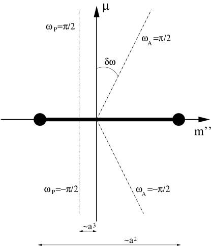
(a) Aoki-phase

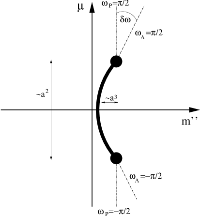
(b) First-order

Figure 4: Illustration of phase structure and lines of maximal twist at NLO in the Aoki regime for both Aoki-phase and first-order scenarios. The solid lines indicates first-order transition lines, with the solid circles being second-order end-points. Both masses $m^{\prime\prime}$ and $\mu$ range up to values of $O(a^{2})$ in this figure, with other features (the asymmetry in the phase line in the Aoki-phase, the offset of the $\omega_{P}=\pm\pi/2$ lines, and the horizontal extent of the phase-line in the first-order scenario) being of $O(a^{3})$. See the text for more details. The angle $\delta\omega$ is the same as that in Fig. 1.

I now turn to results for other physical quantities. To do so, one needs to know the value of $\omega_{m}$ for a general position in the mass plane. This is determined by solving

$$0=\frac{1}{f^{2}}\frac{dV_{\chi}}{d\omega_{m}}=s_{m}\hat{m}^{\prime\prime}-c_{m}\hat{\mu}+2c_{m}s_{m}w^{\prime}+(2c_{m}s_{m}\hat{m}^{\prime\prime}+[s_{m}^{2}-c_{m}^{2}]\hat{\mu})\delta_{W}+3c_{m}^{2}s_{m}w_{3}+O(a^{4})\,,$$ (22)

and choosing the solution with minimal energy. In practice, for general values of the parameters, and away from the phase boundaries, one can solve the LO equation (the first three terms on the r.h.s.) and use this solution as the starting estimate in a numerical solution to the full NLO equation.

I first consider the lines along which $\omega_{A}=\pm\pi/2$, i.e. the lines of maximal twist as defined by method (i) of sec. II. The advantage of choosing variables such that $W_{10}=0$ is that $\omega_{A}=\omega_{m}+O(a^{2})$ ShWu2 . Thus the task is to solve for $\omega_{m}=\pm\pi/2$, so that $c_{m}=0$ and $s_{m}=\pm 1$. For these values, eq. (22) simplifies considerably, leading to

$$\hat{m}^{\prime\prime}=\left[\mp\delta_{W}+O(a^{2})\right]\hat{\mu}\qquad(\omega_{A}=\pm\pi/2).$$ (23)

In the Aoki-phase scenario, this result holds for all $\hat{\mu}$, while in the first-order scenario it holds for $|\hat{\mu}|$ down to a minimum value of $2w^{\prime}$, at which point the $\omega_{A}=\pm\pi/2$ lines run into the second-order end-points. For smaller $\hat{\mu}$ one can show that the solution (23) does not have minimum energy. The situation is shown in Fig. 4.

The result eq. (23) answers the question (posed in sec. II) of what happens to the lines of maximal twist when one enters the Aoki region. The answer is that they remain straight [the angle given in eq. (6) agrees with that in eq. (23) to the stated accuracies], and extrapolate to the origin in the mass plane as long as one uses the variable $m^{\prime\prime}$ rather than $m^{\prime}$. In other words, the $O(a^{3})$ uncertainty in $m^{\prime}$ in the GSM regime (discussed in sec. II) is resolved by extending the calculation into the Aoki regime.

Note that in both phase-transition scenarios one can determine $\delta_{W}$, $w^{\prime}$ and $w_{3}$ from knowledge of the position of the phase transition lines and of the line on which $\omega_{A}=\pi/2$. In both cases, $\delta_{W}$ comes from the slope (assuming $Z_{S}/Z_{P}$ is known), and $w^{\prime}$ from the extent of the phase transition line. In the Aoki-phase scenario, the phase line is asymmetric with respect to the origin, and from this one can determine $w_{3}$ using eq. (16). In the first-order scenario, one can use the curvature of the phase boundary or, equivalently, its intercept with the Wilson axis, to determine $w_{3}$, using eq. (17).

I next determine the lines along which $\omega_{P}=\pm\pi/2$. It is shown in Ref. ShWu2 that $\omega_{P}=\omega_{m}+s_{m}\delta_{W}+O(a^{2})$ in both GSM and Aoki regimes. Thus one needs to solve eq. (22) for the lines along which $\omega_{m}=\pm\pi/2\mp\delta_{W}$. At the accuracy I work this means that $s_{m}=\pm 1$ and $c_{m}=\delta_{W}$. The result is very simple:

$$\hat{m}^{\prime\prime}=-2w^{\prime}\delta_{W}+O(a^{4})\qquad(\omega_{P}=\pm\pi/2).$$ (24)

Recall that in the GSM regime, the $\omega_{P}=\pm\pi/2$ line lies on the $\mu$ axis for any suitably accurate definition of the critical mass. In particular, one could extrapolate the $\omega_{A}=\pm\pi/2$ lines to $\mu=0$ and use this to define $m_{c}$ [i.e. method (ii) of sec. II]. The result (24) shows that, with the greater resolution provided by working at NLO in the Aoki regime, there is an $O(a^{3})$ offset between the definitions of $m_{c}$ determined from $\omega_{A}$ and $\omega_{P}$. In other words, within the Aoki regime, methods (ii) and (iii) differ at NLO.

The situation is illustrated in Fig. 4. Note that, in both scenarios, the position of the $\omega_{P}=\pi/2$ line is a prediction of tm$\chi$PT, since it depends on the combination $\delta_{W}w^{\prime}$ that can be determined as discussed above. In the Aoki-phase scenario, the lines of $\omega_{A}=\pi/2$ and $\omega_{P}=\pi/2$ do not cross for either sign of $\delta_{W}$. In the first-order scenario, the lines do meet, and they do so at the end-points of the phase transition line. In fact, since the $\omega_{m}=\pi/2$ solution ends at these points, so do the $\omega_{P}=\pi/2$ lines.

I have focused on the lines of maximal twist since these are of greatest practical interest. I note, however, that one can predict the values of $\omega_{A}$ and $\omega_{P}$ to NLO accuracy using the formulae given above throughout the Aoki and GSM regimes. In particular, the jump in $|c_{m}|$ as one crosses the first-order line [see eq. (18) and subsequent discussion] applies also to $|c_{A}|$, since $\omega_{A}=\omega_{m}$.

I now turn to pion properties. I find the charged pion masses to be

$$m_{\pi^{\pm}}^{2}=(c_{m}\hat{m}^{\prime\prime}+s_{m}\hat{\mu})(1+c_{m}[2\delta_{W}-\delta_{\widetilde{W}}])+2c_{m}^{2}w^{\prime}+c_{m}^{3}(3w_{3}-2\delta_{\widetilde{W}}w^{\prime})+M^{\prime\prime 2}\ {\rm terms}+O(a^{4})\,.$$ (25)

The “$M^{\prime\prime 2}$ terms” are as in the continuum, with $2B_{0}m_{q}$ replaced by $M^{\prime\prime}=\sqrt{\hat{m}^{\prime\prime}{}^{2}+\hat{\mu}^{2}}$. They include chiral logarithms, and are given, for example, in Ref. GLoneloop . Within the Aoki regime they are of $O(a^{4})$ and thus of NNLO, but they are of NLO in the GSM regime and must be included there. The new NLO terms in the result (25) are those proportional to $a^{3}c_{m}^{3}$. Given a set of LECs, one can obtain the pion mass at the desired position in the mass plane by first determining $\omega_{m}$ using eq. (22) and then substituting in eq. (25). This is how the plots in secs. III and V are made.

Although the general formula is complicated, it simplifies at maximal twist. In particular, if one works along the $\omega_{A}=\omega_{m}=\pi/2$ line, i.e. using method (i), then all the NLO corrections vanish:

$$m_{\pi^{\pm}}^{2}=\hat{\mu}+M^{\prime\prime 2}\ {\rm terms}+O(a^{4})\qquad(\omega_{A}=\pi/2).$$ (26)

Thus not only are $O(a\mu)$ terms absent, but also $O(a^{2})$ and $O(a^{3})$ terms vanish. The result thus takes the continuum form (with $m_{q}=\mu$, and up to $O(a^{4})$ corrections) all the way until the end of the $\omega_{A}=\pi/2$ line (i.e. until $\mu=0$ for the Aoki-phase scenario, and until $\mu=2w^{\prime}$ for the first-order scenario). The same result holds to the stated accuracy with both methods (ii) and (iii) applied in the Aoki regime, aside from one caveat. On the $\omega_{P}=\pi/2$ line, $c_{m}\sim a$ and $m^{\prime\prime}\sim a^{3}$, so the terms in eq. (25) which differ from the continuum result remain of $O(a^{4})$ in the Aoki regime. The same is true on the $m^{\prime\prime}=0$ line in the Aoki-phase scenario. The caveat is that, on the $m^{\prime\prime}=0$ line in the first-order scenario, $\omega_{m}$ starts to differ by $O(1)$ from $\pi/2$ when $\mu$ approaches the end-point. Thus one can only use method (ii) in this case down to $\hat{\mu}>2w^{\prime}$.

Along the Wilson axis, by contrast, there are corrections of $O(a\mu)$, $O(a^{2})$ and $O(a^{3})$. These lead to a complicated behavior, including a discontinuity at the first-order boundary:

$$m_{\pi^{\pm}}^{2}=2w^{\prime}\pm 2(w_{3}-\delta_{\widetilde{W}}w^{\prime})+O(a^{4})\qquad\textrm{(first-order discontinuity,\ }\mu=0).$$ (27)

The behavior can be seen in Fig. 2, which also illustrates the curvature of the transition line because the boundary is at non-zero $m^{\prime\prime}$ for $\mu\neq 0$.

One check on the result eq. (25) is that, in the Aoki-phase scenario, the charged pion mass vanishes at the end-points, and remains zero (within the $O(a^{4})$ accuracy) inside the Aoki phase.

The NLO result for the flavor-breaking splitting $\Delta m_{\pi}^{2}=m_{\pi^{0}}^{2}-m_{\pi^{\pm}}^{2}$ is

$$\Delta m_{\pi}^{2}=-2s_{m}^{2}w^{\prime}+2s_{m}^{2}c_{m}(w^{\prime}[\delta_{\widetilde{W}}+2\delta_{W}]-3w_{3})+O(a^{4})\,.$$ (28)

Note that the $a^{3}$ term vanishes both on the Wilson axis and for $\omega_{m}=\pm\pi/2$. In fact, to NLO accuracy, $\Delta m_{\pi}^{2}=-2w^{\prime}$ along both the $\omega_{A}=\pm\pi/2$ and $\omega_{P}=\pm\pi/2$ lines, i.e. for both methods (i) and (iii), as well as for method (ii) with the same caveat as discussed for the charged pion mass above.

The $a^{3}$ terms do not contribute to the pion decay constants $f_{A}$ and $f_{P}$, nor to the scalar form factor of the pion or the condensates. Thus the expressions for these quantities given in Ref. ShWu2 remain valid and I do not repeat them here. I do stress, however, that at maximal twist, using any of the definitions, all these quantities agree with their continuum forms up to NNLO.

The PCAC mass does, however, receive contributions from $O(a^{3})$ terms. The definition that is useful for tm$\chi$PT is

$$m_{\rm PCAC}\equiv\frac{\langle 0|\partial_{\mu}A_{\mu}^{1}|\pi^{1}\rangle}{2\langle 0|P^{1}|\pi^{1}\rangle}\,.$$ (29)

This leads to the general expression ShWu2

$$m_{\rm PCAC}=\frac{\mu}{\tan\omega_{A}}=\frac{\mu}{\tan\omega_{m}}[1+O(a^{2})]\,,$$ (30)

which is useful except on the Wilson axis, or to the result

$$m_{\rm PCAC}=\frac{c_{m}m_{\pi^{\pm}}^{2}f_{A}}{2f_{P}}[1+O(a^{2})]=\frac{c_{m}m_{\pi^{\pm}}^{2}}{2B_{0}}\left[1+c_{m}(\delta_{\widetilde{W}}-\delta_{W})+O(M^{\prime\prime})+O(a^{2})\right]\,.$$ (31)

These formulae are used to make the plots in Fig. 3. Note that the jump in $m_{\rm PCAC}$ at the phase-boundary is asymmetric, i.e. the minimum value is different on the two sides of the transition.

I close this section with a brief discussion of what happens if, by adjusting the gluon and quark actions, one were able to reduce the size of $w^{\prime}$ from $O(a^{2})$ to $O(a^{3})$. This would be advantageous from a practical viewpoint since the size of the region in which lattice artifacts have an important influence on vacuum alignment (the Aoki regime) would be reduced. Furthermore, since $w^{\prime}$ is the only $O(a^{2})$ term, discretization errors in general would be reduced.

The discussion of phase structure given earlier was predicated on the $O(a^{3})$ terms being small perturbations to the $w^{\prime}$ term. If this is not the case, then qualitative changes are possible. A general analysis for $w^{\prime}\sim O(a^{3})$ is straightforward in principle (although one must work only at LO, since $O(a^{4})$ terms are not controlled) but I have only worked out in detail the simplest case of $w^{\prime}=0$. The vacuum is then determined by competition between cubic and linear functions of $c_{m}$. I find only one scenario: as one moves along the $\mu=0$ axis there is a second-order endpoint, followed by a region of Aoki-phase with spontaneous flavor-parity breaking of length $\sim a^{3}$, and then by a first order transition. This latter transition presumably extends in the $\pm\mu$ directions for a distance of $\sim a^{3}$, ending at second-order endpoints. In other words, the usual two scenarios are merged into one having features of both. The remnant of the presence of two scenarios for $w^{\prime}\sim O(a^{2})$ is that the relative positions of the first-order transition and Aoki-phase segment depends on the sign of $w_{3}$. Presumably, as $w^{\prime}$ increases in magnitude, one or other feature of this picture will reduce and then disappear. For example, if $w^{\prime}$ is positive the Aoki-phase segment will reduce in size and then disappear, while the length of the first-order transition will increase.

V The absence of infra-red divergences

In this section I comment on the work of Ref. FMPR . Based on a general analysis using the Symanzik expansion Symanzik , Ref. FMPR finds apparently infrared (IR) divergent discretization errors in physical quantities at maximal twist which are at worst of the form $(a/m_{\pi}^{2})^{2k}$, with $k\geq 1$ an integer. These divergences are interpreted as indicating the onset of large discretization errors as $m_{\pi}^{2}$ is reduced, and the breakdown of the Symanzik expansion when $m_{\pi}^{2}\sim m_{q}<a$. This result is for a non-optimal choice of $m_{c}$ having an error of $O(a)$. Using an optimal choice (such as those discussed in sec. II) Ref. FMPR finds the divergences to be weakened, such that the leading IR divergent contribution is proportional to $a^{4}/m_{\pi}^{2}$. This leads to the conclusion that it is possible, with an optimal choice of $m_{c}$, to work with quark masses as small as $m_{q}>a^{2}$, although for smaller masses, i.e. in the Aoki regime, discretization errors become large.

The conclusion that one must use an optimal choice of $m_{c}$ to allow one to work in the GSM regime is in agreement with that obtained previously using tm$\chi$PT in Refs. AB04 ; ShWu2 . Thus there is no dispute over how to proceed practically, and indeed all recent simulations use an optimal choice for $m_{c}$ Lewis ; Jansen05 ; nobend05 . My observations here concern the interpretation of the apparent IR divergences, their implications for the validity of the Symanzik expansion at small quark masses, and the theoretical status of calculations using tm$\chi$PT.

V.1 Non-optimal critical mass

I consider first a critical mass having an error of $O(a)$, since in this case tm$\chi$PT at LO provides simple examples of the fate of the IR divergences. What one learns in this case can then be generalized to the situation with an optimal $m_{c}$. One superficial complication when comparing the results of Ref. FMPR to those of tm$\chi$PT is that the former are given in the physical basis while the latter are in the twisted basis. Thus I begin by briefly summarizing the approach and results of Ref. FMPR using the language of the twisted basis. Their first step is to determine the form of the Symanzik local effective Lagrangian corresponding to the lattice theory under study. The target continuum theory is given by the operators of dimension 4,

$$\ell_{4}=\bar{\psi}D\!\!\!\!/\ \psi+\mu\bar{\psi}i\gamma_{5}\tau_{3}\psi\,.$$ (32)

where my use of the twisted basis shows up in the form of the mass term. Note that $\mu$ is the physical quark mass (called $m_{q}$ in Ref. FMPR ). The dominant discretization errors come from the dimension 5 contribution, which, in the twisted basis, is

$$a\ell_{5}\sim a\bar{\psi}i\sigma_{\mu\nu}F_{\mu\nu}\psi+a\Lambda_{\rm QCD}^{2}\bar{\psi}\psi+a\mu^{2}\bar{\psi}\psi\,.$$ (33)

Here the notation is schematic, showing only the form and order of magnitude of each term, but omitting the unknown coefficient of $O(1)$ which multiplies each term, and which can have a logarithmic dependence on $a$. The final term in $\ell_{5}$, being proportional to $\mu^{2}$, does not contribute to the leading apparent IR divergences, and can be dropped from the subsequent discussion.

At this stage the analysis can be seen to be identical to that used in the tm$\chi$PT approach, as described, for example, in Ref. ShWu1 . There is, however, one subtlety in this comparison. The result in eq. (33) apparently differs from that of Ref. ShWu1 by the absence of the $a\Lambda_{\rm QCD}^{2}\bar{\psi}\psi$ term in the latter. This can be traced to the definition of critical mass used in Ref. ShWu1 : the quantity denoted $\tilde{m}_{c}$ is defined to include all perturbative and non-perturbative contributions to the untwisted mass term. In other words, in the approach of Ref. ShWu1 , the $a\Lambda_{\rm QCD}^{2}\bar{\psi}\psi$ term in $\ell_{5}$ is moved into $\ell_{4}$ and absorbed by an $O(a)$ shift in the definition of the untwisted quark mass. Conversely, maximal twist in the definition used by Ref. FMPR corresponds to having an untwisted mass $m\sim a\Lambda_{\rm QCD}^{2}$ in the $\ell_{4}$ of Ref. ShWu1 , and this is naturally moved to $\ell_{5}$. In fact, in Ref. ShWu1 there is an additional term in $\ell_{5}$ of the form $am^{2}\bar{\psi}\psi$, but this is now seen to be of size $a^{3}\Lambda_{\rm QCD}^{2}\bar{\psi}\psi$, and thus resides in $\ell_{7}$. An additional operator in Ref. ShWu1 of the form $m\bar{\psi}D\!\!\!\!/\ \psi\to\Lambda_{\rm QCD}\bar{\psi}D\!\!\!\!/\ \psi$ can be absorbed by a redefinition of the fermion field.

The tm$\chi$PT analysis and that of Ref. FMPR now diverge. In the former it is noted that the operators in $\ell_{5}$ transform under $SU(2)$ chiral symmetries like mass terms, and thus it is known from the methods of chiral perturbation theory how to systematically incorporate their effects into the chiral Lagrangian describing the low-energy physics of QCD. At LO, the transcription is

$$a\ell_{5}\longrightarrow-\hat{a}\frac{f^{2}}{4}\mathrm{Tr}(\Sigma+\Sigma^{\dagger})\,,$$ (34)

where, as above, $\hat{a}=2W_{0}a$, with $W_{0}\sim\Lambda_{\rm QCD}^{3}$ an unknown LEC. The r.h.s. of eq. (34) has exactly the same form as an untwisted mass term, with a mass of size $a\Lambda_{\rm QCD}^{2}$, in the chiral Lagrangian. Thus if one studies the theory as a function of $\mu$, one is working along a line of the type denoted “method (iv)” in Fig. 1. In tm$\chi$PT, the effects of $\ell_{5}$ can be completely determined at LO by simply incorporating into the target continuum theory of $\ell_{4}$ an untwisted mass $\delta m=\hat{a}/(2B_{0})$. The resulting theory has no IR divergences (since the total quark mass $m_{q}=\sqrt{\mu^{2}+(\delta m)^{2}}$ does not vanish) and one can obtain expressions for physical quantities valid for all $\mu$. In particular, the remaining contributions from $\ell_{5}$ [i.e. those of NLO in tm$\chi$PT for which the transcription into the effective chiral theory is more complicated than that in eq. (34)], as well as those from $\ell_{6}$ and higher order terms in the Symanzik expansion, lead to corrections suppressed by the expected powers of $a\Lambda_{\rm QCD}$ AB04 ; ShWu2 . This holds true also for the properties of particles other than pions WW .

I return now to the analysis of Ref. FMPR . This is based on the fact that $\ell_{5}$ (and $\ell_{7}$, etc.) creates a neutral pion from the vacuum (recall that $\bar{\psi}\psi$ in the twisted basis corresponds to $i\bar{\psi}_{\rm phys}\gamma_{5}\tau_{3}\psi_{\rm phys}$ in the physical basis), as well as giving rise to vertices among odd numbers of such pions, and to matrix elements in which other hadrons couple to odd numbers of neutral pions. The resulting neutral pion propagators at zero four-momentum give factors of $1/m_{\pi}^{2}$. A detailed accounting of these contributions leads to the conclusions given above concerning the presence and form of IR divergences. In particular, if $m_{\pi}^{2}\sim a$, then all the leading IR divergences proportional to $(a/m_{\pi}^{2})^{2k}$ are of the same size, suggesting a breakdown in the Symanzik expansion. Note, however, that these leading IR divergences result only from multiple insertions of $\ell_{5}$, and do not involve higher order contributions to the Symanzik effective Lagrangian ($\ell_{6}$, $\ell_{7}$ etc.). This is an indication that a summation of all apparent IR divergences may be possible.

Indeed, my observation here is that tm$\chi$PT provides such a summation. This is accomplished, as outlined above, simply by absorbing the additional $O(a)$ term into the original mass term in the chiral Lagrangian. Note that since $\delta m\sim a$ one is necessarily in the GSM regime. The shift in the mass causes a change in the vacuum: at LO, the twist angle of the condensate becomes $\omega_{m}=\tan^{-1}(\mu/\delta m)$ rather than $\pi/2$. The apparent IR divergences are then seen as an indication that one is expanding around the wrong vacuum. Of course, it would be possible to force the vacuum in tm$\chi$PT to remain at $\omega_{m}=\pi/2$, and treat the term in eq. (34) as a perturbation. This would reproduce the diagrammatic analysis of Ref. FMPR . In any case, the main point I want to make is that the summation provided by tm$\chi$PT shows that there is no breakdown of the Symanzik expansion, in the sense that it is legitimate to treat subsequent terms as having progressively smaller contributions. The subtlety here is that one must treat $\ell_{5}$ non-perturbatively, so that the manifest powers of $a$ associated with $\ell_{5}$ are lost. But once this is done, as is possible with tm$\chi$PT, the manifest powers of $a$ from subsequent terms ($\ell_{6}$ etc.) are retained.

Let me illustrate these general observations with two concrete examples. It is shown in Ref. FMPR that the most divergent quantities are the overall correlation functions, in contrast to particle energies, where the divergence is ameliorated by having one less factor of $1/m_{\pi}^{2}$. Thus I consider the two-point function of the “physical” axial current, $A^{1}_{\mu,{\rm phys}}$, at large Euclidean separation, so that the charged pion contribution dominates. In the approach of Ref. FMPR , one proceeds as though one is at maximal twist, and thus the physical axial current is, in the twisted basis, given purely by the vector current: $A^{1}_{\mu,{\rm phys}}=V^{2}_{\mu}$. Thus the correlation function of interest is

$$\langle A^{1}_{\mu,{\rm phys}}(x)A^{1}_{\mu,{\rm phys}}(0)\rangle\equiv\langle V^{2}_{\mu}(x)V^{2}_{\mu}(0)\rangle\,.$$ (35)

Here, for simplicity, I am assuming that both lattice axial and vector currents are multiplied by appropriate $Z$-factors so that they are correctly normalized. Using the results of Ref. ShWu2 , the $VV$ correlator can be evaluated in tm$\chi$PT. It is sufficient for illustrative purposes to work to LO. Then one finds

$$\langle V^{2}_{\mu}(x)V^{2}_{\mu}(0)\rangle=\sin^{2}\omega_{m}\langle\widehat{A}^{1}_{\mu}(x)\widehat{A}^{1}_{\mu}(0)\rangle+\textrm{non-pion contributions}\,,$$ (36)

where $\widehat{A}$ is the actual LO physical axial current appropriate to a vacuum oriented such that $\tan\omega_{m}=\mu/\delta m$. The overall factor in front of the correlator enters directly in the decay constant (squared), and so one finds, at LO:

$$\frac{f_{A}(\textrm{method (iv)})}{f}=\sin\omega_{m}=\frac{\mu}{\sqrt{\mu^{2}+(\delta m)^{2}}}=1-\frac{1}{2}\left(\frac{\delta m}{\mu}\right)^{2}+\dots\,.$$ (37)

Since, at LO, $m_{\pi}^{2}\propto\mu$, the corrections to unity have precisely the IR divergent forms deduced by Ref. FMPR . As can be seen, however, they sum up into a simple, predictable form.

The second example is the charged pion mass. At LO in tm$\chi$PT the result is simple:

$$m_{\pi^{\pm}}^{2}(\textrm{method (iv)})=2B_{0}\sqrt{\mu^{2}+(\delta m)^{2}}=\hat{\mu}\left(1+\frac{1}{2}\frac{(\delta m)^{2}}{\mu^{2}}+\dots\right)\,.$$ (38)

Thus the corrections to the squared charged pion mass begin at order $(\delta m)^{2}/\mu$, one power of $1/\mu$ less infrared divergent than the corrections to $f_{A}$. This (as well as the form of the higher order terms) is as predicted by Ref. FMPR . Once again, however, the apparently IR divergent terms are summed up straightforwardly.

Before turning to the issue of apparent IR divergences when using an optimal $m^{\prime}_{c}$, I think it useful to show examples of the expected behavior of the quantities just discussed for various choices of $\delta m$. To do so I use the full NLO results, valid in both GSM and Aoki regimes, rather than the LO expressions for the GSM regime given in eqs. (37) and (38). This gives a more realistic view of the expected forms. Figures 5 and 6 show the results of tm$\chi$PT for $f_{A}/f$ and $m_{\pi^{\pm}}^{2}$. The parameters are as for Figs. 2 and 3 ($\delta_{W}=\delta_{\widetilde{W}}=-0.3$, $2w^{\prime}=(0.25\;\textrm{GeV})^{2}$, $w_{3}=0$, $L_{i}=0$ and chiral logarithms dropped), except that I have added a non-vanishing continuum analytic part to $f_{A}$ (setting $L_{4}+L_{5}/2=0.007$) to make the slope versus quark mass more realistic, and that the sign of $w^{\prime}$ is changed for Fig. 6 so as to show the behavior for the Aoki-phase scenario. For my choice of parameters the end-points in the first-order scenario (Fig. 5) lie at $(m^{\prime\prime},\mu)\approx(4,\pm 12.5)\;$MeV while the Aoki-phase (Fig. 6) runs from $m^{\prime\prime}=-5\;$MeV to $+20\;$MeV. This substantial asymmetry is due to the relatively large size of $\delta_{W}$.

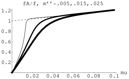
(a) $\,f_{A}/f$

(b) $\,m_{\pi^{\pm}}^{2}$

Figure 5: Examples of quark-mass dependence when using a critical mass with an error of $O(a)$ [method (iv) of Fig. 1]: (a) $f_{A}/f$ and (b) $m_{\pi^{\pm}}^{2}$ (in GeV²) versus $\mu$ (in GeV) The parameter-set is described in the text, and corresponds to the first-order transition scenario. $m^{\prime\prime}$ is fixed to $\delta m$, with values $0.005$, $0.015$ and $0.025$ GeV. These are distinguished by the line width, which increases with the magnitude of $\delta m$. The dashed line shows the continuum result.

(a) $\,f_{A}/f$

(b) $\,m_{\pi^{\pm}}^{2}$

Figure 6: As in Fig. 5 except that the sign of $w^{\prime}$ is changed so that one is in the Aoki-phase scenario. In addition, the values of $\delta m$ are chosen to be negative in (b).

In all the plots the dashed lines are the continuum results for the parameters I have chosen, assuming that one is at maximal twist. The solid lines illustrate the dependence on the twisted mass $\mu$ for three choices of the untwisted mass $\delta m$. I use $\delta m=25$, $15$ and $5\;$MeV, except in Fig. 6(b), where I use $-25$, $-15$ and $-5\;$MeV. These values are chosen to bracket the GSM and Aoki regimes (recall that $a^{2}\Lambda_{\rm QCD}^{3}=7.5\;$MeV for $a^{-1}=2\;$GeV). The largest value of $|\delta m|$ (giving the curves with the thickest lines) is most representative of method (iv), i.e. it has $\delta m\sim a$ for typical choices of $a$. The curves for $|\delta m|=25\;$MeV bend away from the continuum form for $\mu\mathrel{\hbox to0.0pt{\lower 3.0pt\hbox{$\mathchar 536\relax$}\hss}\raise 2.0pt\hbox{$\mathchar 316\relax$}}\delta m$, as expected from eqs. (37) and (38). The NLO corrections are significant, however, as can be seen from the fact that the results are different for first-order and Aoki-phase scenarios. In other words, the results depend on the choice of $w^{\prime}$, which is a NLO parameter in the GSM regime, rather than just on $|\delta m|$ and $\mu$, as predicted by the LO results.

I include the results for $|\delta m|=5\;$MeV to illustrate what happens if one enters into the Aoki regime. These do not correspond to method (iv) as defined above, and the expressions (37) and (38) are not valid when $\mu\approx|\delta m|$. This can be seen clearly from the $\delta m=5\;$MeV curves for the first-order scenario in Fig. 5: they are not smooth, and there is a very large difference between them and those for the Aoki-phase scenario. I choose negative values for $\delta m$ in Fig. 6 so that only the $\delta m=-5\;$MeV result corresponds to running into the Aoki phase—indeed this curve shows what happens when one runs into an end-point of the Aoki phase, while those for $\delta m=-15$ and $-25\;$MeV avoid the phase boundary. The deviations from the continuum result are also larger for negative than for positive $\delta m$ (another indication that the LO expressions are insufficient).

The intermediate choice $|\delta m|=15\;$MeV lies at, or close to, the boundary of the Aoki regime, depending on the value of $a$, and I include it for completeness.

Although the discussion in this section is mainly theoretical, it is interesting to know whether method (iv) has been used in practice, i.e. whether the error in $m_{c}$ is of $O(a)$ or smaller. This is not entirely clear. The traditional method for determining $m_{c}$ has been to extrapolate $m_{\pi}^{2}$ to zero along the Wilson axis with a simple fit function starting from relatively large quark masses. There are two issues that arise in evaluating this “$m_{\pi}=0$” method. First, even if one did a perfect extrapolation, the result would differ by $O(a^{2})$ from an optimal critical mass ShSi ; AB04 . Second, the long extrapolation introduces a systematic error which, while not parametrically of $O(a)$, may be numerically of $O(a)$ in a given simulation. For example, in the case where there is an Aoki phase (as appears to be true for quenched simulations with the Wilson gauge action), the extrapolation might miss the actual end-point by an amount of $O(a)$. If so, one would be using what I am calling method (iv).

The quenched studies of Refs. Biet04 ; Lewis ; Jansen05 ; nobend05 compare the results at maximal twist using the “$m_{\pi}=0$” definition of the critical mass to those obtained with an optimal choice (using methods (i) or (ii), or, in the case of Ref. Biet04 , results from overlap fermions). The results using the former definition are found to bend away from those with an optimal $m_{c}$ for $\mu\mathrel{\hbox to0.0pt{\lower 3.0pt\hbox{$\mathchar 536\relax$}\hss}\raise 2.0pt\hbox{$\mathchar 316\relax$}}a$. In light of the previous discussion, however, it is unclear whether the “$m_{\pi}=0$” definition corresponds to method (iv), and thus one does not know which of the curves in Figs. 5 or 6 best illustrate the expected behavior. For example, in the $\beta=6$ data of Ref. Lewis , the value of $\delta m$ is found to be approximately $0.01(Z_{m}/a)\approx 20\;$MeV. Given that $a\Lambda_{\rm QCD}^{2}\approx 45\;$MeV and $a^{2}\Lambda_{\rm QCD}^{3}\approx 7\;$MeV for this simulation, it is unclear whether $\delta m$ should be treated as of $O(a)$ or $O(a^{2})$. From a practical viewpoint, however, this is not important. One should attempt to fit the results to the NLO tm$\chi$PT forms keeping $\delta m$ as a free parameter.

V.2 Optimal critical mass

I now return to the case of an optimal $m_{c}$. The discussion follows a similar line to that for a non-optimal $m_{c}$, but in this case there are no simple analytic forms to illustrate the summation.

In the analysis of Ref. FMPR , the apparent IR divergences are suppressed because, by construction, the single pion matrix elements of $a\ell_{5}$ are reduced from $\sim a$ to $\sim a\mu,a^{3}$ (and are thus the same size as the matrix element of $a^{3}\ell_{7}$ if $\mu\sim a^{2}$). The dominant terms are of the form $a^{2}(a^{2}/m_{\pi}^{2})^{k}$, with $k\geq 1$, and so are all equally important when $m_{\pi}^{2}\sim a^{2}$, at which point they are all $\sim a^{2}$. These terms apparently preclude one from working in the Aoki regime, for although the errors are parametrically small (proportional to $a^{2}$) they have a complicated and non-uniform dependence on the lattice spacing and quark mass. Furthermore, the Symanzik expansion is apparently breaking down.

The tm$\chi$PT analysis shows, however, that, as above, the IR divergences indicate expansion about the wrong vacuum and can be summed by implementing a non-perturbative shift to the correct vacuum. As noted in Ref. FMPR , the leading IR divergences result from multiple insertions of $\ell_{6}$, with only one creation of a neutral pion by the suppressed vertex $\ell_{5,7}$. Correspondingly, in the tm$\chi$PT analysis the change of vacuum is that caused by the $a^{2}$ coefficient $w^{\prime}$. This is exactly the analysis of the phase structure in the Aoki regime carried out previously in Refs. Mun04 ; Scor04 ; AB04 ; ShWu1 , and extended here to NLO. The results for $f_{A}/f$ and $m_{\pi}^{2}$ are exemplified by the $|\delta m|=5\;$MeV curves in Figs. 5 and 6.

The conclusions I draw are as follows. First, there is no obstacle, in general, to simulating in the Aoki regime. The tm$\chi$PT analysis provides functional forms that allow one to predict and fit the behavior of physical quantities in this regime. There is, in other words, no breakdown of theoretical understanding in this region, and in particular no breakdown of the Symanzik expansion, in the sense that once one includes the leading effects of $\ell_{6}$ non-perturbatively, the subleading contributions from these operators, and the contributions of higher order operators (including now $\ell_{5}$), are systematically suppressed by the expected powers of $a\Lambda_{\rm QCD}$. In fact, if one works at maximal twist, defined using any of methods (i-iii) (with the caveat that one must stay above the end-point in the first-order scenario), then the contributions of $\ell_{6}$ remain perturbative also, along with their manifest powers of $a$. This is because, when using any of these methods, the condensate points in direction of maximal twist up to small corrections, $\omega_{m}=\pi/2+O(a)$.

Second, although the apparent IR divergences are summed up by tm$\chi$PT, their “residue” is a complicated dependence of physical quantities on $a$ and $\mu$. Third, and most important from a practical point of view, if one works at maximal twist using any of methods (i-iii), then the continuum extrapolations are not complicated. Indeed, as already noted in the previous section, there are no $a^{2}$ (or $a^{3}$) corrections to the charged pion masses in this case. Thus in the Aoki-phase scenario, there is no obstacle to working all the way down to $\mu=0$, although in the first-order scenario one must stop at $|\mu|\mathrel{\hbox to0.0pt{\lower 3.0pt\hbox{$\mathchar 536\relax$}\hss}\raise 2.0pt\hbox{$\mathchar 318\relax$}}2w^{\prime}$. Nevertheless, the overall point is that one does not need to impose the constraint $m_{q}\sim\mu>a^{2}$ AB04 ; ShWu2 .

There is an exception to the claim that tm$\chi$PT controls the IR divergences. This is in the vicinity of the end-points of the phase-boundary. Here, as discussed in the previous section, the power counting of tm$\chi$PT breaks down, and higher order terms, including loops, are needed to determine the vacuum. Thus, in the first order scenario, one should work at maximal twist only until one is a distance $\delta\mu\sim a^{3}$ away from the transition.

V.3 Subleading IR divergences

The analysis of Ref. FMPR points out that, in addition to the leading order IR divergences, there are subleading IR divergent contributions. Although the former have been understood and summed using tm$\chi$PT, what of the latter? I have not done a complete analysis of this question, but I think the above analysis of the leading divergences makes the following conjecture reasonable: the subleading IR divergences are removed by a small shift in the vacuum, perturbatively calculable in tm$\chi$PT (except near the end-points). This incorporates the NLO and higher order effects of $\ell_{5}$ and $\ell_{6}$, as well as the contributions of higher order operators. In other words, I conjecture that there is no breakdown of the Symanzik expansion, in the sense described above, as long as one uses tm$\chi$PT to include the dominant terms ($\ell_{5}$ in the GSM regime and $\ell_{6}$ in the Aoki regime) non-perturbatively. Progressively higher order terms ($\ell_{7}$, $\ell_{8}$, etc.) will then have progressively smaller effects, each subsequent order suppressed by $a\Lambda_{\rm QCD}$.

This brings me to the logical relation between the approach of Ref. FMPR and tm$\chi$PT. I want to reiterate that the starting point of tm$\chi$PT is the Symanzik expansion, but that tm$\chi$PT goes beyond by including our non-perturbative understanding of spontaneous chiral symmetry breaking. Thus it is based on a tower of two local effective theories: the first describing the long-distance physics of lattice QCD, and the second describing the long-distance behavior of the first. The theoretical status of the second effective theory, i.e. chiral perturbation theory, is, perhaps, less solid than the first, since one cannot do a perturbative analysis following Symanzik Symanzik as chiral symmetry breaking is a non-perturbative phenomenon. Nevertheless, the theoretical basis for tm$\chi$PT, which is identical to that for continuum $\chi$PT, is strong Weinberg ; Leutwyler . The main shortcoming of tm$\chi$PT, I believe, is not its theoretical foundation, but rather the practical need to truncate the expansion at NLO or, perhaps, NNLO, and the related issue of how well the expansion converges for present quark masses and lattice spacings. In this regard, the present analysis and the conjecture made above are important, because they imply that there is no non-uniformity in a joint expansion in $m_{q}$ and $a$. The absence of IR divergent terms implies that one makes only small errors by truncating the Symanzik expansion at, say, $\ell_{7}$ (as is done in the previous section).

VI Conclusions

Studies of tmLQCD are still at a relatively early stage, and it is important to fully understand the practical and theoretical issues that are involved. Key issues are the determination of the critical mass and the size, and chiral behavior, of the remaining discretization errors. Particularly important discretization errors are those giving rise to parity and flavor breaking, for unless these are small in practice they will likely lead to complications in extracting phenomenologically important hadronic quantities.

Here I have focused on the theoretical issues, showing how by applying chiral perturbation theory to Symanzik’s effective Lagrangian one can systematically study the properties of discretization errors. The aim here is to understand the errors so that they can be removed, or reduced, in a controlled way. For example, if one wants to work at maximal twist, where the errors of $O(a)$ are automatically removed, then it is useful to know what happens when the choice of critical mass has errors of a given size. The forms given in Ref. ShWu2 and generalized here provide such information to NLO in the joint chiral-continuum expansion. In particular, I have extended previous results in the Aoki regime to NLO, allowing consistent NLO fits for all quark masses.

On a practical level, there is general agreement in the literature on how to proceed: one should use one of the “optimal” non-perturbative definitions of maximal twist [methods (i), (ii) or (iii)]. Here I have clarified the relation between the different definitions, both in the GSM and Aoki regimes.

There is however, disagreement on the interpretation of what happens to discretization errors as one approaches the chiral limit. With non-optimal choices of the critical mass (including the “$m_{\pi}=0$” definition irrespective of the accuracy of the extrapolation) the results for a number of physical quantities exhibit a “bending” effect, in which the results diverge away from the expected chiral behavior for $m_{q}\mathrel{\hbox to0.0pt{\lower 3.0pt\hbox{$\mathchar 536\relax$}\hss}\raise 2.0pt\hbox{$\mathchar 316\relax$}}a$. These can be understood qualitatively in tm$\chi$PT as a result of working at a non-maximal twist angle, with the divergence from $\pi/2$ increasing toward the chiral limit ShWu2 . Examples of the expected forms are given in Figs. 5 and 6. A seemingly different interpretation has been given in Ref. FMPR , in which the bending is due to discretization errors which are proportional to inverse powers of the quark mass, and which, for $m_{q}\sim a$, arise from contributions proportional to all powers of $a$. I have shown, however, that the interpretations are consistent: the apparently IR divergent errors of Ref. FMPR are simply an expansion of the convergent expressions of tm$\chi$PT, and indicate the need to do a non-perturbative shift in the vacuum.

A similar discussion applies to the discretization errors that arise when one works with an optimal choice of maximal twist. The IR divergent errors analyzed in Ref. FMPR are summed up by tm$\chi$PT applied in the Aoki regime. One consequence is that there is no barrier to working at maximal twist in this regime, i.e. with $m_{q}\sim a^{2}$, as long as one uses the optimal choice of maximal twist determined in this regime (rather than by extrapolation from larger masses) and as long as one does not work all the way down to the second-order end-points if one is in the scenario with a first-order transition.

It is suggested in Ref. FMPR that the apparent IR divergences signal a breakdown of the Symanzik expansion at small quark masses ($m_{q}\sim a^{2}$ for an optimal choice of maximal twist). I have argued that this is not the case, although the situation is somewhat subtle. The apparent IR divergences are an indication that, in general, the leading terms in the Symanzik expansion (those proportional to $a$ and $a^{2}$) must be treated non-perturbatively, and this is what is accomplished by tm$\chi$PT. This might be interpreted as a breakdown in the simple expansion in powers of lattice spacing, since insertions of any number of factors of $\ell_{5}$ and $\ell_{6}$ are required. On the other hand, one can treat subsequent terms, $\ell_{7}$, $\ell_{8}$, etc., as small corrections, so in this sense the expansion remains intact. In fact, at maximal twist, defined optimally, the contributions of $\ell_{5}$ and $\ell_{6}$ can also be treated perturbatively, so the Symanzik expansion remains valid in the usual sense that all powers of $a$ are manifest. It is for this reason that automatic improvement at maximal twist remains valid into the Aoki region (and all the way down to $m_{q}=0$ in the Aoki-phase scenario AB04 ; ShWu2 ). This result should simplify numerical applications of tmLQCD.

After this paper was completed, Ref. AB05 appeared, containing results overlapping those in secs. II, III and IV, as well as detailed fits of numerical results to tm$\chi$PT expressions.

References

-
(1)
R. Frezzotti, P. A. Grassi, S. Sint and P. Weisz,
Nucl. Phys. Proc. Suppl. 83, 941 (2000)
[arXiv:hep-lat/9909003];
and
JHEP 0108, 058 (2001)
[arXiv:hep-lat/0101001];
R. Frezzotti, S. Sint and P. Weisz [ALPHA collaboration], JHEP 0107, 048 (2001) [arXiv:hep-lat/0104014]. - (2) R. Frezzotti and G. C. Rossi, JHEP 0408, 007 (2004) [arXiv:hep-lat/0306014].
- (3) R. Frezzotti and G. C. Rossi, JHEP 0410, 070 (2004) [arXiv:hep-lat/0407002].
- (4) R. Frezzotti and G. Rossi, arXiv:hep-lat/0507030.
- (5) R. Frezzotti, Nucl. Phys. Proc. Suppl. 140, 134 (2005) [arXiv:hep-lat/0409138].
- (6) A. Shindler, plenary talk at Lattice 2005, to appear in the proceedings.
- (7) R. Frezzotti and G. C. Rossi, Nucl. Phys. Proc. Suppl. 128, 193 (2004) [arXiv:hep-lat/0311008].
- (8) S. R. Sharpe and R. L. Singleton, Phys. Rev. D 58, 074501 (1998) [arXiv:hep-lat/9804028].
- (9) G. Rupak and N. Shoresh, Phys. Rev. D 66, 054503 (2002) [arXiv:hep-lat/0201019].
- (10) O. Bär, G. Rupak and N. Shoresh, Phys. Rev. D 70, 034508 (2004) [arXiv:hep-lat/0306021].
- (11) G. Münster and C. Schmidt, Europhys. Lett. 66, 652 (2004) [arXiv:hep-lat/0311032].
- (12) S. Aoki and O. Bär, Phys. Rev. D 70, 116011 (2004) [arXiv:hep-lat/0409006].
- (13) S. R. Sharpe and J. M. S. Wu, Phys. Rev. D 71, 074501 (2005) [arXiv:hep-lat/0411021].
- (14) G. Munster, JHEP 0409, 035 (2004) [arXiv:hep-lat/0407006].
- (15) L. Scorzato, Eur. Phys. J. C 37, 445 (2004). [arXiv:hep-lat/0407023].
- (16) S. R. Sharpe and J. M. S. Wu, Phys. Rev. D 70, 094029 (2004) [arXiv:hep-lat/0407025].
- (17) R. Frezzotti, G. Martinelli, M. Papinutto and G. C. Rossi, arXiv:hep-lat/0503034.
- (18) K. Symanzik, Nucl. Phys. B226, 187 (1983); B226, 205 (1983).
- (19) S. Weinberg, PhysicaA 96, 327 (1979).
- (20) H. Leutwyler, Annals Phys. 235, 165 (1994) [arXiv:hep-ph/9311274].
- (21) J. Gasser and H. Leutwyler, Annals Phys. 158, 142 (1984); Nucl. Phys. B 250, 465 (1985).
- (22) F. Farchioni et al., Eur. Phys. J. C 42, 73 (2005) [arXiv:hep-lat/0410031].
- (23) A. M. Abdel-Rehim, R. Lewis and R. M. Woloshyn, Phys. Rev. D 71, 094505 (2005) [arXiv:hep-lat/0503007].
- (24) K. Jansen, M. Papinutto, A. Shindler, C. Urbach and I. Wetzorke [XLF Collaboration], Phys. Lett. B 619, 184 (2005) [arXiv:hep-lat/0503031].
- (25) S. Aoki, Phys. Rev. D 30, 2653 (1984); Phys. Rev. Lett. 57, 3136 (1986); Prog. Theor. Phys. 122, 179 (1996).
- (26) S. Aoki, Phys. Rev. D 68, 054508 (2003) [arXiv:hep-lat/0306027].
- (27) K. Jansen, M. Papinutto, A. Shindler, C. Urbach and I. Wetzorke [XLF Collaboration], arXiv:hep-lat/0507010.
- (28) A. Walker-Loud and J. M. S. Wu, Phys. Rev. D 72, 014506 (2005) [arXiv:hep-lat/0504001].
- (29) W. Bietenholz et al. [XLF Collaboration], JHEP 0412, 044 (2004) [arXiv:hep-lat/0411001].
- (30) S. Aoki and O. Bär, arXiv:hep-lat/0509002.