$B^{0}-\bar{B}^{0}$ mixing in the static approximation from the Schrödinger Functional and twisted mass QCD

Abstract:

We discuss the renormalisation properties of parity-odd $\Delta B=2$ operators with the heavy quark treated in the static approximation. Via twisted mass QCD (tmQCD), these operators provide the matrix elements relevant for the $B^{0}-\bar{B}^{0}$ mixing amplitude. The layout of a non-perturbative renormalisation programme for the operator basis, using Schrödinger Functional techniques, is described. Finally, we report our results for a one-loop perturbative study of various renormalisation schemes with Wilson-type lattice regularisations, which allows, in particular, to compute the NLO anomalous dimensions of the operators in the SF schemes of interest.

PoS(LAT2005)214

1 Introduction

The oscillations of the system $B^{0}-\bar{B}^{0}$ are one of the crucial topics in particle physics. Their understanding represents a challenging bridge towards the numerical determination of the Cabibbo-Kobayashi-Maskawa (CKM) matrix and a severe test of the Standard Model. The transition amplitude responsible for the mixing,

$$\langle\bar{B}^{0}|{\cal O}_{\rm VV+AA}|B^{0}\rangle=\frac{8}{3}f_{B}^{2}m_{B}^{2}B_{B},$$ (1)

is mediated by the four-quark operator ${\cal O}_{\rm VV+AA}=(\bar{b}\gamma_{\mu}d)(\bar{b}\gamma_{\mu}d)+(\bar{b}\gamma_{\mu}\gamma_{5}d)(\bar{b}\gamma_{\mu}\gamma_{5}d)$. It has been shown that the renormalisation of such operators is non-trivial in Wilson-like regularisations, resulting in a mixing with other four-quark operators [1]. Here we propose a strategy to compute the matrix element, based on the static approximation of the heavy quark plus the adoption of a tmQCD regularisation for the light one. It will be proved that, following these assumptions, the mixing under renormalisation is eliminated. Of course, the potential results of the proposed approach constitute an intermediate step to the physical solution, as they must be considered in view of the calculation of heavy quark subleading corrections and/or interpolations to relativistic calculations performed at accessible heavy quark masses [2].

2 Operator mapping in tmQCD

In order to implement our strategy, we start by fixing the notation. The $b$ quark is replaced by an infinitely massive quark, described by a pair of static fields $(\psi_{h},\psi_{\bar{h}})$ propagating forward and backward in time, whose dynamics is governed by the Eichten-Hill action [3] (or one of its ALPHA variants [4]),

$$S^{\rm stat}[\psi_{h},\psi_{\bar{h}}]=a^{4}\sum_{x}\left[\bar{\psi}_{h}(x)\nabla_{0}^{*}\psi_{h}(x)-\bar{\psi}_{\bar{h}}(x)\nabla_{0}\psi_{\bar{h}}(x)\right].$$ (2)

On the light quark side, the degrees of freedom are represented by an isospin doublet $\psi_{\ell}^{T}=(u,d)$, made of an up and a down quark, and described according to the tmQCD action,

$$S^{\rm tmQCD}=a^{4}\sum_{x}\ \left\{\psi_{\ell}(x)\left[{\kern 2.5pt/\kern-6.99997ptD}+m_{\ell}+i\mu_{\ell}\tau^{3}\gamma_{5}\right]\psi_{\ell}(x)\right\}.$$ (3)

The equivalence of this regularisation to ordinary QCD, established in [6], is based on axial transformations of the quark fields (plus the corresponding spurionic transformations of the mass parameters $m_{\ell}$ and $\mu_{\ell}$), which induce a rotation of composite operators between the two theories. In particular, for the operator under study one has

$$\left({\cal O}_{\rm VV+AA}\right)_{\rm R}^{\rm QCD}=\cos(\alpha)\left({\cal O}_{\rm VV+AA}\right)_{\rm R}^{\rm tmQCD,\alpha}-i\sin(\alpha)\left({\cal O}_{\rm VA+AV}\right)_{\rm R}^{\rm tmQCD,\alpha}\ ,$$ (4)

where the terms have to be interpreted as operator insertions in renormalised Green functions in the continuum limit, and a mass-independent renormalisation scheme is assumed. Following the notation of [6], the twist angle $\alpha$ depends upon the renormalised mass parameters through the relation $\tan(\alpha)=\mu_{\ell;{\rm R}}/m_{\ell;{\rm R}}$, and (4) is an identity holding at each value of $\alpha$. In particular, at $\alpha=\pi/2$, which is known as the fully twisted case, (4) simplifies to

$$\left({\cal O}_{\rm VV+AA}\right)_{\rm R}^{\rm QCD}=-i\left({\cal O}_{\rm VA+AV}\right)_{\rm R}^{\rm tmQCD,\pi/2}\ .$$ (5)

In this way, ${\cal O}_{\rm VV+AA}$ in standard QCD is mapped onto its counterpart ${\cal O}_{VA+AV}$ in tmQCD. Using the mass independence of the renormalisation scheme, we will show in the next section that ${\cal O}_{\rm VA+AV}$ renormalises multiplicatively in the static approximation, which represents the main advantage of using the above mapping. In this sense, the proposed approach represents an extension to the static case of the tmQCD framework used to determine the $B_{K}$ parameter [7, 8].

3 Renormalisation pattern

We now concentrate on the renormalisation properties of heavy-light four-quark operators, with the aim of proving that ${\cal O}_{\rm VA+AV}$ renormalises multiplicatively. Unfortunately, for brevity’s sake, we skip algebraic details [10]. We start by considering generic four-quark operators

$$O^{\pm}_{\Gamma_{1}\Gamma_{2}}=\dfrac{1}{2}\left[(\bar{\psi}_{h}\Gamma_{1}\psi_{1})(\bar{\psi}_{\bar{h}}\Gamma_{2}\psi_{2})\pm(\bar{\psi}_{h}\Gamma_{1}\psi_{2})(\bar{\psi}_{\bar{h}}\Gamma_{2}\psi_{1})\right],$$ (6)

where $\Gamma_{1,2}$ represent Dirac matrices. In principle, operators corresponding to different Dirac structures could mix among them under renormalisation, thus giving rise to a matrix renormalisation pattern; consequently a complete basis of such operators must be considered, such as

$${\rm parity-even:~{}~{}}Q_{1}^{\pm} =O^{\pm}_{\rm VV+AA}\ ,\qquad{\rm parity-odd:~{}~{}} {{\cal Q}}_{1}^{\pm} =O^{\pm}_{\rm VA+AV}\ ,$$

$$Q_{2}^{\pm} =O^{\pm}_{\rm SS+PP}\ , {{\cal Q}}_{2}^{\pm} =O^{\pm}_{\rm SP+PS}\ ,$$

$$Q_{3}^{\pm} =O^{\pm}_{\rm VV-AA}\ , {{\cal Q}}_{3}^{\pm} =O^{\pm}_{\rm VA-AV}\ ,$$

$$Q_{4}^{\pm} =O^{\pm}_{\rm SS-PP}\ , {{\cal Q}}_{4}^{\pm} =O^{\pm}_{\rm SP-PS}\ .$$ (7)

The renormalisation matrix ${\mathds{Z}}$, whose size is in principle $8\times 8$ (mixing between $+$ and $-$ operators is trivially excluded), can be constrained through symmetry arguments. Given a symmetry of the theory, and the matrix $\Phi$ that implements a symmetry transformation at the level of the operator basis, it is sufficient to require that ${\mathds{Z}}$ is invariant under a $\Phi$-rotation [9], i.e.

$${\mathds{Z}}=\Phi{\mathds{Z}}\Phi^{-1}\ .$$ (8)

The symmetries we use are:

• Parity. It prevents the mixing among operators with opposite parity. After implementing it, the renormalisation matrix ${\mathds{Z}}$ is reduced to a block-diagonal form, where two $4\times 4$ diagonal blocks describe the mixing of the parity-even and parity-odd operators among themselves.

• Chiral simmetry. It is used à la [1]: were chirality respected by the regulator, there would be no chance of mixing among different chirality sectors. The mixing due to the Wilson chirality breaking in the parity-odd sector can be represented according to the form

  $$\left(\begin{array}[]{c}{\cal Q}_{1}^{\pm}\\ {\cal Q}_{2}^{\pm}\\ {\cal Q}_{3}^{\pm}\\ {\cal Q}_{4}^{\pm}\end{array}\right)_{\rm R}=\left(\begin{array}[]{cccc}{\cal Z}_{11}^{\pm}&{\cal Z}_{12}^{\pm}&0&0\\ {\cal Z}_{21}^{\pm}&{\cal Z}_{22}^{\pm}&0&0\\ 0&0&{\cal Z}_{33}^{\pm}&{\cal Z}_{34}^{\pm}\\ 0&0&{\cal Z}_{43}^{\pm}&{\cal Z}_{44}^{\pm}\end{array}\right){\left[\mathds{1}+\left(\begin{array}[]{cccc}0&0&\Delta_{13}^{\pm}&\Delta_{14}^{\pm}\\ 0&0&\Delta_{23}^{\pm}&\Delta_{24}^{\pm}\\ \Delta_{31}^{\pm}&\Delta_{32}^{\pm}&0&0\\ \Delta_{41}^{\pm}&\Delta_{42}^{\pm}&0&0\end{array}\right)\right]}\left(\begin{array}[]{c}{\cal Q}_{1}^{\pm}\\ {\cal Q}_{2}^{\pm}\\ {\cal Q}_{3}^{\pm}\\ {\cal Q}_{4}^{\pm}\end{array}\right),$$ (25)

  where the coefficients ${\cal Z}_{ij}$ are scale dependent, while the $\Delta_{ij}$’s are not.

• Heavy quark spin symmetry and H(3) spatial rotations. We then consider two finite spin rotations of the heavy fields, plus two lattice spatial rotations of both heavy and light fields

  heavy quark spin rotations: $$\bar{\psi}_{h}\to\bar{\psi}_{h}\gamma_{2}\gamma_{3},\quad\bar{\psi}_{\bar{h}}\to\bar{\psi}_{\bar{h}}\gamma_{2}\gamma_{3},$$

  $$\bar{\psi}_{h}\to\bar{\psi}_{h}\gamma_{3}\gamma_{1},\quad\bar{\psi}_{\bar{h}}\to\bar{\psi}_{\bar{h}}\gamma_{3}\gamma_{1},$$

  lattice spatial rotations: $${\cal R}(\ \hat{1}\to\hat{2}\ )\ \mbox{rotates the $\hat{1}$ axis onto the $\hat{2}$ axis},$$

  $${\cal R}(\ \hat{1}\to\hat{3}\ )\ \mbox{rotates the $\hat{1}$ axis onto the $\hat{3}$ axis.}$$ (26)

  After a change of basis and some tedious algebra, the parity violating block reduces to

  $$\left(\begin{array}[]{c}\hskip-4.26773pt{\cal Q}_{1}^{\pm}\\ \hskip-4.26773pt{\cal Q}_{1}^{\pm}+4\hat{\cal Q}_{2}^{\pm}\\ \hskip-4.26773pt{\cal Q}_{3}^{\pm}+2\hat{\cal Q}_{4}^{\pm}\\ \hskip-4.26773pt{\cal Q}_{3}^{\pm}-2\hat{\cal Q}_{4}^{\pm}\end{array}\hskip-4.26773pt\right)_{\rm R}=\left(\begin{array}[]{cccc}\hskip-4.26773pt{\cal Z}_{1}^{\pm}&\hskip-4.26773pt0&\hskip-4.26773pt0&\hskip-4.26773pt0\\ \hskip-4.26773pt0&\hskip-4.26773pt{\cal Z}_{2}^{\pm}&\hskip-4.26773pt0&\hskip-4.26773pt0\\ \hskip-4.26773pt0&\hskip-4.26773pt0&\hskip-4.26773pt{\cal Z}_{3}^{\pm}&\hskip-4.26773pt0\\ \hskip-4.26773pt0&\hskip-4.26773pt0&\hskip-4.26773pt0&\hskip-4.26773pt{\cal Z}_{4}^{\pm}\end{array}\hskip-4.26773pt\right){\left[\mathds{1}+\left(\begin{array}[]{cccc}\hskip-4.26773pt0&0&\Delta_{1}^{\pm}&0\\ \hskip-4.26773pt0&0&0&\Delta_{2}^{\pm}\\ \hskip-4.26773pt\Delta_{3}^{\pm}&0&0&0\\ \hskip-4.26773pt0&\Delta_{4}^{\pm}&0&0\end{array}\hskip-4.26773pt\right)\right]}\left(\begin{array}[]{c}\hskip-4.26773pt{\cal Q}_{1}^{\pm}\\ \hskip-4.26773pt{\cal Q}_{1}^{\pm}+4{\cal Q}_{2}^{\pm}\\ \hskip-4.26773pt{\cal Q}_{3}^{\pm}+2{\cal Q}_{4}^{\pm}\\ \hskip-4.26773pt{\cal Q}_{3}^{\pm}-2{\cal Q}_{4}^{\pm}\end{array}\hskip-4.26773pt\right).$$ (43)

• Time reversal. We finally consider a time reversal transformation of the quark fields:

  $$\psi_{h}(x)\to\gamma_{0}\gamma_{5}\psi_{\bar{h}}(x^{\tau}),\quad\psi_{\bar{h}}(x)\to\gamma_{0}\gamma_{5}\psi_{h}(x^{\tau}),\quad\psi_{k}(x)\to\gamma_{0}\gamma_{5}\psi_{k}(x^{\tau}),\quad k=1,2.$$ (44)

  It further constrains the parity-odd block by forcing the residual $\Delta_{i}$ coefficients in (3.6) to vanish. Purely multiplicative renormalisation of ${\cal Q}_{\rm VA+AV}^{\pm}$ follows therefrom.

4 Renormalisation in Schrödinger Functional schemes

We use the Schrödinger Functional (SF) to define a family of finite volume renormalisation schemes, in view of a non-perturbative study of the running of the ${\cal O}_{VA+AV}$ operator. Our approach closely follows here refs. [7], to which the reader is referred for unexplained notation. We first introduce bilinear boundary sources at $x_{0}=0,T$ (being $T$ the time extension of the SF),

$${\cal S}_{s_{1}s_{2}}[\Gamma] =a^{6}\sum_{\mathbf{x},\mathbf{y}}\bar{\zeta}_{s_{1}}(\mathbf{x})\Gamma\zeta_{s_{2}}(\mathbf{y})\ ,\qquad{\cal S}^{\prime}_{s_{1}s_{2}}[\Gamma]=a^{6}\sum_{\mathbf{x},\mathbf{y}}\bar{\zeta}^{\prime}_{s_{1}}(\mathbf{x})\Gamma\zeta^{\prime}_{s_{2}}(\mathbf{y})\ ,$$ (45)

where $\Gamma$ is a Dirac matrix and the flavour indices $s_{1,2}$ can assume either relativistic or static values. Then, we define a set of SF correlators in order to probe the operators ${\cal Q}^{\pm}_{1}$,

$$F_{1}^{\pm}(x_{0})=\frac{a^{3}}{L^{3}}\sum_{\bf x}\langle{\cal S}^{\prime}_{3\bar{h}}[\Gamma_{3}]{{\cal Q}}_{1}^{\pm}(x){\cal S}_{1h}[\Gamma_{1}]{\cal S}_{23}[\Gamma_{2}]\rangle\ ,$$

$$f_{1}^{s_{1}s_{2}}=-\frac{1}{L^{6}}\langle{\cal S}^{\prime}_{s_{1}s_{2}}[\gamma_{5}]{\cal S}_{s_{2}s_{1}}[\gamma_{5}]\rangle\ ,\qquad k_{1}^{s_{1}s_{2}}=-\frac{1}{3L^{6}}\sum_{k=1}^{3}\langle{\cal S}^{\prime}_{s_{1}s_{2}}[\gamma_{k}]{\cal S}_{s_{2}s_{1}}[\gamma_{k}]\rangle\ .$$ (46)

The triple $[\Gamma_{1},\Gamma_{2},\Gamma_{3}]$ has to be chosen such that $F_{1}^{\pm}$ is non-zero. The boundary correlators $f_{1}$ and $k_{1}$, which can have either light-light or heavy-light flavour structure, are needed in order to cancel the renormalisation of the boundary sources in $F_{1}^{\pm}$. In practice, we consider ratios of the form

$$h_{1}^{\pm}(x_{0})=\frac{F_{1}^{\pm}(x_{0})}{f_{1}^{hl}\ [f_{1}^{ll}]^{\alpha}\ [k_{1}^{ll}]^{1/2-\alpha}\ }$$ (47)

and then impose in the chiral limit the renormalisation condition

$${\cal Z}_{1}^{\pm}h_{1}^{\pm}(T/2)=h_{1}^{\pm}(T/2)|_{g_{0}=0}.$$ (48)

Of course, the renormalisation factor ${\cal Z}_{1}^{\pm}$ depends upon all calculational details, e.g. the light quark action (Wilson with(out) a clover term), the static action (Eichten-Hill, or its ALPHA variants), the choice of the Dirac structures $[\Gamma_{1},\Gamma_{2},\Gamma_{3}]$, the value of the $\theta$-angle of the SF and the value of the parameter $\alpha$ introduced in (47). This richness of degrees of freedom can be exploited in order to identify some optimal renormalisation schemes, according to the general requirements of maximisation of the nonperturbative signal/noise ratio, slowing down of the operator running and minimisation of lattice artefacts.

5 NLO anomalous dimension of ${\cal Q}_{1}^{+}$ from perturbative matching at one-loop order

In order to gain information about the running and its lattice artefacts, we have performed a one-loop perturbative calculation of the renormalisation factor ${\cal Z}^{+}_{1}$ in some of the SF schemes discussed above. Such a calculation allows us to determine the NLO anomalous dimension of ${\cal Q}_{1}^{+}$ via a perturbative matching to some reference scheme in which the NLO anomalous dimension is already known. The matching procedure has been illustrated and applied several times in the literature [11, 7, 12], and it will not be reviewed here. The reference scheme was chosen to be DRED, where the NLO anomalous dimension of ${\cal Q}_{1}^{+}$ and its perturbative matching to the so-called lat-scheme have been computed in [13]. The perturbative expansion of ${\cal Z}_{1}^{+}$ reads

$${\cal Z}_{1}^{+}(g_{0}^{2},a/L)=1+\sum_{k=1}^{\infty}g_{0}^{2k}{\cal Z}_{1}^{+(k)}=1+g_{0}^{2}\left[r_{0}^{+}+\gamma_{0}^{+}\ln\left(\frac{a}{L}\right)+O\left(\frac{a}{L}\right)\right]+O(g_{0}^{4})$$ (49)

where $\gamma_{0}^{+}=-1/(2\pi^{2})$ is the universal anomalous dimension of the operator ${\cal Q}_{1}^{+}$, and $r_{0}^{+}$ is the one-loop scheme-dependent finite part, peculiar to the SF and the defining choices listed at the end of the previous section. The running of the operator is described by the step scaling function (ssf),

$$\sigma_{1}^{+}(u)=\lim_{a\to 0}\frac{{\cal Z}_{1}^{+}(g_{0},a/2L)}{{\cal Z}_{1}^{+}(g_{0},a/L)}\biggr{|}_{\bar{g}^{2}(L)=u}=1+\sum_{k=1}^{\infty}g_{0}^{2k}\sigma_{1}^{+(k)}$$ (50)

As an example of the running, the ssf of ${\cal Q}_{1}^{+}$ at NLO and $N_{\rm f}=0$ is reported as a function of the renormalised coupling on the left side of Figure 1. The plot refers to the choice $[\Gamma_{1},\Gamma_{2},\Gamma_{3}]=[\gamma_{5},\gamma_{5},\gamma_{5}]$. The straight line represents the universal LO running, and the bands describe the dependence of the NLO anomalous dimension upon the choice of $\alpha$, when the latter ranges in the interval $[0,1/2]$. On the right side of Figure 1 we report a comparison of the lattice artefacts $\delta^{+}_{1}(a/L)$ on the ssf, defined as in [11], between the static-light case and the light-light one (data from [7]). The comparison refers to the schemes where $[\Gamma_{1},\Gamma_{2},\Gamma_{3}]=[\gamma_{5},\gamma_{5},\gamma_{5}]$, $\theta=0.5$ and $\alpha=0$. The light quarks are discretised according to the unimproved (W) or the $c_{\rm sw}$-improved (SW) Wilson action, while the static quarks are discretised according to the Eichten-Hill (EH) action. Although the static-light schemes cannot be directly compared to the relativistic ones (where the normalisation of the four-quark correlator is always performed using only the relativistic correlators), the plot shows that the introduction of static quarks does not imply a significant increment of the lattice artefacts in perturbation theory.

6 Acknowledgments

We thank D. Bećirević, M. Della Morte, R. Sommer and especially J. Reyes for useful discussions. F.P. acknowledges the Conference organisers and the Humboldt-Foundation for financial support.

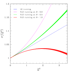
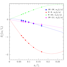
Figure 1: On the left side the step scaling function of ${\cal Q}_{1}^{+}$ at NLO and $N_{\rm f}=0$ is reported vs. the renormalised coupling in the SF scheme. On the right side we compare the lattice artefacts of the step scaling function between the full relativistic case and the static-light case. Both plots are preliminary.

References

• [1] A. Donini et al., Eur. Phys. J. C 10 (1999) 121 [arXiv:hep-lat/9902030].
• [2] D. Bećirević et al. JHEP 0204 (2002) 025 [arXiv:hep-lat/0110091], G. M. de Divitiis et al., Nucl. Phys. B 672, 372 (2003) [arXiv:hep-lat/0307005], J. Rolf et al., Nucl. Phys. Proc. Suppl.  129 (2004) 322 [arXiv:hep-lat/0309072], J. Heitger and R. Sommer, JHEP 0402 (2004) 022 [arXiv:hep-lat/0310035].
• [3] E. Eichten and B. Hill, Phys. Lett. B 234 (1990) 511.
• [4] M. Della Morte, A. Shindler and R. Sommer, JHEP 0508 (2005) 051 [arXiv:hep-lat/0506008].
• [5] M. Della Morte, Nucl. Phys. Proc. Suppl.  140 (2005) 458 [arXiv:hep-lat/0409012].
• [6] R. Frezzotti et al., JHEP 0108 (2001) 058 [arXiv:hep-lat/0101001].
• [7] F. Palombi, C. Pena and S. Sint, [arXiv:hep-lat/0505003]; M. Guagnelli et al., [arXiv:hep-lat/0505002].
• [8] P. Dimopoulos et al., Nucl. Phys. Proc. Suppl.  140 (2005) 362 [arXiv:hep-lat/0409026].
• [9] D. Bećirević and J. Reyes, Nucl. Phys. Proc. Suppl.  129 (2004) 435 [arXiv:hep-lat/0309131].
• [10] F. Palombi, M. Papinutto, C. Pena and H. Wittig, in preparation.
• [11] S. Sint and P. Weisz, Nucl. Phys. B 545 (1999) 529 [arXiv:hep-lat/9808013].
• [12] M. Guagnelli et al., Nucl. Phys. B 664 (2003) 276 [arXiv:hep-lat/0303012].
• [13] V. Giménez and J. Reyes, Nucl. Phys. B 545 (1999) 576 [arXiv:hep-lat/9806023]; J. Reyes, Ph. D. Thesis (in Spanish), Universidad de Valencia, May 2001.