Non-perturbative Power Corrections to Ghost and Gluon Propagators

Abstract

We study the dominant non-perturbative power corrections to the ghost and gluon propagators in Landau gauge pure Yang-Mills theory using OPE and lattice simulations. The leading order Wilson coefficients are proven to be the same for both propagators. The ratio of the ghost and gluon propagators is thus free from this dominant power correction. Indeed, a purely perturbative fit of this ratio gives smaller value ($\simeq 270$MeV) of $\Lambda_{\overline{\text{MS}}}$ than the one obtained from the propagators separately($\simeq 320$MeV). This argues in favour of significant non-perturbative $\sim 1/q^{2}$ power corrections in the ghost and gluon propagators. We check the self-consistency of the method.

1 Introduction

A non-zero value of different QCD condensates leads to non-perturbative power corrections to propagators. The one being intensively studied during last years is the $A^{2}$-condensate in Landau gauge [1, 2, 3, 4, 5, 6] (extended to a gauge-invariant non-local operator, [7]), that is responsible for $\sim 1/q^{2}$ corrections to the gluonic propagator compared to perturbation theory. In this paper we investigate the rôle of such corrections in the ghost propagator, and present a method that allows to test numerically that power corrections of $\sim 1/q^{2}$ type really exist using only ghost and gluon lattice propagators, and ordinary perturbation theory.

The study of the asymptotic behaviour of the ghost propagator in Landau gauge in the $SU(3)$ quenched lattice gauge theory with Wilson action was the object of a previous work [8]. The lattice definition and the algorithm for the inversion of the Faddeev-Popov operator, as well as the procedure of eliminating specific lattice artifacts, are exposed there. A perturbative analysis, up to four-loop order ([9],[10]), has been accomplished over the whole available momentum window $[2\text{GeV}\leftrightarrow 6\text{GeV}]$. However, a lesson we retained after a careful study of the gluon propagator performed in the past [11, 12, 2] is that non-perturbative low-order power corrections and high-order perturbative logarithms give comparable contributions over momentum windows of such a width. Both appear to be hardly distinguishable, and thus - because of the narrowness of the fit window - the power-correction contribution could lead to some enhancement of the $\Lambda_{\rm QCD}$ parameter. Conversely, higher perturbative orders could borrow something to the non-perturbative condensate fitted from the power correction term. So, the quality of the fits (the value of $\chi^{2}/\text{d.o.f}$) of lattice data is not a sufficient criterion when interpreting the results. A solution to the problem is to use several lattice data samples in order to increase the number of points in the fit window. This presumably brings another bias: the rescaling of the lattice data from different simulations (with different values of the ultraviolet(UV) cut-off i.e. the lattice spacing $a$). Nevertheless, we have to assume anyhow that the dependence on UV cut-off approximatively factorises  in order to fit lattice data to any continuum formula. Such an assumption will be furthermore under control provided that, as it happens in practice, our lattice data from different simulations match each other after rescaling.

In the present paper we will follow the approach presented in refs. [2, 3] and do a fully consistent analysis of ghost and gluon propagators in the pure Yang-Mills theory based on the OPE description of the non-perturbative power corrections in Landau gauge. As far as our lattice correlation functions are computed in Landau gauge, the leading non-perturbative contribution is expected to be attached to the v.e.v. of the local $A^{2}$ operator. This condensate generates a $1/q^{2}$-correcting term, still sizeable for our considered momenta, and that, as will be seen, gives identical power corrections to both gluon and ghost propagators. This result allows to separate the dominant power-correction term from the perturbative contribution, and suggests a new strategy for analysing the asymptotic behaviour of ghost and gluon propagators, even in the case of a small fit window.

In the present letter we use this strategy to extract the $\Lambda_{\rm QCD}$-parameter from ghost and gluon propagators.

2 The analytical inputs

The present section is devoted to briefly overview the analytical (perturbative and non-perturbative) tools we have implemented to analyse our gluon and ghost lattice propagators.

2.1 Pure perturbation theory

In the so-called Momentum subtraction (MOM) schemes, the renormalisation conditions are defined by setting some of the two- and three-point functions to their tree-level values at the renormalisation point. Then, in Landau gauge,

$$\lim_{\Lambda\to\infty}\frac{d\ln(Z_{3,{\rm MOM}}(p^{2}=\mu^{2},\Lambda)}{d\ln{\mu^{2}}}=\gamma_{3,{\rm MOM}}(g_{\rm MOM})$$ (1)

where $\Lambda$ is some regularisation parameter ($a^{-1}$ if we specialise to lattice regularisation) and 

$$Z_{3,{\rm MOM}}(p^{2}=\mu^{2},\Lambda)=\frac{1}{3\left(N_{C}^{2}-1\right)}\cdot p^{2}\cdot\delta_{ab}\left(\delta_{\mu\nu}-\frac{p_{\mu}p_{\nu}}{p^{2}}\right)\ \langle\widetilde{A^{a}_{\mu}}(-p)\widetilde{A^{b}_{\nu}}(p)\rangle\ .$$ (2)

A similar expression can be written for the ghost propagator renormalisation factor $\widetilde{Z_{3}}$. Both anomalous dimensions for ghost and gluon propagators have been recently computed [9] in the $\overline{\rm MS}$ scheme. At four-loop order we have

$$\begin{split}\frac{d\ln(Z_{3,MOM})}{d\ln\mu^{2}}&=\frac{13}{2}\,h_{\overline{\text{MS}}}+\frac{3727}{24}\,h^{2}_{\overline{\text{MS}}}+\left(\frac{2127823}{288}-\frac{9747}{16}\zeta_{3}\right)h^{3}_{\overline{\text{MS}}}\\ &+\left(\frac{3011547563}{6912}-\frac{18987543}{256}\zeta_{3}-\frac{1431945}{64}\zeta_{5}\right)h^{4}_{\overline{\text{MS}}}\end{split}$$

$$\begin{split}\frac{d\ln(\widetilde{Z}_{3,MOM})}{d\ln\mu^{2}}&=\frac{9}{4}\,h_{\overline{\text{MS}}}+\frac{813}{16}\,h^{2}_{\overline{\text{MS}}}+\left(\frac{157303}{64}-\frac{5697}{32}\zeta_{3}\right)h^{3}_{\overline{\text{MS}}}\\ &+\left(\frac{219384137}{1536}-\frac{9207729}{512}\zeta_{3}-\frac{221535}{32}\zeta_{5}\right)h^{4}_{\overline{\text{MS}}}\end{split}$$ (3)

where $h=g^{2}/(4\pi)^{2}$. However, the definition of a MOM scheme still needs the definition of the MOM coupling constant. Once chosen a three-particle vertex, the polarisations and momenta of the particles at the subtraction point, there is a standard procedure to extract the vertex and to define the corresponding MOM coupling constant. This may be performed in several ways. In fact, infinitely many MOM schemes can be defined. In ref. [14], the three-loop perturbative substraction of all the three-vertices appearing in the QCD Lagrangian for kinematical configurations with one vanishing momentum have been performed. In particular, the three schemes defined by the subtraction of the transversal part of the three-gluon vertex ($\widetilde{\rm MOMg}$) and that of the ghost-gluon vertex with vanishing gluon momentum ($\widetilde{\rm MOMc}$) and vanishing incoming ghost momentum ($\widetilde{\rm MOMc0}$) will be used in the following. In Landau gauge and in the pure Yang-Mills case ($n_{f}=0$) one has

$$\begin{split}h_{\widetilde{\text{MOM}_{g}}}=&h_{\overline{\text{MS}}}+\frac{70}{3}h^{2}_{\overline{\text{MS}}}+\left(\frac{51627}{576}-\frac{153}{4}\zeta_{3}\right)h^{3}_{\overline{\text{MS}}}+\\ &+\left(\frac{304676635}{6912}-\frac{299961}{64}\zeta_{3}-\frac{81825}{64}\zeta_{5}\right)h^{4}_{\overline{\text{MS}}}\end{split}$$

$$\begin{split}h_{\widetilde{\text{MOM}_{c}}}=&h_{\overline{\text{MS}}}+\frac{223}{12}h^{2}_{\overline{\text{MS}}}+\left(\frac{918819}{1296}-\frac{351}{8}\zeta_{3}\right)h^{3}_{\overline{\text{MS}}}+\\ &+\left(\frac{29551181}{864}-\frac{137199}{32}\zeta_{3}-\frac{74295}{64}\zeta_{5}\right)h^{4}_{\overline{\text{MS}}}\end{split}$$

$$\begin{split}h_{\widetilde{\text{MOM}_{c0}}}=&h_{\overline{\text{MS}}}+\frac{169}{12}h^{2}_{\overline{\text{MS}}}+\left(\frac{76063}{144}-\frac{153}{4}\zeta_{3}\right)h^{3}_{\overline{\text{MS}}}+\\ &+\left(\frac{42074947}{1728}-\frac{35385}{8}\zeta_{3}-\frac{66765}{65}\zeta_{5}\right)h^{4}_{\overline{\text{MS}}}.\end{split}$$ (4)

Thus, inverting  Eq. (4) and substituting in Eq. (2.1), we obtain the gluon and ghost propagator anomalous dimensions in the three above-mentioned renormalisation schemes. The knowledge of the $\beta$-function

$$\beta(h)\ =\frac{d}{d\ln{\mu^{2}}}\ h=-\sum_{i=1}^{n}\beta_{i}\ h^{i+2}\ +\ {\cal O}\left(h^{n+3}\right)\ ,$$ (5)

makes possible the perturbative integration of the three equations obtained from Eq. (2.1). The integration and perturbative inversion of Eq. (5) at four-loop order gives an expression for the running coupling:

$$\begin{split}h(t)&=\frac{1}{\beta_{0}t}\left(1-\frac{\beta_{1}}{\beta_{0}^{2}}\frac{\log(t)}{t}+\frac{\beta_{1}^{2}}{\beta_{0}^{4}}\frac{1}{t^{2}}\left(\left(\log(t)-\frac{1}{2}\right)^{2}+\frac{\beta_{2}\beta_{0}}{\beta_{1}^{2}}-\frac{5}{4}\right)\right)\\ &+\frac{1}{(\beta_{0}t)^{4}}\left(\frac{\beta_{3}}{2\beta_{0}}+\frac{1}{2}\left(\frac{\beta_{1}}{\beta_{0}}\right)^{3}\left(-2\log^{3}(t)+5\log^{2}(t)+\left(4-6\frac{\beta_{2}\beta_{0}}{\beta_{1}^{2}}\right)\log(t)-1\right)\right),\end{split}$$ (6)

where $t=\ln{\frac{\mu^{2}}{\Lambda^{2}_{\text{QCD}}}}$. We omit the index specifying the renormalisation scheme both for $h$ and $\Lambda_{\text{QCD}}$.

The last equation allows us to write the ghost and gluon propagators as functions of the momentum. The numerical coefficients for the $\beta$-function in Eq. (5) are [15]:

$$\begin{array}[]{c}\beta_{0}=11,\qquad\beta_{1}=102,\\ \beta_{2}^{\widetilde{\text{MOM}_{c0}}}=3040.48,\qquad\beta_{2}^{\widetilde{\text{MOM}_{g}}}=2412.16,\qquad\beta_{2}^{\widetilde{\text{MOM}_{c}}}=2952.73,\\ \beta_{3}^{\widetilde{\text{MOM}_{c0}}}=100541,\qquad\beta_{3}^{\widetilde{\text{MOM}_{g}}}=84353.8,\qquad\beta_{3}^{\widetilde{\text{MOM}_{c}}}=101484.\end{array}$$ (8)

2.2 OPE power corrections for ghost and gluon propagators

The dominant OPE power correction for the gluon propagator has been calculated in ([2, 3]), and it has the form

$${Z_{3}}(q^{2})\ =\ {Z_{\rm 3,pert}}(q^{2})\ \left(1+\frac{3}{q^{2}}\frac{g^{2}_{R}\langle A^{2}\rangle_{R}}{4(N_{C}^{2}-1)}\right).$$ (9)

In this section we present the calculation of the analogous correction to the ghost propagator. The leading power contribution to the ghost propagator

$$F^{ab}(q^{2})=\int d^{4}xe^{iq\cdot x}\langle\ T\left(c^{a}(x)\overline{c^{b}}(0)\right)\ \rangle,$$ (10)

as in refs. [2, 3] for gluon two- and three-point Green functions, can be computed using the operator product expansion [16]:

$$T\left(c^{a}(x)\overline{c^{b}}(0)\right)=\sum_{t}\left(c_{t}\right)^{ab}(x)\ O_{t}(0)$$ (11)

where $O_{t}$ is a local operator, regular when $x\to 0$, and where the Wilson coefficient $c_{t}$ contains the short-distance singularity. In fact, up to operators of dimension two, nothing but ${\bf 1}$ and $:A_{\mu}^{a}A_{\nu}^{b}:$ contribute to Eq. (10) in Landau gauge . Then, applying (11) to (10), we obtain:

$$F^{ab}(q^{2}) = (c_{0})^{ab}(q^{2})\ +\ \left(c_{2}\right)^{ab\sigma\tau}_{st}(q^{2})\langle:A_{\sigma}^{s}(0)A_{\tau}^{t}(0):\rangle\ +\ \dots$$ (12)

$$= F^{ab}_{\rm pert}(q^{2})\ +\ w^{ab}\ \frac{\langle A^{2}\rangle}{4(N_{C}^{2}-1)}\ +\ \dots$$

where

$$w^{ab}\ = \ \left(c_{2}\right)^{ab\sigma\tau}_{st}\delta^{st}g_{\sigma\tau}\ =\ \frac{1}{2}\ \delta^{st}g_{\sigma\tau}\frac{\int d^{4}xe^{iq\cdot x}\ \langle\widetilde{A}_{\tau^{\prime}}^{t^{\prime}}(0)\ T\left(c^{a}\overline{c^{b}}\right)\ \widetilde{A}_{\sigma^{\prime}}^{s^{\prime}}(0)\rangle_{\rm connected}}{{G^{(2)}}_{\sigma\sigma^{\prime}}^{ss^{\prime}}{G^{(2)}}_{\tau\tau^{\prime}}^{tt^{\prime}}}$$ (13)

$$= 2\times\rule[0.0pt]{0.0pt}{48.36958pt}\ghost,$$

and the SVZ sum rule [17] is invoked to compute the Wilson coefficients. Thus, one should compute the “sunset” diagram in the last line of Eq. (13), that couples the ghost propagator to the gluon $A^{2}-$condensate, to obtain the leading non-perturbative contribution (the first Wilson coefficient trivially gives the perturbative propagator). Finally,

$$F^{ab}(q^{2})\ =\ F_{\rm pert}^{ab}(q^{2})\ \left(1+\frac{3}{q^{2}}\ \frac{g^{2}_{R}\langle A^{2}\rangle_{R}}{4(N_{C}^{2}-1)}\right)\ +\ {\cal O}\left(g^{4},q^{-4}\right)$$ (14)

where the $A^{2}$-condensate is renormalised, according to the MOM scheme definition, by imposing the tree-level value to the Wilson coefficient at the renormalisation point,  [2]. As far as we do not include the effects of the anomalous dimension of the $A^{2}$ operator (see ref. [3]), we can factorise the perturbative ghost propagator. Then, doing the transverse projection, one obtains the following expression for the ghost dressing function:

$$\widetilde{Z_{3}}(q^{2})\ =\ \widetilde{Z_{\rm 3,pert}}(q^{2})\ \left(1+\frac{3}{q^{2}}\frac{g^{2}_{R}\langle A^{2}\rangle_{R}}{4(N_{C}^{2}-1)}\right)\ .$$ (15)

We see that the multiplicative correction to the perturbative $\widetilde{Z_{\rm 3,pert}}$ is identical to that obtained in ref. [2] for the gluon propagator (Eq. (9)).

We do not know whether there is a deep reason for the equality of the Wilson coefficients at one loop for the gluon and ghost propagators. Is it a consequence of the absence of (gauge-dependant) $\langle A^{2}\rangle$ contributions in gauge-invariant quantities? In principle, this could be proven either by a direct calculation of some gauge-invariant quantity or by analysing a Slavnov-Taylor identity [18] that relates the ghost and gluon propagators with the three-gluon and the ghost-gluon vertices. In both cases one has to evaluate the $\langle A^{2}\rangle$ corrections to these vertices, and this is a delicate question (because of soft external legs, [19]). The understanding of the mechanism of compensation of diverse gauge-dependent OPE contributions deserves a separate study, and we do not address this question in the present paper.

3 Data Analysis

3.1 Lattice setup

The lattice data that we exploit in this letter were previously presented in ref. [8]. We refer to this work for all the details on the lattice simulation (algorithms, action, Faddeev-Popov operator inversion) and on the treatment of the lattice artifacts (extrapolation to the continuum limit, etc).

The parameters of the whole set of simulations used are described in Tab. 1.

$\beta$	Volume	$a^{-1}$ (GeV)	Number of conf.
$6.0$	$16^{4}$	$1.96$	$1000$
$6.0$	$24^{4}$	$1.96$	$500$
$6.2$	$24^{4}$	$2.75$	$500$
$6.4$	$32^{4}$	$3.66$	$250$

Table 1: Run parameters of the exploited data ([8]).

Our strategy for the analysis will be, after rescaling and combining the data from each particular simulation, to try global fits over a momentum window as large as possible. As will be seen, after such a multiplicative rescaling, all the data match each other from $\sim 2$ GeV to $\sim 6$ GeV (cf. Fig. 1). For the sake of completeness, we have furthermore performed an independent analysis (at fixed lattice spacing) for all simulations from Tab. 1. The results of this analysis are given in Appendix A.

3.2 Extracting $\Lambda_{QCD}$ from lattice data

Given that at the leading order the non-perturbative power corrections factorise as in Eq. (15) and are identical in the case of the ghost and gluon [2] propagators, our strategy to extract $\Lambda_{QCD}$ is to fit the ratio

$$\frac{\widetilde{Z_{3}}(q^{2},\Lambda_{R},\langle A^{2}\rangle)}{Z_{3}(q^{2},\Lambda_{R}),\langle A^{2}\rangle)}=\frac{\widetilde{Z_{3,\text{pert}}}(q^{2},\Lambda_{R})}{Z_{3,\text{pert}}(q^{2},\Lambda_{R})},$$ (16)

to the ratio of three-loop perturbative formulae in scheme $R$ obtained in section 2.1, and then convert $\Lambda_{R}$ to $\Lambda_{\overline{\text{MS}}}$ ([8]). It is interesting to notice that non-perturbative corrections cancel out in this ratio even in the case $n_{f}\neq 0$. The $\Lambda_{\rm QCD}$-parameter extracted from this ratio is free from non-perturbative power corrections up to operators of dimension four, while the dressing functions themselves are corrected by the dimension two $A^{2}-$condensate. In Tab. 2, the best-fit parameters for the three schemes are presented and we plot in Fig. 1 the lattice data and the $\widetilde{\text{MOM}_{g}}$ best-fit curve for the ratio in Eq. (16).

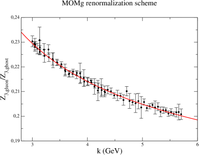
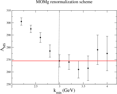
(a)	(b)

Figure 1: (a) Plot of the $\frac{Z_{3}(p^{2})}{\widetilde{Z}_{3}(p^{2})}$ for the best fit parameter $\Lambda_{\overline{\text{MS}}}=269(5)$ MeV. (b) The determination of the optimal window fit (from 3 GeV to $k_{\rm max}a\leq\pi/2$) results from the search for some “plateau” of $\Lambda_{\overline{\text{MS}}}$ when one changes the low bound of the fit window.

scheme	$\Lambda_{\overline{\text{MS}}}^{\text{2 loops}}$	$\chi^{2}$/d.o.f	$\Lambda_{\overline{\text{MS}}}^{\text{3 loops}}$	$\chi^{2}$/d.o.f	$\Lambda_{\overline{\text{MS}}}^{\text{4 loops}}$	$\chi^{2}$/d.o.f
$\widetilde{\text{MOM}_{g}}$	$324(6)$	$0.33$	$269(5)$	$0.34$	$282(6)$	$0.34$
$\widetilde{\text{MOM}_{c}}$	$351(6)$	$0.33$	$273(5)$	$0.34$	$291(6)$	$0.33$
$\widetilde{\text{MOM}_{c0}}$	$385(7)$	$0.33$	$281(5)$	$0.34$	$298(6)$	$0.33$

Table 2: The best-fitted values of $\Lambda_{\overline{\text{MS}}}$ for the three considered renormalisation schemes. As discussed in the text, $\widetilde{\text{MOM}_{g}}$ seems to be the one showing the best asymptotic behaviour.

In Fig. 2.(a) we show the evolution of the fitted parameter $\Lambda_{\overline{\text{MS}}}$ when changing the order of the perturbation theory used in the fitting formula. One can conclude from Fig. 2.(a) and App. A that $\widetilde{\text{MOM}_{g}}$ scheme at three loops gives the most stable results for $\Lambda_{\overline{\text{MS}}}$. It can also be seen from the ratio of four to three loops contributions (see Fig. 2.(b)) for the perturbative expansion of $\log{Z_{3}}$,

$$\ln(Z_{3})\ =\ r_{0}\ln(h_{R})+\sum_{i=1}r_{i}h_{R}^{i}\ ,$$ (17)

where the coefficients $r_{i}$ are to be computed from those in Eqs. (2.1-8) and $R$ stands for any renormalisation scheme ($R=\widetilde{\text{MOM}_{g}}$ in Fig. 2.(b)). The same is done for $\log{\widetilde{Z_{3}}}$.

According to our analysis, three loops seems to be the optimal order for asymptoticity. Indeed, the values of $\Lambda_{\overline{\text{MS}}}$ for the three considered renormalisation schemes practically match each other at three loops. Finally,

$$\Lambda_{\overline{\text{MS}}}=269(5)^{+12}_{-9}$$ (18)

could be presented as the result for the fits of the ratio of dressing functions to perturbative formulae, where we take into account the bias due to the choice of the fitting window (see Fig. 1.(b)  and App. A).

However, there are indications (App. A and [8]) that our present systematic uncertainty may be underestimated, and we prefer simply to quote $\Lambda_{\overline{\text{MS}}}\approx 270\text{ MeV}\ .$ This value is considerably smaller than the value of $\approx 320\text{ MeV}$ obtained by independent fits of dressing functions ([8]), and with fitting windows independently determined for each lattice sample (see Fig. 2.(a)). This argues in favour of presence of low-order non-perturbative corrections to the ghost and gluon propagators.

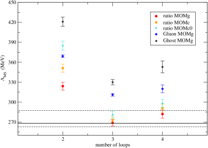
(a)	(b)

Figure 2: (a) Evolution of the parameter $\Lambda_{\overline{\text{MS}}}$, extracted from fits of the ratio Eq. (16) and propagators alone (rhombus and star markers, extracted from Tab.7 of [8]) to perturbative formulae, as function of the order of the perturbation theory. Only statistical error is quoted. (b) Ratio of four-loop to three-loop contributions (and of three-loop to two-loops for the sake of comparison) for the perturbative expansion of $\log{Z_{3}}$ and $\log{\widetilde{Z_{3}}}$ (in $\widetilde{\text{MOM}_{g}}$) in Eq. (17), plotted versus the momenta inside our fitting window.

3.3 Estimating the value of the $\langle A^{2}\rangle$ gluon condensate

Knowing $\Lambda_{\overline{\text{MS}}}$ we can fit ghost and gluon dressing functions using Eqs. (9,15). The free parameter in this case is $g_{R}^{2}\langle A^{2}\rangle$. According to the theoretical argument given in 2.2, the results obtained from these fits have to be compatible. We have performed this analysis for the rough value $\Lambda_{\overline{\text{MS}}}\approx 270\text{ MeV}$, (see Tab. 3). Indeed, we find that the resulting values agree. It is worth to emphasise the meaning of this result: a fully self-consistent description of gluon and ghost propagators computed from the same sample of lattice configuration (same $\Lambda_{\overline{\text{MS}}}$ and same $\langle A^{2}\rangle$) is obtained.

	$Z_{3}$	$\widetilde{Z_{3}}$
$g_{R}^{2}\langle A^{2}\rangle$ (GeV2)	2.7(4)	2.7(2)

Table 3: The best-fitted values of $g_{R}^{2}\langle A^{2}\rangle$ for $\widetilde{\text{MOM}_{g}}$ obtained from fitting lattice data to a three-loop perturbative formula + non-perturbative power correction with $\Lambda_{\overline{\text{MS}}}=270$ MeV. We only quote statistical errors.

The values of the gluon condensate presented in Tab. 3 are smaller than those obtained from the previous analysis of the gluon propagator [2]. The reason for this is the larger value of $\Lambda_{\overline{\text{MS}}}$ we have found. Had we taken $\Lambda_{\overline{\text{MS}}}\simeq 240$ MeV, we would obtain similar results to those previously presented. Of course, this discrepancy have to be included in the present systematical uncertainty of our analysis of the ghost propagator lattice data. However, the purpose of this paper is not to present a precise determination of the dimension-two gluon condensate, but only to show that ghost and gluon propagators analysis strongly indicates its existence. The precision could be improved by increasing the Monte-Carlo statistics and by performing new simulations at larger $\beta$.

Another source of discrepancy are renormalon-type contributions that can also be of the order of $\sim 1/q^{2}$. In fact, our OPE study does not include the analysis of such corrections. However, the numerical equality (cf. Tab.3) of $\sim 1/q^{2}$ power corrections at fixed $\Lambda_{\overline{\text{MS}}}$ suggests that the ratio (16) is free of such corrections, in agreement with the common belief that the renormalon ambiguities are compensated by condensate contributions. The estimate for $\Lambda_{\overline{\text{MS}}}$ obtained from this ratio is thus not affected by the renormalon-type contributions. But the dependence of the value of these corrections on $\Lambda_{\overline{\text{MS}}}$ speaks in favour of the presence of renormalon-type contributions in $Z_{3}$ and $\widetilde{Z_{3}}$ separately.

4 Conclusions

We have analysed non-perturbative low-order power corrections to the ghost propagator in Landau gauge pure Yang-Mills theory using OPE. We found that these corrections are the same as those for the gluon propagator at leading order. This means that their ratio does not contain low-order power corrections ($\sim 1/q^{2}$), and can be described (up to terms of order $\sim 1/q^{4}$) by the perturbation theory. Fitting the ratio of propagators calculated on the lattice we have extracted the $\Lambda_{\overline{\text{MS}}}$ parameter using three- and four-loop perturbation theory. The value $\Lambda_{\overline{\text{MS}}}\approx 270\text{ MeV}$ extracted from the ratio is quite small compared to the one obtained in fits of gluon and ghost propagator ($\Lambda^{\text{pert}}_{\overline{\text{MS}}}\approx 320\text{ MeV}$, [8]) separately. Indeed, $\Lambda_{\overline{\text{MS}}}\approx 270\text{ MeV}$ extracted from the ratio of ghost and gluon dressing functions is closer to the value calculated in the past with power-corrections taken into account ($\Lambda^{\text{with }A^{2}}_{\overline{\text{MS}}}\approx 250\text{ MeV}$, [3, 4]) than to the purely perturbative result . This study within perturbation theory confirms the validity of our OPE analysis, and argues in favour of a non-zero value of non-perturbative $A^{2}$-condensate. We are not able at the moment to give a precise value of the $A^{2}$-condensate using this strategy. More lattice data and detailed analysis of diverse systematic uncertainties are needed for this. But the method exposed in this letter can in principle be used for this purpose, both in quenched and unquenched cases.

Appendix A Appendix

In this Appendix we present results for $\Lambda_{\text{QCD}}$ extracted by fitting the ratio $\frac{\widetilde{Z}_{3}(p^{2})}{Z_{3}(p^{2})}$ using two, three and four-loop perturbation theory. But we do not mix data samples obtained in different lattice simulations. This allows to control the effects of several lattice artifacts and of the uncertainty on the lattice spacing calculation on the resulting value of $\Lambda_{\text{QCD}}$. Fits have been performed in $\widetilde{\text{MOM}_{c}},\widetilde{\text{MOM}_{c0}},\widetilde{\text{MOM}_{g}}$ renormalisation schemes (cf. Tab. 4,5,6,7,8,9). In each case we chose the best fit from several fitting windows, having the smallest $\chi^{2}/{\text{d.o.f.}}$; the statistical error corresponds to that fit. The systematic error is calculated from different fit windows.

One can see from these fits that the values for $\Lambda_{\overline{\text{MS}}}$ are small at three and four loops when fitting at energies $\geq 3\text{GeV}$. All results are rather stable in this domain, and thus the fitting of combined data from the simulations with different lattice spacings, presented in the main part of the present letter, is safe and well defined.

Fits at two loops

V	$\beta$	Left, GeV	Right,GeV	$a\Lambda^{(2)}_{\frac{\widetilde{Z}_{3}}{Z_{3}},\widetilde{\text{MOM}_{g}}}$	conversion to $\Lambda^{(2)\overline{\text{MS}}}$, MeV	$\chi 2/\text{d.o.f.}$
$16^{4}$	$6.0$	$2.54$	$4.32$	$529(17)^{+4~{}}_{-2~{}}$	$359(12)^{+2}_{-1~{}}$	$0.21$
$24^{4}$	$6.0$	$3.14$	$4.12$	$513(15)^{+16}_{-16}$	$348(10)^{+11}_{-11}$	$0.10$
$24^{4}$	$6.2$	$3.02$	$4.95$	$377(24)_{-11}$	$358(22)_{-10}$	$0.14$
$32^{4}$	$6.4$	$3.66$	$5.85$	$257(21)^{+1~{}}_{-4~{}}$	$325(26)^{+3}_{-5}$	$0.17$

Table 4: Perturbative fit of $\frac{\widetilde{Z}_{3}(p2)}{Z_{3}(p2)}$ at 2 loops in $\widetilde{\text{MOM}_{g}}$ scheme and further conversion to $\overline{\text{MS}}$

V	$\beta$	Left, GeV	Right,GeV	$a\Lambda^{(2)}_{\frac{\widetilde{Z}_{3}}{Z_{3}},\widetilde{\text{MOM}_{c}}}$	conversion to $\Lambda^{(2)\overline{\text{MS}}}$, MeV	$\chi 2/\text{d.o.f.}$
$16^{4}$	$6.0$	$2.15$	$4.12$	$445(6)_{-6~{}}$	$375(5)_{-5~{}}$	$0.14$
$24^{4}$	$6.0$	$3.14$	$4.12$	$398(53)^{+16}_{-1~{}}$	$335(45)^{+11}_{-1}$	$0.10$
$24^{4}$	$6.2$	$3.02$	$4.95$	$313(19)_{-22}$	$369(22)_{-26}$	$0.13$
$32^{4}$	$6.4$	$3.66$	$5.85$	$215(17)^{+2~{}}_{-2~{}}$	$337(26)^{+3}_{-3}$	$0.17$

Table 5: Perturbative fit of $\frac{\widetilde{Z}_{3}(p2)}{Z_{3}(p2)}$ at 2 loops in $\widetilde{\text{MOM}_{c}}$ scheme and further conversion to $\overline{\text{MS}}$

V	$\beta$	Left, GeV	Right,GeV	$a\Lambda^{(2)}_{\frac{\widetilde{Z}_{3}}{Z_{3}},\widetilde{\text{MOM}_{c0}}}$	conversion to $\Lambda^{(2)\overline{\text{MS}}}$, MeV	$\chi 2/\text{d.o.f.}$
$16^{4}$	$6.0$	$1.97$	$4.11$	$400(6)_{-5~{}}$	$413(6)_{-5~{}}$	$0.15$
$24^{4}$	$6.0$	$3.13$	$4.12$	$354(49)^{+26}$	$367(41)^{+27}$	$0.11$
$24^{4}$	$6.2$	$3.02$	$4.95$	$280(17)^{+1~{}}_{-12}$	$367(24)^{+1~{}}_{-17}$	$0.11$
$32^{4}$	$6.4$	$3.66$	$5.85$	$190(16)^{+2~{}}_{-3~{}}$	$366(30)^{+4}_{-6}$	$0.16$

Table 6: Perturbative fit of $\frac{\widetilde{Z}_{3}(p2)}{Z_{3}(p2)}$ at 2 loops in $\widetilde{\text{MOM}_{c0}}$ scheme and further conversion to $\overline{\text{MS}}$

Fits at three loops

V	$\beta$	Left, GeV	Right,GeV	$a\Lambda^{(3)}_{\frac{\widetilde{Z}_{3}}{Z_{3}},\widetilde{\text{MOM}_{c}}}$	conversion to $\Lambda^{(3)\overline{\text{MS}}}$, MeV	$\chi^{2}/\text{d.o.f.}$
$16^{4}$	$6.0$	$2.54$	$4.31$	$354(12)^{+5~{}}_{-5~{}}$	$297(10)^{+4~{}}_{-4~{}}$	$0.23$
$24^{4}$	$6.0$	$3.13$	$4.12$	$312(48)^{+30}$	$261(40)^{+25}$	$0.10$
$24^{4}$	$6.2$	$3.14$	$4.95$	$247(20)_{-22}$	$289(23)_{-26}$	$0.14$
26 $32^{4}$	$6.4$	$3.66$	$5.86$	$163(15)^{+2~{}}_{-1~{}}$	$254(24)^{+3~{}}_{-2~{}}$	$0.16$

Table 7: Perturbative fit of $\frac{\widetilde{Z}_{3}(p^{2})}{Z_{3}(p^{2})}$ at 3 loops in $\widetilde{\text{MOM}_{c}}$ scheme and further conversion to $\overline{\text{MS}}$

V	$\beta$	Left, GeV	Right,GeV	$a\Lambda^{(3)}_{\frac{\widetilde{Z}_{3}}{Z_{3}},\widetilde{\text{MOM}_{g}}}$	conversion to $\Lambda^{(3)\overline{\text{MS}}}$, MeV	$\chi^{2}/\text{d.o.f.}$
$16^{4}$	$6.0$	$2.06$	$3.44$	$453(18)_{-5}$	$307(12)_{-4}$	$0.16$
$24^{4}$	$6.0$	$2.06$	$3.53$	$451(16)^{+2}_{-10}$	$306(11)^{+1}_{-7}$	$0.1$
$24^{4}$	$6.2$	$2.80$	$4.81$	$295(20)^{+15}$	$282(19)^{+14}$	$0.13$
$32^{4}$	$6.4$	$3.79$	$5.59$	$216(25)_{-13}$	$270(31)_{-16}$	$0.13$

Table 8: Perturbative fit of $\frac{\widetilde{Z}_{3}(p^{2})}{Z_{3}(p^{2})}$ at 3 loops in $\widetilde{\text{MOM}_{g}}$ scheme and further conversion to $\overline{\text{MS}}$

V	$\beta$	Left, GeV	Right,GeV	$a\Lambda^{(3)}_{\frac{\widetilde{Z}_{3}}{Z_{3}},\widetilde{\text{MOM}_{c0}}}$	conversion to $\Lambda^{(3)\overline{\text{MS}}}$, MeV	$\chi^{2}/\text{d.o.f.}$
$16^{4}$	$6.0$	$2.16$	$3.53$	$312(11)_{-17}$	$323(11)_{-18}$	$0.11$
$24^{4}$	$6.0$	$3.21$	$4.11$	$252(47)^{+36}$	$260(48)^{+37}$	$0.10$
$24^{4}$	$6.2$	$3.13$	$4.95$	$205(16)_{-18}$	$297(23)_{-26}$	$0.14$
$32^{4}$	$6.4$	$3.66$	$5.86$	$136(12)^{+1~{}}_{-2~{}}$	$262(23)^{+2~{}}_{-2~{}}$	$0.17$

Table 9: Perturbative fit of $\frac{\widetilde{Z}_{3}(p^{2})}{Z_{3}(p^{2})}$ at 3 loops in $\widetilde{\text{MOM}_{c0}}$ scheme and further conversion to $\overline{\text{MS}}$

Fits at four loops

V	$\beta$	Left, GeV	Right,GeV	$a\Lambda^{(4)}_{\frac{\widetilde{Z}_{3}}{Z_{3}},\widetilde{\text{MOM}_{g}}}$	conversion to $\Lambda^{(4)\overline{\text{MS}}}$, MeV	$\chi 2/\text{d.o.f.}$
$16^{4}$	$6.0$	$-$	$-$	$-$	$-$	$-$
$24^{4}$	$6.0$	$3.14$	$4.12$	$365(13)^{+18}$	$248(8)^{+12}$	$0.10$
$24^{4}$	$6.2$	$3.02$	$4.95$	$288(17)^{+1~{}}_{-4~{}}$	$274(16)^{+1}_{-4}$	$0.13$
$32^{4}$	$6.4$	$3.66$	$5.85$	$199(15)^{+5~{}}$	$252(19)^{+6~{}}$	$0.17$

Table 10: Perturbative fit of $\frac{\widetilde{Z}_{3}(p2)}{Z_{3}(p2)}$ at 4 loops in $\widetilde{\text{MOM}_{g}}$ scheme and further conversion to $\overline{\text{MS}}$

V	$\beta$	Left, GeV	Right,GeV	$a\Lambda^{(4)}_{\frac{\widetilde{Z}_{3}}{Z_{3}},\widetilde{\text{MOM}_{c}}}$	conversion to $\Lambda^{(4)\overline{\text{MS}}}$, MeV	$\chi 2/\text{d.o.f.}$
$16^{4}$	$6.0$	$-$	$-$	$-$	$-$	$-$
$24^{4}$	$6.0$	$-$	$-$	$-$	$-$	$-$
$24^{4}$	$6.2$	$-$	$-$	$-$	$-$	$-$
$32^{4}$	$6.4$	$3.66$	$5.85$	$175(15)^{+1~{}}_{-2~{}}$	$274(23)^{+2}_{-4}$	$0.17$

Table 11: Perturbative fit of $\frac{\widetilde{Z}_{3}(p2)}{Z_{3}(p2)}$ at 4 loops in $\widetilde{\text{MOM}_{c}}$ scheme and further conversion to $\overline{\text{MS}}$

V	$\beta$	Left, GeV	Right,GeV	$a\Lambda^{(4)}_{\frac{\widetilde{Z}_{3}}{Z_{3}},\widetilde{\text{MOM}_{c0}}}$	conversion to $\Lambda^{(4)\overline{\text{MS}}}$, MeV	$\chi 2/\text{d.o.f.}$
$16^{4}$	$6.0$	$-$	$-$	$-$	$-$	$-$
$24^{4}$	$6.0$	$2.95$	$4.12$	$299(29)_{-26}$	$309(30)_{-27}$	$0.11$
$24^{4}$	$6.2$	$3.02$	$4.95$	$225(14)^{+1~{}}_{-4~{}}$	$326(20)^{+1}_{-6}$	$0.13$
$32^{4}$	$6.4$	$3.66$	$5.85$	$152(13)^{+1~{}}_{-2~{}}$	$293(25)^{+2~{}}_{-4~{}}$	$0.16$

Table 12: Perturbative fit of $\frac{\widetilde{Z}_{3}(p2)}{Z_{3}(p2)}$ at 4 loops in $\widetilde{\text{MOM}_{c0}}$ scheme and further conversion to $\overline{\text{MS}}$

References

- [1] K. G. Chetyrkin, S. Narison and V. I. Zakharov, Nucl. Phys. B 550 (1999) 353 [arXiv:hep-ph/9811275]. L. Stodolsky, P. van Baal and V. I. Zakharov, Phys. Lett. B 552 (2003) 214 [arXiv:hep-th/0210204];
- [2] Ph. Boucaud, A. Le Yaouanc, J.P. Leroy, J. Micheli, O. Pène, J. Rodriguez-Quintero, Phys. Lett. B493 (2000) 315.
- [3] Ph. Boucaud,A. Le Yaouanc, J.P. Leroy, J. Micheli, O. Pène, J. Rodriguez-Quintero, Phys. Rev. D63 (2001) 114003
- [4] P. Boucaud et al., JHEP 0004 (2000) 006 [arXiv:hep-ph/0003020]; F. De Soto and J. Rodriguez-Quintero, Phys. Rev. D 64 (2001) 114003 [arXiv:hep-ph/0105063]; P. Boucaud et al., Phys. Rev. D 66 (2002) 034504 [arXiv:hep-ph/0203119]; P. Boucaud et al., Phys. Rev. D 67 (2003) 074027 [arXiv:hep-ph/0208008].
- [5] D. Dudal, H. Verschelde and S. P. Sorella, Phys. Lett. B 555 (2003) 126 [arXiv:hep-th/0212182]; D. Dudal, R. F. Sobreiro, S. P. Sorella and H. Verschelde, [arXiv:hep-th/0502183].
- [6] K. I. Kondo, Phys. Lett. B 572 (2003) 210 [arXiv:hep-th/0306195].
- [7] F. V. Gubarev, L. Stodolsky and V. I. Zakharov, Phys. Rev. Lett. 86 (2001) 2220 [arXiv:hep-ph/0010057]. K. I. Kondo, Phys. Lett. B 514 (2001) 335 [arXiv:hep-th/0105299].
- [8] Ph. Boucaud, J.P. Leroy, A. Le Yaouanc, A.Y. Lokhov, J. Micheli, O. Pene, J. Rodriguez-Quintero, C. Roiesnel, [arXiv:hep-lat/0506031]
- [9] K. G. Chetyrkin, Nucl. Phys. B 710 (2005) 499 [arXiv:hep-ph/0405193];
- [10] M. Czakon, Nucl. Phys. B 710 (2005) 485 [arXiv:hep-ph/0411261].
- [11] D. Becirevic, P. Boucaud, J. P. Leroy, J. Micheli, O. Pene, J. Rodriguez-Quintero and C. Roiesnel, Phys. Rev. D 60 (1999) 094509 [arXiv:hep-ph/9903364].
- [12] D. Becirevic, P. Boucaud, J. P. Leroy, J. Micheli, O. Pene, J. Rodriguez-Quintero and C. Roiesnel, Phys. Rev. D 61 (2000) 114508 [arXiv:hep-ph/9910204].
- [13] G. Grunberg, Phys. Rev. D 29 (1984) 2315.
- [14] K. G. Chetyrkin and A. Retey, [arXiv:hep-ph/0007088].
- [15] T. van Ritbergen, J. A. M. Vermaseren and S. A. Larin, Phys. Lett. B 400 (1997) 379 [arXiv:hep-ph/9701390].
- [16] R. Wilson, Phys. Rev. 179 (1969) 1499.
- [17] M.A. Shifman, A.I. Vainshtein, V.I. Zakharov, Nucl. Phys. B147 (1979) 385,447,519; M.A. Shifman, A.I. Vainshtein, M.B. Voloshin, V.I. Zakharov, Phys. Lett. B77 (1978) 80;
-
[18]
J. C. Taylor,
Nuclear Physics B
Volume 33, Issue 2 , 1 November 1971, Pages 436-444
A. A. Slavnov, Theor. Math. Phys. 10 (1972) 99 [Teor. Mat. Fiz. 10 (1972) 153]. - [19] F. De Soto and J. Rodriguez-Quintero, Phys. Rev. D 64 (2001) 114003 [arXiv:hep-ph/0105063].