SWAT 05-435

Continuum and lattice meson spectral functions
at nonzero momentum and high temperature

Abstract

We analyse discretization effects in the calculation of high-temperature meson spectral functions at nonzero momentum and fermion mass on the lattice. We do so by comparing continuum and lattice spectral functions in the infinite temperature limit. Complete analytical results for the spectral densities in the continuum are presented, along with simple expressions for spectral functions obtained with Wilson and staggered fermions on anisotropic lattices. We comment on the use of local and point split currents.

1 Introduction

Motivated by the experimental progress in relativistic heavy ion collisions and the recreation of the quark gluon plasma, several questions have received substantial attention in the past few years. What happens to hadrons in the deconfined quark-gluon plasma? Do bound states persist? What is rate of photon and dilepton production from a hot QGP? How effectively are energy-momentum and charge transported? How long, or rather how short, are the typical relaxation times for hydrodynamic fluctuations?

Since this information is encoded in spectral functions, it is prohibitively difficult to access it directly from euclidean correlators obtained with lattice QCD, due to the intricacy of performing the analytical continuation from imaginary to real time. However, recent progress has been made by applying the Maximal Entropy Method (MEM) [1] to this problem. An (incomplete) list of high temperature studies includes the possible survival of hadronic bound states in the deconfined quark-gluon plasma [2, 3, 4], thermal dilepton rates [5], and transport coefficients [6].

In a spectral function investigation, the low-energy region $\omega\lesssim T$ is of particular interest, since it is expected to be the most affected by nonperturbative medium effects. However, the reconstruction of spectral functions at small energies $\omega\ll T$ is hindered by the insensitivity of euclidean correlators to details of spectral functions at these energies [9]. This is especially important for the calculation of transport coefficients where by definition the interest is in the limiting value of current-current spectral densities as $\omega\to 0$. Experience with the reconstruction of spectral densities in the low-energy region can be obtained by studying the simpler (but still nontrivial) problem of meson spectral functions at nonzero momentum above the deconfinement transition. Due to e.g. the scattering of quarks with gauge bosons below the lightcone (Landau damping), these spectral functions are expected to have a nontrivial structure. Since in the confined phase one expects to find mesons moving relative to the heatbath, described by simple quasiparticle spectral functions, increasing the temperature from below to above the transition temperature should result in a drastic change in those spectral functions.

Our aim in this paper is to provide a reference point for such an analysis on the lattice in the infinite temperature limit. It is therefore similar in spirit as Ref. [10], in which a study at zero momentum was performed. The paper is organized as follows. In the next section we give complete analytical expressions for continuum meson spectral functions at nonzero momentum and fermion mass in the infinite temperature limit and discuss several features. In Section 3 we derive simple expressions for meson spectral functions for Wilson and staggered lattice fermions. We briefly comment on the value of the euclidean correlator at the midpoint and on the use of local and point split currents. The main results are shown in Section 4, where we contrast spectral functions obtained with Wilson and staggered fermions with the continuum results. Section 5 contains a short summary.

2 Continuum

We consider meson spectral functions with quantum numbers $H$, defined as

$$\rho_{H}(t,{\mathbf{x}})=\langle[J_{H}(t,{\mathbf{x}}),J_{H}^{\dagger}(0,{\mathbf{0}})]\rangle,$$ (1)

with $J_{H}(\tau,{\mathbf{x}})=\bar{q}(\tau,{\mathbf{x}})\Gamma_{H}q(\tau,{\mathbf{x}})$ and $\Gamma_{H}=\{{1\!\!1},\gamma_{5},\gamma^{\mu},\gamma^{\mu}\gamma_{5}\}$. They are related to euclidean correlation functions,

$$G_{H}(\tau,{\mathbf{x}})=\langle J_{H}(\tau,{\mathbf{x}})J_{H}^{\dagger}(0,{\mathbf{0}})\rangle,$$ (2)

via the standard integral relation

$$G_{H}(\tau,{\mathbf{p}})=\int_{0}^{\infty}\frac{d\omega}{2\pi}\,K(\tau,\omega)\rho_{H}(\omega,{\mathbf{p}}),$$ (3)

with the kernel

$$K(\tau,\omega)=\frac{\cosh[\omega(\tau-1/2T)]}{\sinh(\omega/2T)}=e^{\omega\tau}n_{B}(\omega)+e^{-\omega\tau}\left[1+n_{B}(\omega)\right],$$ (4)

where $n_{B}(\omega)=1/(e^{\omega/T}-1)$ is the Bose distribution. At lowest order in the loop expansion, the euclidean correlators read in momentum space

$$G_{H}(P)=-\,\mbox{$\sum$}\int_{K}{\mathrm{tr}}\,S(K)\Gamma_{H}S(P+K)\gamma^{0}\Gamma_{H}^{\dagger}\gamma^{0},$$ (5)

where $P=(i\omega_{n},{\mathbf{p}})$ with $\omega_{n}=2\pi nT$ ($n\in\mathbb{Z}$) the Matsubara frequency in the imaginary-time formalism, and

$$\,\mbox{$\sum$}\int_{K}=T\sum_{n}\int_{\mathbf{k}},\;\;\;\;\;\;\;\;\;\;\;\;\int_{\mathbf{k}}=\int\frac{d^{3}k}{(2\pi)^{3}}.$$ (6)

The fermion propagators are given by

$$S(K)=\frac{-1}{i\tilde{\omega}_{n}\gamma^{0}-\boldsymbol{\gamma}\cdot{\mathbf{k}}-m}=-\int_{-\infty}^{\infty}\frac{d\omega}{2\pi}\frac{\rho_{F}(\omega,{\mathbf{k}})}{i\tilde{\omega}_{n}-\omega},$$ (7)

where $\tilde{\omega}_{n}=(2n+1)\pi T$ ($n\in\mathbb{Z}$) is a fermionic Matsubara frequency and $\rho_{F}(\omega,{\mathbf{k}})$ the spectral density of the fermion,

$$\rho_{F}(K)=\left(/\!\!\!\!K+m\right)\rho(K)=\left(/\!\!\!\!K+m\right)2\pi\,\mbox{sgn}(k^{0})\delta(k_{0}^{2}-\omega_{\mathbf{k}}^{2}),$$ (8)

with $\omega_{\mathbf{k}}=\sqrt{{\mathbf{k}}^{2}+m^{2}}$.

Using the spectral representation for the fermion propagators, it is straightforward to arrive at

$$\rho_{H}(P)= 2{\mathrm{Im}}\,G_{H}(i\omega_{n}\to\omega+i0^{+},{\mathbf{p}})$$

$$= N_{c}\int_{{\mathbf{k}},k^{0}}{\mathrm{tr}}\,(/\!\!\!\!K+m)\Gamma_{H}(/\!\!\!\!R+m)\gamma^{0}\Gamma_{H}^{\dagger}\gamma^{0}\,\rho(K)\rho(R)\left[n_{F}(k^{0})-n_{F}(r^{0})\right],$$ (9)

with $P=(\omega,{\mathbf{p}})$, $R=P+K$ and $n_{F}(\omega)=1/(e^{\omega/T}+1)$ is the Fermi distribution.

To facilitate the comparison with the lattice expressions below, we give here the result with the $k^{0}$ integral performed,

$$\rho_{H}(P)= 2\pi N_{c}\int_{\mathbf{k}}\bigg{\{}\left(a_{H}^{(1)}+a_{H}^{(2)}\frac{{\mathbf{k}}\cdot{\mathbf{r}}}{\omega_{\mathbf{k}}\omega_{\mathbf{r}}}+a_{H}^{(3)}\frac{m^{2}}{\omega_{\mathbf{k}}\omega_{\mathbf{r}}}\right)\left[n_{F}(\omega_{\mathbf{k}})-n_{F}(\omega_{\mathbf{r}})\right]\delta(\omega+\omega_{\mathbf{k}}-\omega_{\mathbf{r}})$$ (10)

$$+\left(a_{H}^{(1)}-a_{H}^{(2)}\frac{{\mathbf{k}}\cdot{\mathbf{r}}}{\omega_{\mathbf{k}}\omega_{\mathbf{r}}}-a_{H}^{(3)}\frac{m^{2}}{\omega_{\mathbf{k}}\omega_{\mathbf{r}}}\right)\left[1-n_{F}(\omega_{\mathbf{k}})-n_{F}(\omega_{\mathbf{r}})\right]\delta(\omega-\omega_{\mathbf{k}}-\omega_{\mathbf{r}})$$

$$-(\omega\to-\omega)\bigg{\}}.$$

The first line corresponds to scattering and contributes only below the lightcone ($\omega^{2}<p^{2}$, Landau damping), while the second line corresponds to decay, contributing above threshold ($\omega^{2}>p^{2}+4m^{2}$). The coefficients $a_{H}^{(i)}$ arise from the three nonzero traces over the gamma matrices in Eq. (9) and depend on the channel under consideration. They are listed in Table 1.

	$\Gamma_{H}$	$a_{H}^{(1)}$	$a_{H}^{(2)}$	$a_{H}^{(3)}$
$\rho_{\rm S}$	${1\!\!1}$	$1$	$-1$	$1$
$\rho_{\rm PS}$	$\gamma_{5}$	$1$	$-1$	$-1$
$\rho^{00}$	$\gamma^{0}$	$1$	$1$	$1$
$\rho^{ii}$	$\gamma^{i}$	$3$	$-1$	$-3$
$\rho_{\rm V}$	$\gamma^{\mu}$	$2$	$-2$	$-4$
$\rho^{00}_{5}$	$\gamma^{0}\gamma_{5}$	$1$	$1$	$-1$
$\rho^{ii}_{5}$	$\gamma^{i}\gamma_{5}$	$3$	$-1$	$3$
$\rho_{\rm A}$	$\gamma^{\mu}\gamma_{5}$	$2$	$-2$	$4$

Table 1: Coefficients $a_{H}^{(i)}$ for free spectral functions in different channels $H$. In the case of $\gamma^{i}$ and $\gamma^{i}\gamma_{5}$, the sum is taken over $i=1,2,3$. We defined $\rho_{\rm V}=-g_{\mu\nu}\rho^{\mu\nu}$ and $\rho_{\rm A}=-g_{\mu\nu}\rho^{\mu\nu}_{5}$.

The remaining integrals can be performed as well. In terms of

$$\bar{p}_{\pm}=\frac{1}{2}\left[\omega\pm p\beta(P)\right],\;\;\;\;\;\;\;\;\beta(P)=\sqrt{1-\frac{4m^{2}}{s}},\;\;\;\;\;\;\;\;s=\omega^{2}-p^{2},$$ (11)

the final expression in the continuum reads

$$\rho_{H}(P)= \Theta(s-4m^{2})\frac{N_{c}T^{2}}{\pi}\bigg{\{}$$ (12)

$$\frac{\beta(P)}{24T^{2}}\left[\left(3\omega^{2}-p^{2}\beta^{2}(P)\right)a_{H}^{(1)}+\left(3p^{2}-(3\omega^{2}-2p^{2})\beta^{2}(P)\right)a_{H}^{(2)}-12m^{2}a_{H}^{(3)}\right]$$

$$+\frac{1}{4pT}\left[\left(\omega^{2}-p^{2}\beta^{2}(P)\right)a_{H}^{(1)}+\left(p^{2}-\omega^{2}\beta^{2}(P)\right)a_{H}^{(2)}-4m^{2}a_{H}^{(3)}\right]\ln\frac{1+e^{-{\bar{p}_{+}}/T}}{1+e^{-{\bar{p}_{-}}/T}}$$

$$+\left(a_{H}^{(1)}+a_{H}^{(2)}\right)\Big{(}\beta(P)\left[{\rm Li}_{2}(-e^{-{\bar{p}_{+}}/T})+{\rm Li}_{2}(-e^{-{\bar{p}_{-}}/T})\right]$$

$$\hskip 85.35826pt+\frac{2T}{p}\left[{\rm Li}_{3}(-e^{-{\bar{p}_{+}}/T})-{\rm Li}_{3}(-e^{-{\bar{p}_{-}}/T})\right]\Big{)}\bigg{\}}$$

$$+\Theta(-s)\frac{N_{c}T^{2}}{\pi}\bigg{\{}\frac{1}{4pT}\left[\left(\omega^{2}-p^{2}\beta^{2}(P)\right)a_{H}^{(1)}+\left(p^{2}-\omega^{2}\beta^{2}(P)\right)a_{H}^{(2)}-4m^{2}a_{H}^{(3)}\right]$$

$$\ln\frac{1+e^{-{\bar{p}_{+}}/T}}{1+e^{{\bar{p}_{-}}/T}}+\left(a_{H}^{(1)}+a_{H}^{(2)}\right)\Big{(}\beta(P)\left[{\rm Li}_{2}(-e^{-{\bar{p}_{+}}/T})-{\rm Li}_{2}(-e^{{\bar{p}_{-}}/T})\right]$$

$$\hskip 156.49014pt+\frac{2T}{p}\left[{\rm Li}_{3}(-e^{-{\bar{p}_{+}}/T})-{\rm Li}_{3}(-e^{{\bar{p}_{-}}/T})\right]\Big{)}\bigg{\}}.$$

We now discuss several features. First consider the asymptotic behaviour at large $\omega$. We find that all spectral functions increase with $\omega^{2}$,

$$\lim_{\omega\to\infty}\rho_{H}(P)=\Theta(s-4m^{2})\frac{N_{c}}{8\pi}\omega^{2}\left(a_{H}^{(1)}-a_{H}^{(2)}\right),$$ (13)

as expected from naive dimensional arguments, except when there is a cancellation. This happens for $\Gamma_{H}=\gamma^{0},\gamma^{0}\gamma_{5}$, for which we find instead

$$\lim_{\omega\to\infty}\rho^{00}(P)= \Theta(s-4m^{2})\frac{N_{c}}{6\pi}p^{2},$$

$$\lim_{\omega\to\infty}\rho^{00}_{5}(P)= \Theta(s-4m^{2})\frac{N_{c}}{6\pi}\left(p^{2}+6m^{2}\right).$$ (14)

For the vector current this behaviour can be understood from current conservation $\partial_{\mu}j^{\mu}=0$. Since at large $\omega$ the effect of finite temperature is exponentially suppressed, we may use the zero temperature decomposition,

$$\rho^{\mu\nu}(P)=2{\mathrm{Im}}\,\Pi^{\mu\nu}_{R}(P)=2\left(P^{2}g^{\mu\nu}-P^{\mu}P^{\nu}\right){\mathrm{Im}}\,\Pi_{R}(P^{2}),$$ (15)

which explains the behaviour above. Current conservation also relates the other components of $\rho^{\mu\nu}$,

$$\omega\rho^{00}(P)=p^{i}\rho^{i0}(P),\;\;\;\;\;\;\;\;\omega\rho^{0j}(P)=p^{i}\rho^{ij}(P),\;\;\;\;\;\;\;\;\omega^{2}\rho^{00}(P)=p^{i}p^{j}\rho^{ij}(P).$$ (16)

Since the axial vector current is not conserved,

$$\partial_{\mu}j^{\mu}_{5}=2mj_{5}+\mbox{anomaly},$$ (17)

similar relations do not hold for $\rho_{5}^{\mu\nu}$. However, in the free case considered here, we find

$$\omega^{2}\rho_{5}^{00}(\omega,{\mathbf{0}})=4m^{2}\rho_{\rm PS}(\omega,{\mathbf{0}}).$$ (18)

Any deviation from this is therefore due to the U(1)_A anomaly.

In the zero momentum limit, the spectral functions reduce to

$$\rho_{H}(\omega,{\mathbf{0}})=\Theta(\omega^{2}-4m^{2})\frac{N_{c}}{8\pi\omega}\sqrt{\omega^{2}-4m^{2}}\left[1-2n_{F}(\omega/2)\right]\Big{[}\omega^{2}\left(a_{H}^{(1)}-a_{H}^{(2)}\right)$$

$$+4m^{2}\left(a_{H}^{(2)}-a_{H}^{(3)}\right)\Big{]}+2\pi\omega\delta(\omega)N_{c}\left[\left(a_{H}^{(1)}+a_{H}^{(2)}\right)I_{1}+\left(a_{H}^{(2)}-a_{H}^{(3)}\right)I_{2}\right],$$ (19)

with

$$I_{1}=-2\int_{\mathbf{k}}n^{\prime}_{F}(\omega_{\mathbf{k}}),\;\;\;\;\;\;\;\;\;\;\;\;I_{2}=-2\int_{\mathbf{k}}\frac{k^{2}}{\omega_{\mathbf{k}}^{2}}n^{\prime}_{F}(\omega_{\mathbf{k}}).$$ (20)

In the massless case $I_{1}=I_{2}=T^{2}/6$. The term proportional to $\omega\delta(\omega)$ is all that remains from the scattering contribution below the lightcone in Eq. (10). It gives a $\tau$ independent contribution to the euclidean correlator since the kernel $K(\tau,\omega)\sim 2T/\omega$ for small $\omega$. In particular, charge conservation dictates the form of $\rho^{00}$ and $G^{00}$ at zero momentum,

$$\rho^{00}(\omega,{\mathbf{0}})=2\pi\chi\omega\delta(\omega),\hskip 56.9055ptG^{00}(\tau,{\mathbf{0}})=T\chi,$$ (21)

which is not altered by interactions, although the value of the charge susceptibility $\chi$ is. At the order computed here, $\chi=2N_{c}I_{1}$. For completeness we give here the euclidean correlator at zero momentum and mass

$$G_{H}(\tau,{\mathbf{0}})=\frac{N_{c}T^{3}}{6}\left[a_{H}^{(1)}+a_{H}^{(2)}+\frac{3}{2}\left(a_{H}^{(1)}-a_{H}^{(2)}\right)\frac{3u+u\cos(2u)-2\sin(2u)}{\sin^{3}u}\right],$$ (22)

where $u=2\pi T(\tau-1/2T)$.

Finally, it follows from the spectral decomposition

$$\rho_{H}(P)=\frac{1}{Z}\sum_{n,m}|\langle n|J_{H}(0)|m\rangle|^{2}(2\pi)^{4}\delta^{4}(P+P_{n}-P_{m})\left(e^{-p^{0}_{n}/T}-e^{-p^{0}_{m}/T}\right),$$ (23)

where $Z$ is the partition function, that all spectral functions for a single current $J_{H}$ are odd and positive semi-definite for positive argument, i.e. $\omega\rho_{H}(\omega,{\mathbf{p}})\geq 0$. Obviously, spectral functions that are defined as the difference between such spectral functions, such as $\rho_{\rm V}=\rho^{ii}-\rho^{00}$ and $\rho_{\rm A}=\rho^{ii}_{5}-\rho^{00}_{5}$ can turn negative. Indeed, it is easy to see that $\rho_{\rm V}(\omega,{\mathbf{p}})$ is negative for small $\omega$ if $p^{2}<2m^{2}$. All other spectral functions increase linearly with $\omega$ for small $\omega$ and nonzero ${\mathbf{p}}$.

Although not the topic of this paper, we briefly mention how corrections due to interactions appear at very high temperature. First of all, for soft momentum $|{\mathbf{p}}|\sim\omega\sim gT$, a hard thermal loop [11] calculation is needed, see e.g. Refs. [12, 13, 14] for such studies. The gap in the spectrum for $p^{2}<\omega^{2}<p^{2}+4m^{2}$ is filled when two loop diagrams are included, due to e.g. bremsstrahlung [15]. Around the lightcone the loop expansion breaks down due to the Landau-Pomeranchuk-Migdal effect and an infinite series of ladder diagrams contribute at leading order in the strong coupling constant [16, 17]. Finally for very soft momenta and energies, the structure of current-current spectral functions is determined by general hydrodynamical considerations [18]. So far a diagrammatic calculation in this regime has been carried out only in the case of the spatial vector spectral function $\rho^{ii}(\omega,{\mathbf{0}})$ in the limit of exactly zero momentum and vanishing energy $\omega\to 0$, which is relevant for the electrical conductivity: see Refs. [19, 20] for details on the weak coupling result at leading-logarithmic order and Ref. [21] for the large $N_{f}$ result.

3 Lattice

3.1 Wilson fermions

In this section we derive expressions for meson spectral functions on a lattice with $N_{\sigma}^{3}\times N_{\tau}$ sites. The lattice spacing is denoted with $a$ in the spatial directions and with $a_{\tau}$ in the temporal direction, $\xi=a/a_{\tau}$ is the anisotropy parameter. The temperature is related to the extent in the imaginary time direction, $T=1/(N_{\tau}a_{\tau})$. We start with standard Wilson fermions. The lattice fermion propagator (with coefficients $r_{4},r_{\rm space}=r$) reads

$$S(K)=\frac{-i\gamma_{4}\sin k_{4}-i{\cal K}_{\mathbf{k}}+r_{4}\left(1-\cos k_{4}\right)+{\cal M}_{\mathbf{k}}}{\sin^{2}k_{4}+{\cal K}^{2}_{\mathbf{k}}+\left[r_{4}\left(1-\cos k_{4}\right)+{\cal M}_{\mathbf{k}}\right]^{2}},$$ (24)

where

$${\cal K}_{\mathbf{k}}=\frac{1}{\xi}\sum_{i=1}^{3}\gamma_{i}\sin k_{i},\;\;\;\;\;\;\;\;\;\;\;\;{\cal M}_{\mathbf{k}}=\frac{1}{\xi}\left[r\sum_{i=1}^{3}\left(1-\cos k_{i}\right)+m\right].$$ (25)

We use periodic boundary conditions in space, $k_{i}=2\pi n_{i}/N_{\sigma}$ with $n_{i}=-N_{\sigma}/2+1,-N_{\sigma}/2+2,\ldots,N_{\sigma}/2-1,N_{\sigma}/2$ for $i=1,2,3$, and antiperiodic boundary conditions in imaginary time, $k_{4}=\pi(2n_{4}+1)/N_{\tau}$ with $n_{4}=-N_{\tau}/2+1,-N_{\tau}/2+2,\ldots,N_{\tau}/2-1,N_{\tau}/2$.

To make a smooth connection with the expressions in the continuum we follow Ref. [10] and use the mixed representation of Carpenter and Baillie [22]

$$S(\tau,{\mathbf{k}})=\gamma_{4}S_{4}(\tau,{\mathbf{k}})+\sum_{i=1}^{3}\gamma_{i}S_{i}(\tau,{\mathbf{k}})+{1\!\!1}S_{u}(\tau,{\mathbf{k}}).$$ (26)

In order to avoid the doubler in the time direction, we proceed with $r_{4}=1$, so that (for $0\leq\tau<1/T$)

$$S_{4}(\tau,{\mathbf{k}})= S_{4}({\mathbf{k}})\cosh(\tilde{\tau}E_{\mathbf{k}}),$$

$$S_{i}(\tau,{\mathbf{k}})= S_{i}({\mathbf{k}})\sinh(\tilde{\tau}E_{\mathbf{k}}),$$

$$S_{u}(\tau,{\mathbf{k}})= S_{u}({\mathbf{k}})\sinh(\tilde{\tau}E_{\mathbf{k}})-\frac{\delta_{\tau 0}}{2(1+{\cal M}_{\mathbf{k}})}.$$ (27)

Here $\tilde{\tau}=\tau-1/2T$ and

$$S_{4}({\mathbf{k}})= \frac{\sinh\left(E_{\mathbf{k}}/\xi\right)}{2{\cal E}_{\mathbf{k}}\cosh(E_{\mathbf{k}}/2T)},$$

$$S_{i}({\mathbf{k}})= \frac{1}{\xi}\frac{i\sin k_{i}}{2{\cal E}_{\mathbf{k}}\cosh(E_{\mathbf{k}}/2T)},$$

$$S_{u}({\mathbf{k}})= -\frac{1-\cosh\left(E_{\mathbf{k}}/\xi\right)+{\cal M}_{\mathbf{k}}}{2{\cal E}_{\mathbf{k}}\cosh(E_{\mathbf{k}}/2T)},$$ (28)

with ${\cal E}_{\mathbf{k}}=(1+{\cal M}_{\mathbf{k}})\sinh\left(E_{\mathbf{k}}/\xi\right)$. The single particle energy $E_{\mathbf{k}}$ is determined by

$$\cosh\left(E_{\mathbf{k}}/\xi\right)=1+\frac{{\cal K}_{\mathbf{k}}^{2}+{\cal M}_{\mathbf{k}}^{2}}{2(1+{\cal M}_{\mathbf{k}})}.$$ (29)

The final term in $S_{u}(\tau,{\mathbf{k}})$ is the sole remnant of the nonpropagating time doubler; below we consider $0<\tau<1/T$. The propagator satisfies $S(-\tau,{\mathbf{k}})=\gamma_{5}S^{\dagger}(\tau,{\mathbf{k}})\gamma_{5}$.

The correlators we are interested in are of the form

$$G_{H}(\tau,{\mathbf{p}})=-\frac{N_{c}}{L^{3}}\sum_{\mathbf{k}}{\mathrm{tr}}\,S(\tau,{\mathbf{k}})\Gamma_{H}S(-\tau,{\mathbf{r}})\Gamma_{H},$$ (30)

where again ${\mathbf{r}}={\mathbf{p}}+{\mathbf{k}}$. Inserting Eq. (26) gives the euclidean correlator

$$G_{H}(\tau,{\mathbf{p}})=\frac{4N_{c}}{L^{3}}\sum_{\mathbf{k}}\Big{[}a_{H}^{(1)}S_{4}(\tau,{\mathbf{k}})S_{4}^{\dagger}(\tau,{\mathbf{r}})-a_{H}^{(2)}\sum_{i}S_{i}(\tau,{\mathbf{k}})S_{i}^{\dagger}(\tau,{\mathbf{r}})$$

$$-a_{H}^{(3)}S_{u}(\tau,{\mathbf{k}})S_{u}^{\dagger}(\tau,{\mathbf{r}})\Big{]},$$ (31)

where the coefficients $a_{H}^{(i)}$ are the same as before (see Table 1).

We will now extract the spectral functions in a form that closely resembles the continuum expressions. In the terms $SS^{\dagger}$ we encounter products of hyperbolic functions. These can be written as

$$\sinh(\tilde{\tau}E_{\mathbf{k}})\sinh(\tilde{\tau}E_{\mathbf{r}})=\frac{1}{4}\int_{-\infty}^{\infty}d\omega\cosh(\omega\tilde{\tau})\Big{[}\delta(\omega-E_{\mathbf{k}}-E_{\mathbf{r}})+\delta(\omega+E_{\mathbf{k}}+E_{\mathbf{r}})$$

$$-\delta(\omega-E_{\mathbf{k}}+E_{\mathbf{r}})-\delta(\omega+E_{\mathbf{k}}-E_{\mathbf{r}})\Big{]},$$ (32)

and similarly for the product of two hyperbolic cosines. Noting that the factor $\cosh(\omega\tilde{\tau})$ is the sole place with $\tau$ dependence and that it is of the same form as in the kernel (4), it is straightforward to write the above expression for $G_{H}(\tau,{\mathbf{p}})$ as

$$G_{H}(\tau,{\mathbf{p}})=\int_{0}^{\infty}\frac{d\omega}{2\pi}\,K(\tau,\omega)\rho^{\rm Wilson}_{H}(\omega,{\mathbf{p}}),$$ (33)

and read off the expressions for the lattice spectral functions,

$$\rho^{\rm Wilson}_{H}(P)=\frac{4\pi N_{c}}{L^{3}}\sum_{\mathbf{k}}\sinh\left(\frac{\omega}{2T}\right)\bigg{\{}$$

$$\;\;\;\;\;\;\;\;\bigg{[}a_{H}^{(1)}S_{4}({\mathbf{k}})S^{\dagger}_{4}({\mathbf{r}})+a_{H}^{(2)}\sum_{i}S_{i}({\mathbf{k}})S^{\dagger}_{i}({\mathbf{r}})+a_{H}^{(3)}S_{u}({\mathbf{k}})S^{\dagger}_{u}({\mathbf{r}})\bigg{]}\delta(\omega+E_{\mathbf{k}}-E_{\mathbf{r}})$$

$$\;\;\;\;\;\;\;\;+\bigg{[}a_{H}^{(1)}S_{4}({\mathbf{k}})S^{\dagger}_{4}({\mathbf{r}})-a_{H}^{(2)}\sum_{i}S_{i}({\mathbf{k}})S^{\dagger}_{i}({\mathbf{r}})-a_{H}^{(3)}S_{u}({\mathbf{k}})S^{\dagger}_{u}({\mathbf{r}})\bigg{]}\delta(\omega-E_{\mathbf{k}}-E_{\mathbf{r}})$$

$$\;\;\;\;\;\;\;\;+(\omega\to-\omega)\bigg{\}}.$$ (34)

This result can be directly compared with the continuum expression (10), using Eq. (28) and realizing that

$$\frac{\sinh(\omega/2T)}{\cosh(E_{\mathbf{k}}/2T)\cosh(E_{\mathbf{r}}/2T)}=\begin{cases}2\left[n_{F}(E_{\mathbf{k}})-n_{F}(E_{\mathbf{r}})\right]&\;\;{\rm if}\;\;\omega=E_{\mathbf{r}}-E_{\mathbf{k}},\\ 2\left[1-n_{F}(E_{\mathbf{k}})-n_{F}(E_{\mathbf{r}})\right]&\;\;{\rm if}\;\;\omega=E_{\mathbf{r}}+E_{\mathbf{k}}.\end{cases}$$ (35)

3.2 Staggered fermions

In the case of staggered fermions we perform the analysis with naive fermions, since this leads to equivalent results [23]. Taking therefore $r_{4}=r_{\rm space}=0$ yields the fermion propagator (26) with

$$S_{4}(\tau,{\mathbf{k}})= S_{4}({\mathbf{k}})\left(1-(-1)^{\tau/a_{\tau}}\right)\cosh(\tilde{\tau}E_{\mathbf{k}}),$$

$$S_{i}(\tau,{\mathbf{k}})= S_{i}({\mathbf{k}})\left(1+(-1)^{\tau/a_{\tau}}\right)\sinh(\tilde{\tau}E_{\mathbf{k}}),$$

$$S_{u}(\tau,{\mathbf{k}})= S_{u}({\mathbf{k}})\left(1+(-1)^{\tau/a_{\tau}}\right)\sinh(\tilde{\tau}E_{\mathbf{k}}),$$ (36)

where $S_{4}({\mathbf{k}})$ and $S_{i}({\mathbf{k}})$ are as in Eq. (28) with ${\cal E}_{\mathbf{k}}=\cosh\left(E_{\mathbf{k}}/\xi\right)\sinh\left(E_{\mathbf{k}}/\xi\right)$, and

$$S_{u}(\tau,{\mathbf{k}})=-\frac{1}{\xi}\frac{m}{2{\cal E}_{\mathbf{k}}\cosh(E_{\mathbf{k}}/2T)}.$$ (37)

The single particle energy $E_{\mathbf{k}}$ is now determined by

$$\cosh\left(E_{\mathbf{k}}/\xi\right)=\sqrt{1+{\cal K}_{\mathbf{k}}^{2}+(m/\xi)^{2}}.$$ (38)

Using the same steps as before, the euclidean meson correlator takes again the form (LABEL:eqG) and can be written in a spectral representation as

$$G_{H}(\tau,{\mathbf{p}})=2\int_{0}^{\infty}\frac{d\omega}{2\pi}K(\tau,\omega)\left[\rho_{H}^{\rm naive}(\omega,{\mathbf{p}})-(-1)^{\tau/a_{\tau}}\tilde{\rho}_{H}^{\rm naive}(\omega,{\mathbf{p}})\right],$$ (39)

with the same kernel as above.

The desired spectral function $\rho_{H}^{\rm naive}(\omega,{\mathbf{p}})$ is exactly as in Eq. (34), whereas the staggered partner $\tilde{\rho}_{H}^{\rm naive}(\omega,{\mathbf{p}})$ has the same form but with coefficients $\tilde{a}_{H}^{(1)}=a_{H}^{(1)}$, $\tilde{a}_{H}^{(2)}=-a_{H}^{(2)}$, $\tilde{a}_{H}^{(3)}=-a_{H}^{(3)}$. This staggered contribution $\tilde{\rho}_{H}$ represents the spectral function in the channel related to the original $\rho_{H}$ by replacing $\Gamma_{H}\to\tilde{\Gamma}_{H}=\gamma_{4}\gamma_{5}\Gamma_{H}$ [24]. Note that in particular the pseudoscalar (scalar) spectral function mixes with the zero’th component of vector (axial vector) current spectral function. In an actual MEM investigation, the staggered partners can be disentangled using an independent analysis on even/odd timeslices, which yields the linear combinations $\rho_{H}^{\rm naive}(\omega,{\mathbf{p}})\mp\tilde{\rho}_{H}^{\rm naive}(\omega,{\mathbf{p}})$. Finally, in order to compare the naive lattice spectral functions with the continuum and the Wilson ones, we divide $\rho_{H}^{\rm naive}$ by a factor of 8, which takes care of the space doublers.

3.3 Midpoint of the euclidean correlator

In the midpoint $\tau=1/2T$ ($\tilde{\tau}=0$), the hyperbolic functions in the fermion propagator $S(\tau,{\mathbf{p}})$ take simple values, and it is easy to see that

$$G_{H}(1/2T,{\mathbf{p}})=\frac{4N_{c}}{L^{3}}\sum_{\mathbf{k}}a^{(1)}_{H}S_{4}({\mathbf{k}})S_{4}^{\dagger}({\mathbf{r}}).$$ (40)

This implies that the channel dependence of the value at the midpoint enters only via $a^{(1)}_{H}$.

Analogous expressions hold for naive fermions and in the continuum, so that one can write

$$G_{H}(1/2T,{\mathbf{p}})=a_{H}^{(1)}C({\mathbf{p}}),$$ (41)

with

$$C_{\rm continuum}({\mathbf{p}})= N_{c}\int_{\mathbf{k}}\frac{1}{\cosh(\omega_{\mathbf{k}}/2T)}\frac{1}{\cosh(\omega_{\mathbf{r}}/2T)},$$

$$C_{\rm Wilson}({\mathbf{p}})= \frac{N_{c}}{L^{3}}\sum_{\mathbf{k}}\frac{1}{(1+{\cal M}_{\mathbf{k}})\cosh(E_{\mathbf{k}}/2T)}\frac{1}{(1+{\cal M}_{\mathbf{r}})\cosh(E_{\mathbf{r}}/2T)},$$

$$C_{\rm naive}^{N_{\tau}/2\,\,\rm odd}({\mathbf{p}})= \frac{4N_{c}}{L^{3}}\sum_{\mathbf{k}}\frac{1}{\cosh(E_{\mathbf{k}}/\xi)\cosh(E_{\mathbf{k}}/2T)}\frac{1}{\cosh(E_{\mathbf{r}}/\xi)\cosh(E_{\mathbf{r}}/2T)},$$

$$C_{\rm naive}^{N_{\tau}/2\,\,\rm even}({\mathbf{p}})= 0.$$ (42)

Combining this result with the relation between the euclidean correlator and the spectral function $\rho_{H}$ in Eq. (3), yields a constraint for the free spectral density

$$G_{H}(1/2T,{\mathbf{p}})=\int_{0}^{\infty}\frac{d\omega}{2\pi}\frac{\rho_{H}(\omega,{\mathbf{p}})}{\sinh(\omega/2T)}=a_{H}^{(1)}C({\mathbf{p}}).$$ (43)

In the case of naive fermions this gives

$$G_{H}^{\rm naive}(1/2T,{\mathbf{p}})=2\int_{0}^{\infty}\frac{d\omega}{2\pi}\frac{1}{\sinh(\omega/2T)}\left[\rho_{H}^{\rm naive}(\omega,{\mathbf{p}})\mp\tilde{\rho}_{H}^{\rm naive}(\omega,{\mathbf{p}})\right],$$ (44)

for $N_{\tau}/2$ even/odd, from which we find

$$\int_{0}^{\infty}\frac{d\omega}{2\pi}\frac{\rho_{H}^{\rm naive}(\omega,{\mathbf{p}})}{\sinh(\omega/2T)}=\int_{0}^{\infty}\frac{d\omega}{2\pi}\frac{\tilde{\rho}_{H}^{\rm naive}(\omega,{\mathbf{p}})}{\sinh(\omega/2T)}=\frac{1}{4}a_{H}^{(1)}C_{\rm naive}^{N_{\tau}/2\,\,\rm odd}({\mathbf{p}}).$$ (45)

Although the free spectral functions in the various channels are distinctly different, we conclude that the integral of $\rho_{H}(\omega,{\mathbf{p}})/\sinh(\omega/2T)$ is in all cases related to $C({\mathbf{p}})$ given above, both in the continuum and on the lattice.

3.4 Point split current

The local vector current we have considered so far, $j_{\mu}=\bar{\psi}\gamma_{\mu}\psi$, is not exactly conserved on the lattice. Instead, the conserved current is

$$j_{\mu}(x)=\bar{\psi}(x+\hat{a}_{\mu})P_{\mu}^{+}\psi(x)-\bar{\psi}(x)P_{\mu}^{-}\psi(x+\hat{a}_{\mu}),$$ (46)

with $P_{\mu}^{\pm}=\frac{1}{2}(r_{\mu}\pm\gamma_{\mu})$, $r_{i}\equiv r$ and $\hat{a}_{\mu}=\hat{\mu}a_{\mu}$. Here we present a short analysis comparing the two currents.

A correlator especially sensitive to the difference between the local and the conserved current is $G^{00}(\tau,{\mathbf{0}})$ at vanishing momentum, since its form is determined by charge conservation, see Eq. (21). In particular it should be $\tau$ independent. On the lattice, the correlator for the local current is

$$G^{00}(\tau,{\mathbf{0}})=\frac{4N_{c}}{L^{3}}\sum_{\mathbf{k}}\Big{[}\left|S_{4}(\tau,{\mathbf{k}})\right|^{2}-\sum_{i}\left|S_{i}(\tau,{\mathbf{k}})\right|^{2}-\left|S_{u}(\tau,{\mathbf{k}})\right|^{2}\Big{]}.$$ (47)

After some algebra, this can be written as

$$G^{00}_{\rm Wilson}(\tau,{\mathbf{0}})= \frac{N_{c}}{L^{3}}\sum_{\mathbf{k}}\frac{1}{(1+{\cal M}_{\mathbf{k}})^{2}\cosh^{2}(E_{\mathbf{k}}/2T)},$$

$$G^{00}_{\rm naive}(\tau,{\mathbf{0}})= \frac{2N_{c}}{L^{3}}\sum_{\mathbf{k}}\frac{1-(-1)^{\tau/a_{\tau}}\cosh(2\tilde{\tau}E_{\mathbf{k}})}{\cosh^{2}(E_{\mathbf{k}}/\xi)\cosh^{2}(E_{\mathbf{k}}/2T)}.$$ (48)

For Wilson fermions we find a $\tau$ independent result at leading order. However, since the local current is not related to a symmetry, dependence on $\tau$ is expected to arise when interactions are present. This is easy to study in actual simulations. For naive fermions we indeed find a $\tau$ dependent result.

With the conserved current the situation should be different. We find for Wilson fermions, with $r_{4}=1$,

$$G^{00}_{\rm Wilson}(\tau,{\mathbf{0}})=\frac{4N_{c}}{L^{3}}\sum_{\mathbf{k}}\Big{\{}S_{4}(\tau-a_{\tau},{\mathbf{k}})S_{4}^{\dagger}(\tau+a_{\tau},{\mathbf{k}})-S_{u}(\tau-a_{\tau},{\mathbf{k}})S_{u}^{\dagger}(\tau+a_{\tau},{\mathbf{k}})$$

$$-\sum_{i}|S_{i}(\tau,{\mathbf{k}})|^{2}-S_{4}(\tau-a_{\tau},{\mathbf{k}})S_{u}^{\dagger}(\tau+a_{\tau},{\mathbf{k}})+S_{u}(\tau-a_{\tau},{\mathbf{k}})S_{4}^{\dagger}(\tau+a_{\tau},{\mathbf{k}})\Big{\}},$$ (49)

and for naive fermions

$$G^{00}_{\rm naive}(\tau,{\mathbf{0}})=\frac{2N_{c}}{L^{3}}\sum_{\mathbf{k}}\Big{\{}S_{4}(\tau-a_{\tau},{\mathbf{k}})S_{4}^{\dagger}(\tau+a_{\tau},{\mathbf{k}})+|S_{4}(\tau,{\mathbf{k}})|^{2}-|S_{u}(\tau,{\mathbf{k}})|^{2}$$

$$-S_{u}(\tau-a_{\tau},{\mathbf{k}})S_{u}^{\dagger}(\tau+a_{\tau},{\mathbf{k}})-\sum_{i}\left[S_{i}(\tau-a_{\tau},{\mathbf{k}})S_{i}^{\dagger}(\tau+a_{\tau},{\mathbf{k}})+|S_{i}(\tau,{\mathbf{k}})|^{2}\right]\Big{\}}.\;\;\;\;$$ (50)

Indeed, this yields the anticipated result for a conserved current,

$$G^{00}_{\rm Wilson}(\tau,{\mathbf{0}})=\frac{1}{2}G^{00}_{\rm naive}(\tau,{\mathbf{0}})=\frac{N_{c}}{L^{3}}\sum_{\mathbf{k}}\frac{1}{\cosh^{2}(E_{\mathbf{k}}/2T)}=-\frac{N_{c}}{L^{3}}\sum_{\mathbf{k}}4Tn_{F}^{\prime}(E_{\mathbf{k}}).$$ (51)

In both cases $G^{00}(\tau,{\mathbf{0}})$ is now $\tau$ independent; this should remain to be the case when interactions are included. Moreover, the lattice susceptibility takes the same form as in the continuum, see below Eq. (21). The factor $1/2$ in the naive case appears because of the contribution from the time doublers.

If one is interested in the reconstruction of vector spectral functions for e.g. thermal dilepton production [5], it may be important to use the properly conserved current. It would therefore be interesting to compare spectral functions obtained with local and point split currents in the interacting case.

4 Comparison

We now contrast the meson spectral functions obtained for free Wilson and staggered lattice fermions with the continuum ones. The lattice meson spectral functions obtained above can be analysed for finite $N_{\sigma}$ and $N_{\tau}$. For small $N_{\sigma}$ the discreteness inherent in the definition of spectral functions (see e.g. the spectral decomposition (23)) is clearly visible. Following Ref. [10] we therefore take the thermodynamic limit $N_{\sigma}\to\infty$ and focus on the effect of finite $N_{\tau}$. In all figures the nonzero external momentum $p=4T$ and the fermion mass $m=T$. For Wilson fermions we show results with $r=1$. The anisotropy parameter $\xi=1$, except in the bottom part of Fig. 3. We only show meson spectral functions obtained with local operators.

  

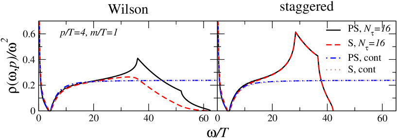
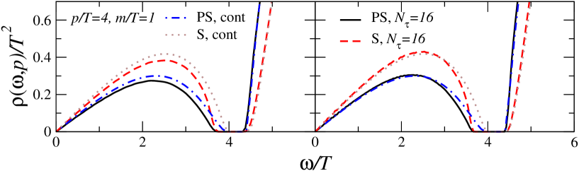
Figure 1: Pseudoscalar and scalar spectral functions $\rho_{\rm PS,S}(\omega,{\mathbf{p}})/\omega^{2}$ (above) and $\rho_{\rm PS,S}(\omega,{\mathbf{p}})/T^{2}$ (below) as a function of $\omega/T$ for $N_{\tau}=16$, $p/T=4,m/T=1$ and $\xi=1$.

In Fig. 1 we show the scalar and pseudoscalar spectral functions for Wilson (left) and staggered (right) fermions. In order to emphasize the effects of the lattice cutoff, $\rho_{\rm PS,S}$ is divided by $\omega^{2}$ in the top figures. The continuum result then reaches a constant value ($3/4\pi$) for large $\omega$, see Eq. (13). Instead, on the lattice there is a maximal energy $\omega_{\rm max}$, determined by the delta function $\delta(\omega-E_{\mathbf{k}}-E_{\mathbf{r}})$. Since the external momentum ${\mathbf{p}}$ is small with respect to momenta at the edge of the Brillouin zone, the maximum value for Wilson fermions (with $r=1$) is determined by fermion momenta ${\mathbf{k}}=(\pi/a,\pi/a,\pi/a)$ [10], which gives

$$\frac{\omega_{\rm max}^{\rm Wilson}}{T}\approx 2N_{\tau}\ln\left(1+\frac{6+am}{\xi}\right),$$ (52)

and for staggered fermions by fermion momenta ${\mathbf{k}}=(\pi/2a,\pi/2a,\pi/2a)$, which yields

$$\frac{\omega_{\rm max}^{\rm naive}}{T}\approx 2N_{\tau}\ln\frac{\sqrt{\xi^{2}+3+a^{2}m^{2}}+\sqrt{3+a^{2}m^{2}}}{\xi}.$$ (53)

The maximum value is smaller for staggered fermions. The cusps in the plots originate from the corners of the Brillouin zone. Both for continuum and staggered fermions, we find that the scalar and pseudoscalar channel are indistinguishable for large $\omega$. The reason is that the finite fermion mass is negligible for such large energies. In the case of Wilson fermions the Wilson mass term breaks the chiral symmetry completely and the scalar and pseudoscalar spectral functions differ.

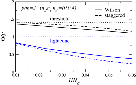
Figure 2: Effect of finite lattice spacing on the ’lightcone’ and ’threshold’ for fixed $pL\approx 25$ and $m=p/2$. The continuum values are $\omega/p=1$ resp. $\omega/p=\sqrt{1+4m^{2}/p^{2}}=\sqrt{2}$.

The spectral functions vanish for energies $p<\omega<\sqrt{p^{2}+4m^{2}}$. The physically interesting contribution below the lightcone appears as a divergent one in the top plots. We therefore show $\rho_{\rm PS,S}/T^{2}$ in the plots on the bottom. The spectral functions increase linearly for small $\omega$ and vanish at the lightcone. Due the finite fermion mass, the scalar and the pseudoscalar channel are now physically distinct. The main lattice artefact in this region appears to be the mismatch between the location of the lightcone in the continuum and the lattice theory. This is due to the difference between continuum and lattice dispersion relations. To study this further, we define the lattice ’lightcone’ and ’threshold’ via

$$\mbox{lightcone:}\;\;\;\omega=\max_{\mathbf{k}}(E_{\mathbf{k}}-E_{{\mathbf{k}}+{\mathbf{p}}}),\;\;\;\;\;\;\;\;\;\mbox{threshold:}\;\;\;\omega=\min_{\mathbf{k}}(E_{\mathbf{k}}+E_{{\mathbf{k}}+{\mathbf{p}}}).$$ (54)

In Fig. 2 we show the result as a function of $1/N_{\sigma}\sim a$ for fixed momentum ${\mathbf{p}}=(0,0,8\pi/aN_{\sigma})$ ($pL\approx 25$) and $m=p/2$. As expected, the continuum and lattice results agree for decreasing $1/N_{\sigma}$ (decreasing lattice spacing), but for finite $a$ the corrections can be substantial.

     

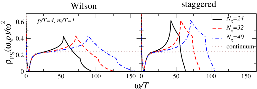
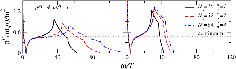
Figure 3: Pseudoscalar spectral functions $\rho_{\rm PS}(\omega,{\mathbf{p}})/\omega^{2}$ as a function of $\omega/T$ for $N_{\tau}=24,32,40$ and $\xi=1$ (above) and vector spectral functions $\rho^{ii}(\omega,{\mathbf{p}})/\omega^{2}$ as a function of $\omega/T$ for $(N_{\tau},\xi)=(16,1),(32,2),(64,4)$ (below). In both cases $p/T=4,m/T=1$.

The effect of increasing $N_{\tau}$ is demonstrated in Fig. 3 for the pseudoscalar spectral function $\rho_{\rm PS}$ for fixed $\xi=1$ (top) and for the vector spectral function $\rho^{ii}$ for fixed $\xi/N_{\tau}=aT$ (bottom). As expected from Eqs. (52) and (53), $\omega_{\rm max}$ increases with $N_{\tau}$. In the anisotropic case, a large $N_{\tau}$ seems to lead to a better improvement for Wilson than for staggered fermions. In Fig. 4, we present our results for $\rho^{00}$. As we emphasized in Eq. (14), due to current conservation this spectral function does not increase with $\omega^{2}$ for large $\omega$, but instead reaches a constant value $p^{2}/2\pi$. This can indeed be seen in Fig. 4. Due to this behaviour the contribution below the lightcone is visible in the same plot. In this case it appears that staggered fermions reproduce the continuum result substantially better than Wilson fermions.

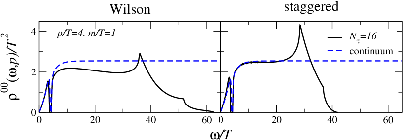
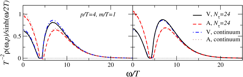
Figure 4: Spectral functions $\rho^{00}(\omega,{\mathbf{p}})/T^{2}$ as a function of $\omega/T$ for $N_{\tau}=16$ (above). Spectral functions $\rho_{\rm V,A}(\omega,{\mathbf{p}})/T^{2}\sinh(\omega/2T)$ as a function of $\omega/T$ for $N_{\tau}=24$ (below). In both cases $p/T=4,m/T=1$ and $\xi=1$.

Finally, we note that the following behaviour of the kernel and spectral functions ($\rho^{00}$ and $\rho^{00}_{5}$ excluded)

$$\omega\to 0: \;\;\;\;\;\;\rho_{H}(\omega,{\mathbf{p}})\approx\omega,\;\;\;\;\;\;\;K(\tau,\omega)\approx\frac{2T}{\omega},$$

$$\omega\to\infty: \;\;\;\;\;\;\rho_{H}(\omega,{\mathbf{p}})\approx\omega^{2},\;\;\;\;\;\;K(\tau,\omega)\approx e^{-\omega\tau}+e^{\omega(\tau-1/T)},$$ (55)

makes it difficult to study spectral functions for both small and large energies in one plot. This can be circumvented by instead showing the integrand at the midpoint $\tau=1/2T$, i.e.,

$$K(1/2T,\omega)\rho_{H}(\omega,{\mathbf{p}})=\frac{\rho_{H}(\omega,{\mathbf{p}})}{\sinh(\omega/2T)},$$ (56)

which takes a finite value for $\omega\to 0$ and vanishes exponentially for large $\omega$. In Fig. 4 we show an example of this for $\rho_{\rm V,A}$. Since the region with large $\omega$ is exponentially suppressed, we note that the lattice artefacts related to the finiteness of the Brillioun zone discussed above give an exponentially small contribution. We conclude therefore that the euclidean correlator at the midpoint $G_{H}(1/2T,{\mathbf{p}})$ is largely insensitive to these artefacts. We also point out that it follows from the analysis in Section 3.3 that the area under the curves are identical: the larger spectral weight of $\rho_{\rm A}$ below the lightcone is exactly compensated by the larger spectral weight of $\rho_{\rm V}$ above threshold.

5 Summary

We have studied meson spectral functions at nonzero momentum in the infinite temperature limit, in the continuum and on the lattice using Wilson and staggered fermions. We found that for large values of the energy $\omega$, lattice spectral functions become sensitive to the effects of discretizaton and deviate from the continuum expectation, in agreement with the conclusions from Ref. [10]. For smaller $\omega$, finite discretization affects predominantly the mismatch between the continuum and lattice lightcone, which can be substantial. In the free field limit a simple relationship between the euclidean correlators in different channels at the midpoint was found.

A qualitative comparison between the results obtained with staggered and Wilson fermions suggests that in the low-energy region lattice artefacts are less prominent for the staggered formulation. The use of an anisotropic lattice, on the other hand, seems to be more beneficial for Wilson fermions.

Acknowledgments. It is a pleasure to thank Simon Hands and Seyong Kim for numerous discussions. J.M.M.R. thanks the Physics Department in Swansea for its hospitality during the course of this work. G.A. is supported by a PPARC Advanced Fellowship. J.M.M.R. was supported in part by the Spanish Science Ministry (Grant FPA 2002-02037) and the University of the Basque Country (Grant UPV00172.310-14497/2002).

References

- [1] M. Asakawa, T. Hatsuda and Y. Nakahara, Prog. Part. Nucl. Phys. 46, 459 (2001) [hep-lat/0011040].
- [2] M. Asakawa and T. Hatsuda, Phys. Rev. Lett. 92, 012001 (2004) [hep-lat/0308034].
- [3] S. Datta, F. Karsch, P. Petreczky and I. Wetzorke, Phys. Rev. D 69, 094507 (2004) [hep-lat/0312037].
- [4] T. Umeda, K. Nomura and H. Matsufuru, Eur. Phys. J. C 39S1, 9 (2005) [hep-lat/0211003].
- [5] F. Karsch, E. Laermann, P. Petreczky, S. Stickan and I. Wetzorke, Phys. Lett. B 530, 147 (2002) [hep-lat/0110208].
- [6] S. Gupta, Phys. Lett. B 597, 57 (2004) [hep-lat/0301006].
- [7] A. Nakamura and S. Sakai, Phys. Rev. Lett. 94, 072305 (2005) [hep-lat/0406009].
- [8] F. Karsch and H. W. Wyld, Phys. Rev. D 35, 2518 (1987).
- [9] G. Aarts and J. M. Martínez Resco, JHEP 0204 (2002) 053 [hep-ph/0203177]; Nucl. Phys. Proc. Suppl. 119 (2003) 505 [hep-lat/0209033].
- [10] F. Karsch, E. Laermann, P. Petreczky and S. Stickan, Phys. Rev. D 68, 014504 (2003) [hep-lat/0303017].
- [11] E. Braaten and R. D. Pisarski, Nucl. Phys. B 337, 569 (1990).
- [12] E. Braaten, R. D. Pisarski and T. C. Yuan, Phys. Rev. Lett. 64, 2242 (1990).
- [13] F. Karsch, M. G. Mustafa and M. H. Thoma, Phys. Lett. B 497, 249 (2001) [hep-ph/0007093].
- [14] W. M. Alberico, A. Beraudo and A. Molinari, Nucl. Phys. A 750, 359 (2005) [hep-ph/0411346].
- [15] P. Aurenche, F. Gelis, R. Kobes and H. Zaraket, Phys. Rev. D 58, 085003 (1998) [hep-ph/9804224].
- [16] P. Arnold, G. D. Moore and L. G. Yaffe, JHEP 0112, 009 (2001) [hep-ph/0111107].
- [17] P. Aurenche, F. Gelis, G. D. Moore and H. Zaraket, JHEP 0212, 006 (2002) [hep-ph/0211036].
- [18] L. P. Kadanoff and P. C. Martin, Ann. Phys. 24, 419 (1963), reprinted as Ann. Phys. 281, 800 (2000).
- [19] M. A. Valle Basagoiti, Phys. Rev. D 66, 045005 (2002) [hep-ph/0204334].
- [20] G. Aarts and J. M. Martínez Resco, JHEP 0211, 022 (2002) [hep-ph/0209048].
- [21] G. Aarts and J. M. Martínez Resco, JHEP 0503, 074 (2005) [hep-ph/0503161].
- [22] D. B. Carpenter and C. F. Baillie, Nucl. Phys. B 260 (1985) 103.
- [23] N. Kawamoto and J. Smit, Nucl. Phys. B 192, 100 (1981).
- [24] L. H. Karsten and J. Smit, Nucl. Phys. B 183, 103 (1981).