DESY/05-090 SFB/CPP-05-20 June 2005
HMC algorithm with multiple time scale
integration and mass preconditioning

We present a variant of the HMC algorithm with mass preconditioning (Hasenbusch acceleration) and multiple time scale integration. We have tested this variant for standard Wilson fermions at $\beta=5.6$ and at pion masses ranging from $380$MeV to $680$MeV. We show that in this situation its performance is comparable to the recently proposed HMC variant with domain decomposition as preconditioner. We give an update of the “Berlin Wall” figure, comparing the performance of our variant of the HMC algorithm to other published performance data. Advantages of the HMC algorithm with mass preconditioning and multiple time scale integration are that it is straightforward to implement and can be used in combination with a wide variety of lattice Dirac operators.

1 Introduction

Simulations of full QCD with light dynamical flavors of quarks and at small lattice spacing are presently one of the greatest challenges in lattice QCD. Simulations in this regime have to face the phenomenon of critical slowing down: in addition to the “natural” increase of costs due to increasing volume and increasing iteration numbers needed in the solvers, the autocorrelation times are expected to grow significantly when the masses are decreased.

One widely used algorithm to perform those simulations is the Hybrid Monte Carlo (HMC) algorithm [1], an exact algorithm which combines molecular dynamics evolution of the gauge fields with a Metropolis accept/reject step to correct for discretization errors in the numerical integration of the corresponding equations of motion. However, in its original form the HMC algorithm is even on nowadays computers not able to tackle simulations with light quarks on fine lattices, for the reasons stated above.

Therefore a lot of effort has been invested to accelerate the HMC algorithm during the last years and the corresponding list of improvements that were found is long. It reaches, for example, from even/odd preconditioning [2] over multiple time scale integration [3] and chronological inversion methods [4] to mass preconditioning (Hasenbusch acceleration) [5, 6], to mention only those that are immediately relevant for the present paper. It is worth noting that many of the known improvement tricks can be combined. In addition, alternative multiboson methods [7] have been suggested, which, however, appear not to be superior to the HMC algorithm.

Recently in ref. [8] a HMC variant as a combination of multiple time scale integration with domain decomposition as preconditioner on top of even/odd preconditioning was presented and speedup factors of about $10$ were reported when compared to state of the art simulations using a HMC algorithm [9]. Even more important, excellent scaling properties with the quark mass were found. Thus this algorithm seems to be most promising when one wants to simulate small quark masses on fine lattices.

In this paper we are going to present yet another variant of the HMC algorithm similar to the one of refs. [10, 11] comprising multiple time scale integration with mass preconditioning on top of even/odd preconditioning. We test this algorithm for standard Wilson fermions at $\beta=5.6$ and at pion masses ranging from $m_{\pi}=370$MeV to $m_{\pi}=650$MeV. We show that in this situation the algorithm has similar scaling properties and performance as the method presented in ref. [8]. From the performance data obtained with our HMC variant we update the “Berlin Wall” figures of refs. [12, 13] and find that the picture is significantly improved.

After shortly recalling the HMC algorithm as well as the ideas of multiple time scale integration and mass preconditioning, we will present numerical results comparing our HMC version with the one of refs. [8, 9] and draw our conclusions.

2 HMC algorithm

The variant of the HMC algorithm we will present here is applicable to a wide class of lattice Dirac operators, including twisted mass fermions, various improved versions of Wilson fermions, staggered fermions, and even the overlap operator. Nevertheless, in order to discuss a concrete example, we restrict ourselves in this paper to the Wilson-Dirac operator with Wilson parameter $r$ set to one

$$D_{\mathrm{W}}[U,m_{0}]=\frac{1}{2}\sum_{\mu}\left\{(\nabla_{\mu}+\nabla_{\mu}^{*})\gamma_{\mu}-a\nabla_{\mu}^{*}\nabla_{\mu}\right\}+m_{0}\,,$$ (2-1)

where $m_{0}$ is the bare mass parameter, and $\nabla_{\mu}$ and $\nabla_{\mu}^{*}$ the gauge covariant lattice forward and backward difference operators, respectively. The Wilson lattice action can be written as

$$S[U,m_{0}]=S_{\mathrm{G}}[U]+a^{4}\sum_{x}\bar{\psi}(x)\left(D_{\mathrm{W}}[U,m_{0}]\right)\psi(x)\,,$$ (2-2)

where $S_{\mathrm{G}}[U]$ is the usual Wilson plaquette gauge action. In the implementation we use the so-called hopping parameter representation of eq. (2-2), where the hopping parameter is defined to be

$$\kappa=(2m_{0}+8)^{-1}\,,$$

and the fermion fields are rescaled according to

$$\psi\ \to\ \frac{\sqrt{2\kappa}}{a^{3/2}}\psi\,,\qquad\bar{\psi}\ \to\ \frac{\sqrt{2\kappa}}{a^{3/2}}\bar{\psi}\,.$$

After integrating out the fermion fields $\psi,\bar{\psi}$ the partition function of lattice QCD for $n_{f}=2$ mass degenerate flavors of quarks reads

$$\mathcal{Z}=\int\mathcal{D}U\det(D_{\mathrm{W}}[U,m_{0}])^{2}e^{-S_{\mathrm{G}}[U]}\ .$$ (2-3)

Since $D_{\mathrm{W}}$ fulfills the property $\gamma_{5}D_{\mathrm{W}}\gamma_{5}=D_{\mathrm{W}}^{\dagger}$ we define for later purpose the hermitian Wilson-Dirac operator

$$Q=\gamma_{5}D_{\mathrm{W}}\,.$$ (2-4)

In order to prepare the set up for the Hybrid Monte Carlo (HMC) algorithm [1], the determinant $\det(D_{\mathrm{W}}[U,m_{0}])$ is usually re-expressed by the use of so-called pseudo fermion fields $\phi$

$$\det(D_{\mathrm{W}})^{2}=\det(Q)^{2}\propto\int\mathcal{D}\phi^{\dagger}\mathcal{D}\phi\exp\Bigl{(}-S_{\mathrm{PF}}[U,\phi^{\dagger},\phi]\Bigr{)}\,,$$ (2-5)

where $S_{\mathrm{PF}}[U,\phi^{\dagger},\phi]=|Q^{-1}\phi|^{2}$ is the pseudo fermion action. The pseudo fermion fields $\phi$ are formally identical to the fermion fields $\psi$, but follow the statistic of bosonic fields. The $\phi$ version of the HMC algorithm is based on the Hamiltonian

$$H(P,U,\phi,\phi^{\dagger})=\frac{1}{2}\sum_{x,\mu}P_{x,\mu}^{2}+S_{\mathrm{G}}[U]+S_{\mathrm{PF}}[U,\phi,\phi^{\dagger}]\,,$$ (2-6)

where we introduced traceless Hermitian momenta $P_{x,\mu}$ as conjugate fields to the gauge fields $U_{x,\mu}$. The HMC algorithm is then composed out of molecular dynamics evolution of the gauge fields and momenta and a Metropolis accept/reject step, which is needed to correct for the discretization errors of the numerical integration of the corresponding equations of motion.

It is possible to prove that the HMC algorithm satisfies the detailed balance condition [1] and hence the configurations generated with this algorithm correctly represent the intended ensemble.

2.1 Molecular dynamics evolution

In the molecular dynamics part of the HMC algorithm the gauge fields $U$ and the momenta $P$ need to be evolved in a fictitious computer time $t$. With respect to $t$, Hamilton’s equations of motion read

$$\frac{dU}{dt}=\frac{dH}{dP}=P\,,\qquad\frac{dP}{dt}=-\frac{dH}{dU}=-\frac{dS}{dU}\,,$$ (2-7)

where we set $S=S_{\mathrm{G}}+S_{\mathrm{PF}}$ and $d/dU$, $d/dP$ formally denote the derivative with respect to group elements. Since analytical integration of the former equations of motion is normally not possible, these equations must in general be integrated with a discretized integration scheme that is area preserving and reversible, such as the leap frog algorithm. The discrete update with integration step size $\Delta\tau$ of the gauge field and the momenta can be defined as

$$\begin{split}T_{\mathrm{U}}(\Delta\tau)&:\quad U\quad\to\quad U^{\prime}=\exp\left(i\Delta\tau P\right)U\,,\\ T_{\mathrm{S}}(\Delta\tau)&:\quad P\quad\to\quad P^{\prime}=P-i\Delta\tau\delta S\,,\\ \end{split}$$ (2-8)

where $\delta S$ is an element of the Lie algebra of $\mathrm{SU}(3)$ and denotes the variation of $S$ with respect to the gauge fields. The computation of $\delta S$ is the most expensive part in the HMC algorithm since the inversion of the Wilson-Dirac operator is needed. With (2-8) one basic time evolution step of the so called leap frog algorithm reads

$$T=T_{\mathrm{S}}(\Delta\tau/2)\ T_{\mathrm{U}}(\Delta\tau)\ T_{\mathrm{S}}(\Delta\tau/2)\,,$$ (2-9)

and a whole trajectory of length $\tau$ is achieved by $N_{\mathrm{MD}}=\tau/\Delta\tau$ successive applications of the transformation $T$.

2.2 Integration with multiple time scales

In order to generalize the leap frog integration scheme we assume in the following that we can bring the Hamiltonian to the form

$$H=\frac{1}{2}\sum_{x,\mu}P_{x,\mu}^{2}+\sum_{i=0}^{k}S_{i}[U]\,,$$ (2-10)

with $k\geq 1$. For instance with $k=1$ $S_{0}$ might be identified with the gauge action and $S_{1}$ with the pseudo fermion action of eq. (2-6).

Given a form of the Hamiltonian (2-10) one can think of the following situations in which it might be favorable to use a generalized leap frog integration scheme where the different parts $S_{i}$ are integrated with different step sizes, as proposed in ref. [3].

Clearly, in order to keep the discretization errors in a leap frog like algorithm small, the time steps have to be small if the driving forces are large. Hence multiple time scale integration is a valuable tool if the forces originating from the single parts in the Hamiltonian (2-10) differ significantly in their absolute values. Then the different parts in the Hamiltonian might be integrated on time scales inverse proportionally deduced from the corresponding forces.

Another situation in which multiple time scales might be useful exists when one part in the Hamiltonian (2-10) is significantly cheaper to update than the others. In this case the cheap part might be integrated without too much performance loss on a smaller time scale, which reduces the discretization errors coming from that part.

The leap frog integration scheme can be generalized to multiple time scales as has been proposed in ref. [3] without loss of reversibility and the area preserving property. The scheme with only one time scale can be recursively extended by starting with the definition

$$T_{0}=T_{\mathrm{S}_{0}}(\Delta\tau_{0}/2)\ T_{\mathrm{U}}(\Delta\tau_{0})\ T_{\mathrm{S}_{0}}(\Delta\tau_{0}/2)\,,$$ (2-11)

with $T_{\mathrm{U}}$ defined as in eq. (2-8) and where $T_{\mathrm{S}_{i}}(\Delta\tau)$ is given by

$$T_{\mathrm{S}_{i}}(\Delta\tau)\quad:\quad P\quad\to\quad P-i\Delta\tau\delta S_{i}[U]\,.$$ (2-12)

As $\Delta\tau_{0}$ will be the smallest time scale, we can recursively define the basic update steps $T_{i}$, with time scales $\Delta\tau_{i}$ as

$$T_{i}=T_{\mathrm{S}_{i}}(\Delta\tau_{i}/2)\ [T_{i-1}]^{N_{i-1}}\ T_{\mathrm{S}_{i}}(\Delta\tau_{i}/2)\,,$$ (2-13)

with integers $N_{i}$ and $0<i\leq k$. One full trajectory $\tau$ is then composed by $[T_{k}]^{N_{k}}$. The different time scales $\Delta\tau_{i}$ in eq. (2-13) must be chosen such that the total number of steps on the $i$-th time scale $N_{\mathrm{MD}_{i}}$ times $\Delta\tau_{i}$ is equal to the trajectory length $\tau$ for all $0\leq i\leq k$: $N_{\mathrm{MD}_{i}}\Delta\tau_{i}=\tau$. This is obviously achieved by setting

$$\Delta\tau_{i}=\frac{\tau}{N_{k}\cdot N_{k-1}\cdot...\cdot N_{i}}=\frac{\tau}{N_{\mathrm{MD}_{i}}}\,,\qquad 0\leq i\leq k\,,$$ (2-14)

where $N_{\mathrm{MD}_{i}}=N_{k}\cdot N_{k-1}\cdot...\cdot N_{i}$.

In ref. [3] also a partially improved integration scheme with multiple time scales was introduced, which reduces the size of the discretization errors. Again, we assume a Hamiltonian of the form (2-10) with now $k=1$. By defining similar to $T_{0}$

$$T_{\mathrm{SW}_{0}}\ =\ T_{\mathrm{S}_{0}}(\Delta\tau_{0}/6)\ T_{\mathrm{U}}(\Delta\tau_{0}/2)\ T_{\mathrm{S}_{0}}(2\Delta\tau_{0}/3)\ T_{\mathrm{U}}(\Delta\tau_{0}/2)\ T_{\mathrm{S}_{0}}(\Delta\tau_{0}/6)\,,$$ (2-15)

the basic update step of the improved scheme – usually referred to as the Sexton-Weingarten (SW) integration scheme – reads

$$\begin{split}T_{\mathrm{SW}_{1}}=&T_{\mathrm{S}_{1}}(\Delta\tau_{1}/6)\\ &[T_{\mathrm{SW}_{0}}]^{N_{0}}\ T_{\mathrm{S}_{1}}(2\Delta\tau_{1}/3)\\ &[T_{\mathrm{SW}_{0}}]^{N_{0}}\ T_{\mathrm{S}_{1}}(\Delta\tau_{1}/6)\,,\end{split}$$ (2-16)

where $\Delta\tau_{0}=\Delta\tau_{1}/(2N_{0})$. This integration scheme not only reduces the size of the discretization errors, but also sets for $S_{0}$ a different time scale than for $S_{1}$. Hence, it is one special example for an integration scheme with multiple time scales and can easily be extended to more than two time scales by recursively defining ($0<i\leq k$):

$$\begin{split}T_{\mathrm{SW}_{i}}=&T_{S_{i}}(\Delta\tau_{i}/6)\ \\ &[T_{\mathrm{SW}_{i-1}}]^{N_{i-1}}\ T_{S_{i}}(2\Delta\tau_{i}/3)\\ &[T_{\mathrm{SW}_{i-1}}]^{N_{i-1}}\ T_{S_{i}}(\Delta\tau_{i}/6)\,.\end{split}$$ (2-17)

The different time scales for the SW integration scheme are defined by

$$\Delta\tau_{i}=\frac{\tau}{(2N_{k})\cdot(2N_{k-1})\cdot...\cdot(2N_{i})}=\frac{\tau}{N_{\mathrm{MD}_{i}}}\,,\qquad i\leq k\,.$$ (2-18)

Note that the SW partially improved integration scheme makes use of the fact that the computation of the variation of the gauge action is cheap compared to the variation of the pseudo fermion action and in addition the time scales are chosen in order to cancel certain terms in the discretization error exactly.

3 Mass Preconditioning

The arguments presented in this section are made for simplicity only for the not even/odd preconditioned Wilson-Dirac operator. The generalization to the even/odd preconditioned case is simple and can be found in ref. [5] and the appendix of ref. [14].

Mass preconditioning [5] – also known as Hasenbusch acceleration – relies on the observation that one can rewrite the fermion determinant as follows

$$\begin{split}\det(Q^{2})&=\det(W^{+}W^{-})\frac{\det(Q^{2})}{\det(W^{+}W^{-})}\\ &=\int\mathcal{D}\phi_{1}^{\dagger}\mathcal{D}\phi_{1}\ \mathcal{D}\phi_{2}^{\dagger}\mathcal{D}\phi_{2}\ e^{-\phi_{1}^{\dagger}\frac{1}{W^{+}W^{-}}\phi_{1}-\phi_{2}^{\dagger}W^{+}\frac{1}{Q^{2}}W^{-}\phi_{2}}\\ &=\int\mathcal{D}\phi_{1}^{\dagger}\mathcal{D}\phi_{1}\ \mathcal{D}\phi_{2}^{\dagger}\mathcal{D}\phi_{2}\ e^{-S_{\textrm{PF}_{1}}-S_{\textrm{PF}_{2}}}\,.\end{split}$$ (3-1)

The preconditioning operators $W^{\pm}$ can in principle be freely chosen, but in order to let the preconditioning work $W^{+}W^{-}$ should be a reasonable approximation of $Q^{2}$, which is, however, cheaper to simulate. Moreover, to allow for Monte Carlo simulations, $\det(W^{+}W^{-})$ must be positive. The generalized Hamiltonian (2-6) corresponding to eq. (3-1) reads

$$H=\frac{1}{2}\sum_{x,\mu}P_{x,\mu}^{2}+S_{\textrm{G}}[U]+S_{\textrm{PF}_{1}}[U,\phi_{1},\phi_{1}^{\dagger}]+S_{\textrm{PF}_{2}}[U,\phi_{2},\phi_{2}^{\dagger}]\,,$$ (3-2)

and it can of course be extended to more than one additional field.

Note that a similar approach was presented in ref. [15], in which the introduction of $n$ pseudo fermion fields was coupled with the $n$-th root of the fermionic kernel.

One particular choice for $W^{\pm}$ is given by

$$W^{\pm}=Q\pm i\mu\,,$$ (3-3)

with mass parameter $\mu$ refered to as a twisted mass parameter. In fact the operator

$$\begin{pmatrix}W^{+}&\\ &W^{-}\\ \end{pmatrix}=\begin{pmatrix}Q&\\ &Q\\ \end{pmatrix}+i\mu\tau_{3}$$ (3-4)

is the two flavor twisted mass operator with $\tau_{3}$ the third Pauli matrix acting in flavor space. One important property of this choice is that $W^{+}W^{-}=Q^{2}+\mu^{2}$. Note that $(W^{+})^{\dagger}=W^{-}$ and we remark that in general also $Q$ can be a twisted mass operator.

In ref. [6, 16] it was argued that the optimal choice for $\mu$ is given by $\mu^{2}=\sqrt{\lambda_{\mathrm{max}}\lambda_{\mathrm{min}}}$. Here $\lambda_{\mathrm{max}}$ ($\lambda_{\mathrm{min}}$) is the maximal (minimal) eigenvalue of $Q^{2}$. The reason for the above quoted choice is as follows: the condition number of $Q^{2}+\mu^{2}$ is approximately $\lambda_{\mathrm{max}}/\mu^{2}$ and the one of $Q^{2}/(Q^{2}+\mu^{2})$ approximately $\mu^{2}/\lambda_{\mathrm{min}}$. With $\mu^{2}=\sqrt{\lambda_{\mathrm{max}}\lambda_{\mathrm{min}}}$ these two condition numbers are equal to $\sqrt{\lambda_{\mathrm{max}}/\lambda_{\mathrm{min}}}$, both of them being much smaller than the condition number of $Q^{2}$ which is $\lambda_{\mathrm{max}}/\lambda_{\mathrm{min}}$.

Since the force contribution in the molecular dynamics evolution is supposed to be proportional to some power of the condition number, the force contribution from the pseudo fermion part in the action is reduced and therefore the step size $\Delta\tau$ can be increased, in practice by about a factor of $2$ [5, 6]. Therefore $Q^{2}$ must be inverted only about half as often as before and if the inversion of $W^{+}W^{-}$, which is needed to compute $\delta S_{\mathrm{PF}_{1}}$, is cheap compared to the one of $Q^{2}$ the simulation speeds up by about a factor of two [5, 6].

One might wonder why the reduction of the condition number from $K$ to $\sqrt{K}$ gives rise to only a speedup factor of about $2$. One reason for this is that one cannot make use of the reduced condition number of $Q^{2}/(Q^{2}+\mu^{2})$ in the inversion of this operator, because in the actual simulation still the badly conditioned operator $Q^{2}$ must be inverted to compute the variation of $S_{\textrm{PF}_{2}}=\phi_{2}^{\dagger}\frac{W^{+}W^{-}}{Q^{2}}\phi_{2}$.

3.1 Mass preconditioning and multiple time scale integration

In the last subsection we have seen that mass preconditioning is indeed an effective tool to change the condition numbers of the single operators appearing in the factorization (3-1) compared to the original operator. But, this reduction of the condition numbers only influences the forces – which are proportional to some power of the condition numbers of the corresponding operators – and not the number of iterations to invert the physical operator $Q^{2}$.

Therefore it might be advantageous to change the point of view: instead of tuning the condition numbers in a way à la refs. [5, 6] we will exploit the possibility of arranging the forces by the help of mass preconditioning with the aim to arrange for a situation in which a multiple time scale integration scheme is favorable, as explained at the beginning of subsection 2.2.

The procedure can be summarized as follows: use mass preconditioning to split the Hamiltonian in different parts. The forces of the single parts should be adjusted by tuning the preconditioning mass parameter $\mu$ such that the more expensive the computation of $\delta S_{\mathrm{PF}_{i}}$ is, the less it contributes to the total force. This is possible because the variation of $(Q^{2}+\mu^{2})/Q^{2}$ is, for $|\mu|<1$, reduced by a factor $\mu^{2}$ compared to the variation of $1/Q^{2}$. In addition, $W^{+}W^{-}=Q^{2}+\mu^{2}$ is significantly cheaper to invert than $Q^{2}$. Then integrate the different parts on time scales chosen according to the magnitude of their force contribution.

The idea presented in this paper is very similar to the idea of separating infrared and ultraviolet modes as proposed in ref. [17]. This idea was applied to mass preconditioning by using only two time scales in refs. [10, 11] in the context of clover improved Wilson fermions. However, a comparison of our results presented in the next section to the ones of refs. [10, 11] is not possible, because volume, lattice spacing and masses are different.

4 Numerical results

4.1 Simulation points

In order to test the HMC variant introduced in the last sections, we decided to compare it with the algorithm proposed and tested in ref. [8]. To this end we performed simulations with the same parameters as have been used in ref. [8]: Wilson-Dirac operator with plaquette gauge action at $\beta=5.6$ on $24^{3}\times 32$ lattices. We have three simulation points $A$, $B$ and $C$ with values of the hopping parameter $\kappa=0.1575$, $\kappa=0.1580$ and $\kappa=0.15825$, respectively. The trajectory length was set to $\tau=0.5$. The details of the physical parameters corresponding to the different simulation points can be found in table 1. Additionally, this choice of simulation points allows at the two parameter sets $A$ and $B$ a comparison to results published in ref. [9], where a HMC algorithm with a plain leap frog integration scheme was used.

$\Bigl{.}\Bigr{.}$	$\kappa$	$m_{q}/\mathrm{MeV}$	$m_{\mathrm{PS}}/\mathrm{MeV}$	$m_{\mathrm{V}}/\mathrm{MeV}$	$r_{0}/a$
$\Bigl{.}\Bigr{.}A$	$0.1575$	$66(3)$	$665(17)$	$947(20)$	$6.04(10)$
$\Bigl{.}\Bigr{.}B$	$0.1580$	$34(1)$	$485(13)$	$836(24)$	$6.18(07)$
$\Bigl{.}\Bigr{.}C$	$0.15825$	$22(1)$	$380(17)$	$839(33)$	$6.40(15)$

Table 1: The (unrenormalized) quark mass $m_{q}$, the pseudo scalar mass $m_{\mathrm{PS}}$ and the vector mass $m_{\mathrm{V}}$ are given in in physical units at the three simulation points $A$, $B$ and $C$. We use Wilson fermions at $\beta=5.6$ on $24^{3}\times 32$ lattices. The scale was set by the use of $r_{0}=0.5\,\mathrm{fm}$ and we give the value of $r_{0}/a$ at each simulation point. The values of all the quantities agree within the errors with the numbers quoted in refs. [8, 18, 9], apart from the value for $r_{0}/a$ at simulation point $B$, which disagrees by two sigmas to the value quoted in ref. [18]. This is presumably due to the different methods to measure this quantity. For the measurements we used at each simulation point $100$ thermalized configurations separated by $5$ trajectories.

4.2 Details of the implementation

We have implemented a HMC algorithm for two flavors of mass degenerate quarks with even/odd preconditioning and mass preconditioning with up to three pseudo fermion fields. The boundary conditions are periodic in all directions apart from anti-periodic ones for the fermion fields in time direction. For details of the implementation see the appendix of ref. [14]. For the gauge action the usual Wilson plaquette gauge action is used. The implementation is written in C and uses double precision throughout.

For the mass preconditioning we use

$$W^{\pm}_{j}=\gamma_{5}(D_{\mathrm{W}}[U,m_{0}]\pm i\mu_{j}\gamma_{5})\,,$$ (4-1)

with $j=1,2$ for the factorization in eq. (3-1), where the $\mu_{j}$ are the additional (unphysical) twisted mass parameters. Therefore, the pseudo fermion actions $S_{\textrm{PF}_{j}}$ are given by

$$S_{\textrm{PF}_{j}}[U]=\begin{cases}\biggl{.}\phi_{1}^{\dagger}\left(\frac{1}{W^{+}_{1}W^{-}_{1}}\right)\phi_{1}&j=1\,\biggr{.},\\ \biggl{.}\phi_{j}^{\dagger}\left(\frac{W^{+}_{j-1}W^{-}_{j-1}}{Q^{2}}\right)\phi_{j}&j=N_{\mathrm{PF}}\biggr{.}\,,\\ \biggl{.}\phi_{j}^{\dagger}\left(\frac{W^{+}_{j-1}W^{-}_{j-1}}{W^{+}_{j}W^{-}_{j}}\right)\phi_{j}\biggr{.}&\text{otherwise}\,,\\ \end{cases}$$ (4-2)

where we always chose $0<\mu_{1}<\mu_{2}$ and $N_{\mathrm{PF}}$ denotes the actually used number of pseudo fermion fields.

We have implemented the leap frog (LF) and the Sexton-Weingarten (SW) integration schemes with multiple time scales each as described by eq. (2-13) and eq. (2-17), respectively, where $k$ in both equations has to be identified with $N_{\mathrm{PF}}$.

The time scales are defined as in eq. (2-14) for the LF integration scheme and as in eq. (2-18) for the SW scheme, with $N_{0}$ corresponding to the gauge action and $N_{j}$ to $S_{\mathrm{PF}_{j}}$ for $N_{\mathrm{PF}}\geq j>0$. Note that for the LF integration scheme for one trajectory there are $N_{N_{\mathrm{PF}}}\cdot\ldots\cdot N_{j}+1$ inversions of the corresponding operator needed, while for the SW integration scheme there are $2N_{N_{\mathrm{PF}}}\cdot\ldots\cdot 2N_{j}+1$ inversions needed.

For the inversions we used the CG and the BiCGstab iterative solvers. We have tested the performance of several iterative solvers for the even/odd preconditioned twisted mass operator [19] with the result, that the CG iterative solver is the best choice in presence of a twisted mass. Thus we used for all inversions of mass preconditioning operators exclusively the CG iterative solver.

For the pure Wilson-Dirac operator $D_{\mathrm{W}}$ the BiCGstab iterative solver is known to perform best [20]. In case of dynamical simulations, however, usually the squared hermitian operator needs to be inverted and in this case the CG is comparable to the BiCGstab. Only in the acceptance step, where $\gamma_{5}D_{\mathrm{W}}$ (or rather the even/odd preconditioned version of it) needs to be inverted to a high precision, the usage of the CG would be wasteful. For this paper we used the BiCGstab iterative solver for all inversions of either the pure Wilson-Dirac operator itself or $(\gamma_{5}D_{\mathrm{W}})^{2}$.

The accuracy in the inversions was set during the computation of $\delta S_{\mathrm{PF}_{j}}$ to $\epsilon_{j}$, which means that the inversions were stopped when the approximate solution $\psi_{j}$ of $A_{j}\psi_{j}=\phi_{j}$ fulfills

$$\frac{\|\phi_{j}-A_{j}\psi_{j}\|}{\|\phi_{j}\|}\leq\epsilon_{j}\,,$$

where $A_{j}$ denotes the operator corresponding to $S_{\mathrm{PF}_{j}}$. During the inversions needed for the acceptance step the accuracy was set to $\tilde{\epsilon}=10^{-10}$ for all pseudo fermion actions. The inversions in the acceptance step must be rather precise in order not to introduce systematic errors in the simulation, while for the force computation the precision can be relaxed as long as the reversibility violations are not too large. The values of $\epsilon_{j}$ and $\tilde{\epsilon}$ have been set such that the reversibility violations, which should be under control [21, 22, 23, 24], are on the same level as reported in ref. [8], which means that the differences in the Hamiltonian are of the order of $10^{-5}$. The values for $\epsilon_{j}$ can be found in table 2.

The errors and autocorrelation times were computed with the so called $\Gamma$-method as explained in ref. [25] (see also ref. [26]), i.e.

$$\tau_{\mathrm{int}}=\frac{1}{2}+\sum_{t=1}^{\infty}\frac{\Gamma(t)}{\Gamma(0)}\,,$$ (4-3)

with the autocorrelation function $\Gamma(t)$.

$\Bigl{.}\Bigr{.}$	Int.	$N_{\mathrm{PF}}$	$N_{\mathrm{therm}}$	$N_{\{\mathrm{0,1,2,3}\}}$	$\epsilon_{1},\epsilon_{2},\epsilon_{3}$	$\mu_{1},\mu_{2}$	$P_{\mathrm{acc}}$
$\Bigl{.}\Bigr{.}A$	SW	$3$	$600$	$3,2,1,3$	$10^{-7},10^{-8},10^{-8}$	$0.29,0.057$	$0.86$
$\Bigl{.}\Bigr{.}B$	SW	$3$	$1000$	$3,2,1,3$	$10^{-8},10^{-8},10^{-8}$	$0.25,0.057$	$0.81$
$\Bigl{.}\Bigr{.}C$	LF	$2$	$1500$	$5,6,10,$ -	$10^{-8},10^{-8},$ -	$0.054,$ -	$0.80$

Table 2: HMC algorithm parameters for the three simulation points. We give the integration scheme, the number of pseudo fermion fields $N_{\mathrm{PF}}$, the number $N_{\mathrm{therm}}$ of trajectories of length $0.5$ used to thermalize the systems, the number $N_{i}$ of molecular dynamics steps for the multiple time scale integration scheme, the residues $\epsilon_{i}$ used in the solver for the force computation, the preconditioning mass parameter $\mu_{i}$ and the acceptance rate. We remind that $N_{0}$ corresponds to the gauge action.

4.3 Force contributions

The force contributions to the total force from the separate parts in the action we label by $F_{G}$ for the gauge action and by $F_{j}$ for the pseudo fermion action $S_{\mathrm{PF}_{j}}$. Since the variation of the action with respect to the gauge fields is an element of the Lie algebra of $\mathrm{SU}(3)$, we used $\|X\|^{2}=-2\operatorname{Tr}{X^{2}}$ as the definition of the norm of such an element.

In order to better understand the influence of mass preconditioning on the HMC algorithm we computed the average and the maximal norm of the forces $F_{G},F_{1},F_{2}$ and $F_{3}$ on a given gauge field after all corresponding gauge field updates:

$$\begin{split}\|F\|_{\mathrm{aver}}&=\frac{1}{4L^{3}T}\sum_{x,\mu}\|F(x,\mu)\|\,,\\ \|F\|_{\mathrm{max}}&=\max_{x,\mu}\{\|F(x,\mu)\|\}\,,\\ \end{split}$$ (4-4)

and averaged them over all measurements, which we indicate with $\langle.\rangle$. Examples of force distributions for different runs can be found in figure 1. These investigations lead to the following observations generic to our simulation points:

• With the choice of parameters as given in table 2 the single force contributions are strictly hierarchically ordered with
  $\|F_{G}\|_{\mathrm{aver,max}}>\|F_{1}\|_{\mathrm{aver,max}}>\|F_{2}\|_{\mathrm{aver,max}}>\|F_{3}\|_{\mathrm{aver,max}}$.

• The maximal force is up to one order of magnitude larger than the average force. This can only be explained by large local fluctuations in this quantity. These fluctuations become larger the smaller the mass is.

Moreover, the force ordering and sizes look very similar to the one reported in ref. [8].

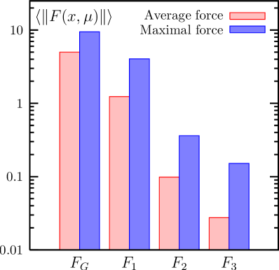
(a) Forces for run $B$.

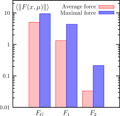
(b) Forces for run $C$.

Figure 1: Average and maximal forces for simulation points $B$ and $C$. The statistical errors are too small to be visible due to the large number of measurements.

In a next step we performed some test trajectories without mass preconditioning in order to compare the fermionic forces with and without mass preconditioning. For the value of $\kappa=0.15825$ (run $C$) the result can be found in figure 2. The bars labeled with $F$ correspond to the fermion force without mass preconditioning. The labels $F_{1}$ and $F_{2}$ refer to the two fermionic forces for the run $C$ with mass preconditioning. The following ratios are of interest:

$$\begin{split}&\frac{\|F\|_{\mathrm{aver}}}{\|F_{1}\|_{\mathrm{aver}}}\approx 1\,,\qquad\frac{\|F\|_{\mathrm{aver}}}{\|F_{2}\|_{\mathrm{aver}}}\approx 42\,,\\ &\frac{\|F\|_{\mathrm{max}}}{\|F_{1}\|_{\mathrm{max}}}\approx 1.3\,,\qquad\frac{\|F\|_{\mathrm{max}}}{\|F_{2}\|_{\mathrm{max}}}\approx 29\,.\\ \end{split}$$

These ratios show that the average and maximal norm of $F_{2}$ is strongly reduced compared to the average and maximal norm of $F$. We observe that the maximal norm is slightly less reduced than the average norm and, by varying $\mu_{1}$, we could confirm that the norm (average and maximal) of $F_{2}$ is roughly proportional to $\mu_{1}^{2}$.

As a further observation, one sees from figure 2 or from the ratios quoted above that the norm of $F_{1}$ is almost identical to the norm of $F$, which is the case for both the average and the maximal values.

From these investigations we think one can conclude the following: in the first place it is possible to tune the value of $\mu_{1}$ (and possibly $\mu_{2}$) such that the most expensive force contribution of $F_{2}$ (or $F_{3}$) to the total force becomes small. Secondly, since in the example above the force contributions for $F$ and $F_{1}$ are almost identical – even though the masses are very different – we conclude that the norm of the forces does not explain the whole dynamics of the HMC algorithm. For this point see also the discussion in the forthcoming subsection.

Figure 2: Comparison between the fermionic forces of run $C$ ($F_{1}$ and $F_{2}$) and a run with $\kappa=0.15825$ without mass preconditioning and multiple time scales ($F$). The statistical errors are too small to be visible.

4.4 Tuning the algorithm

As mentioned already in section 3.1 the tuning of the different mass parameters and time scales could become a delicate task. Therefore we decided to tune the parameters $\mu_{1}$ and possibly $\mu_{2}$ such that the molecular dynamics steps number $N_{N_{\mathrm{PF}}}$ for the LF or $2N_{N_{\mathrm{PF}}}$ for the SW integration scheme – the number of inversions of the original Wilson Dirac operator in the course of one trajectory – is about the same as the corresponding value in ref. [8]. The values we have chosen for the mass parameters $\mu_{i}$ and the step numbers $N_{i}$ can be found in table 2 and one can see by comparing to ref. [8] that the step numbers $N_{i}$ (or $2N_{i}$) are indeed quite similar.

$\Bigl{.}\Bigr{.}$	$\kappa$	$N_{\mathrm{meas}}$	$\langle P\rangle$	$\tau_{\mathrm{int}}(P)$
$\Bigl{.}\Bigr{.}A$	$0.1575$	$740$	$0.57250(3)$	$6(2)$
$\Bigl{.}\Bigr{.}B$	$0.1580$	$1020$	$0.57339(3)$	$7(2)$
$\Bigl{.}\Bigr{.}C$	$0.15825$	$905$	$0.57384(4)$	$10(4)$

Table 3: For the three runs this table contains the number of measurements for the plaquette $N_{\mathrm{meas}}$, the mean plaquette expectation values and the corresponding autocorrelation times.

The computation of the variation of $S_{\mathrm{G}}$ is, compared to the variations of the other action parts, almost negligible in terms of computer time. Therefore we set $N_{0}$ always large enough to ensure that the gauge part does not influence the acceptance rate negatively and we leave the gauge part out in the following discussion.

If one compares e.g. for simulation point $C$ the average norm of the fermionic forces, then one finds that it increases like $1:40$ ($\|F_{2}\|:\|F_{1}\|$). The maximal norm of the forces is accordingly strongly ordered, approximately like $1:20$. The corresponding relations in the step numbers we had to choose (see the values in table 2) increase only like $1:6$.

Therefore we conclude that the norm of the forces can indeed serve as a first criterion to tune the time scales and the preconditioning masses, by looking for a situation in which $\Delta\tau_{i}\|F_{i}\|_{\mathrm{max}}$ is a constant independent of $i$. But, it cannot be the only criterion. Finally, the acceptance rate is determined by $\langle\exp(-\Delta H)\rangle$, which depends in a more complicated way on the forces, see e.g. ref. [27].

(a) Monte Carlo history of $\Delta P$.

(b) Monte Carlo history of $\Delta H$.

Figure 3: Monte Carlo histories of the deviation $\Delta P$ of the average plaquette from its mean value and of $\Delta H$, both for simulation point $C$.

It is well known that simulations with the HMC algorithm in particular for small quark masses become often unstable if the step sizes are too large. It is an important result that with the choice of parameters as can be found in table 2 our simulations appear to be very stable down to quark masses of the order of $20\,\mathrm{MeV}$. We did encounter only few large, but not exceptional, fluctuations in $\Delta H$ during the runs. A typical history of $\Delta H$ and the average plaquette value can be found in figure 3 for run $C$. Note that even a pion mass of about $380\ \mathrm{MeV}$ might be still to large to observe the asymptotic behavior of the algorithm.

All our runs reproduce the average plaquette expectation values quoted in ref. [8] and, where available, in ref. [9] within the statistical errors. Our results together with the number of measurements $N_{\mathrm{meas}}$ and the integrated autocorrelation time can be found in table 3. We also measured the values of the pseudo scalar, the vector and the current quark mass and our numbers agree within errors with the values quoted in refs. [8, 9]. These measurements were done on $100$ configurations separated by $5$ trajectories at each simulation point and we computed the aforementioned quantities with the methods explained in ref. [28]. In order to improve the signal we used Jacobi smearing and random sources. Our results in physical units can be found in table 1. Note that the value for $m_{\mathrm{V}}$ at simulation point $C$ has to be taken with some caution, because the lattice time extend was a bit too small to be totally sure about the plateau.

In order to set the scale we determined the Sommer parameter $r_{0}/a$ [29]. Our calculation used a static action with improved signal to noise ratio [32, 33], the tree-level improved force and potential [29] and we enhanced the overlap with the ground state of the potential using APE smeared [34] spatial gauge links. The results can be found in table 1. For run $A$ and $B$ our values for $r_{0}/a$ agree very well within the errors with the value quoted in ref. [18, 31]. One should keep in mind, however, that the values for $r_{0}/a$ are computed on rather low statistics.

4.5 Algorithm performance

Any statement about the algorithm performance has to include autocorrelation times. Since different observables can have in general rather different autocorrelation times, also the algorithm performance is observable dependent. However, in the following we will use the plaquette integrated autocorrelation time to determine the performance. Note that other physical quantities such as hadron masses show in general very different autocorrelation times.

The values we measured for the plaquette integrated autocorrelation times can be found in table 3. It is interesting to observe that for runs $A$ and $B$ the values for the plaquette integrated autocorrelation times are smaller than the one found for the domain decomposition method. An explanation for this may be that in the algorithm of ref. [8] a subset of all link variables is kept fixed during the molecular dynamics evolution, while in our HMC variant all link variables are updated.

$\bigl{.}\Bigr{.}$	$\kappa$	$\nu$	$\nu$ from [8]	$\nu$ from [9]
$\bigl{.}A\Bigr{.}$	$0.15750$	$0.09(3)$	$0.69(29)$	$1.8(8)$
$\bigl{.}B\Bigr{.}$	$0.15800$	$0.11(3)$	$0.50(17)$	$5.1(5)$
$\bigl{.}C\Bigr{.}$	$0.15825$	$0.23(9)$	$0.28(9)$	-

Table 4: Values of the cost figure $\nu$ compared to the corresponding values of refs. [8] and [9], where available.

Our value for $\tau_{\mathrm{int}}(P)$ for run $A$ is almost identical to the corresponding one found in ref. [9]. In contrast, for simulation point $B$ our value is a factor of three smaller, which is only partly due to the significantly smaller acceptance rate of about $60\%$ quoted in ref. [9] for this point.

A measure for the performance of the pure algorithm, implementation and machine independent, but incorporating the autocorrelation times is provided by the cost figure

$$\nu=10^{-3}(2n+3)\tau_{\mathrm{int}}(P)$$ (4-5)

that has been introduced in ref. [8]. $n$ in eq. (4-5) stands for either $N_{N_{\mathrm{PF}}}$ in case a LF integration scheme is used or $2N_{N_{\mathrm{PF}}}$ in case a SW integration scheme is used. $\nu$ represents the average number of inversions of the Wilson-Dirac operator with the physical mass in units of thousands as needed to generate a statistically independent value of the average plaquette. Hence, in giving values for $\nu$, we neglect the overhead coming from the remaining parts of the Hamiltonian.

Our values for $\nu$ together with the corresponding numbers from ref. [8] and ref. [9] are given in table 4. Compared to ref. [8] our values for $\nu$ are smaller for simulation points $A$ and $B$ and comparable for run $C$. In contrast, the cost figure for the HMC algorithm with plain leap frog integration scheme is at least a factor $10$ larger than the values found for our HMC algorithm variant. This gain is, of course, what we aimed for by combining multiple time scale integration with mass preconditioning and hence confirms our expectation. Unfortunately, due to the large statistical uncertainties of the $\nu$ values it is not possible to give a scaling of the cost figure with the mass. This holds for our values of $\nu$ as well as the ones of ref. [8].

4.6 Simulation cost

	$\Bigl{.}N_{\mathrm{MV}}\Bigr{.}$			$\tau_{\mathrm{int}}(P)\cdot\sum N_{\mathrm{MV}}$
	$\Bigl{.}S_{\mathrm{PF}_{1}}\Bigr{.}$	$S_{\mathrm{PF}_{2}}$	$S_{\mathrm{PF}_{3}}$	this paper	ref. [9]
$\Bigl{.}A\bigr{.}$	$3800$	$4600$	$6600$	$90000$	$190750$
$\Bigl{.}B\bigr{.}$	$6000$	$6900$	$11900$	$173600$	$1280000$
$\Bigl{.}C\bigr{.}$	$31000$	$25500$	-	$565000$	–

Table 5: Rounded number of matrix vector multiplications needed during one trajectory of length $0.5$ for the different pseudo fermion actions without the usage of a chronological solver guess. We give also the sum of our numbers multiplied by the plaquette autocorrelation time and as a comparison the corresponding number from ref. [9], where available.

Although the value of $\nu$ is a sensible performance measure for the algorithm itself, since it is independent of the machine, the actual implementation and the solver, it cannot serve to estimate the actual computer resources (costs) needed to generate one independent configuration. Assuming that the dominant contribution to the total cost stems from the matrix vector (MV) multiplications, we give in table 5 the average number of MV multiplications $N_{\mathrm{MV}}$ needed for the different pseudo fermion actions to evolve the system for one trajectory of length $\tau=0.5$. In addition we give the sum of these MV multiplications multiplied with the plaquette autocorrelation time together with the corresponding number from ref. [9].

In order to compare to the numbers of ref. [9] we remark that the lattice time extent is $T=40$ in ref. [9] compared to $T=32$ in our case, but we do not expect a large influence on the MV multiplications coming from this small difference. Large influence on the MV multiplications, however, we expect from ll-SSOR preconditioning [35] that was used in ref. [9] in combination with a chronological solver guess (CSG) [4].

Initially, when one compares the values of the cost figure for our HMC algorithm with the one of the plain leap frog algorithm as used in ref. [9], one might expect that the number of MV multiplications shows a similar behavior as a function of the quark mass. However, inspecting table 5, we see that in terms of MV multiplications at simulation point $A$ the HMC algorithm of ref. [9] is only a factor of $2$ slower than the variant presented in this paper, while the values of $\nu$ are by a factor of about $20$ different. The reason for this is two-fold: On the one hand ll-SSOR preconditioning together with a CSG method is expected to perform better than only even/odd preconditioning. On the other hand we think that the quark mass at this simulation point is still not small enough to gain significantly from multiple time scale integration. This illustrates that indeed the value of $\nu$ is not immediately conclusive for the actual cost of the algorithm.

At simulation point $B$ the relative factor between the MV multiplications needed by the two algorithms is already about $7$. And finally, it is remarkable that for simulation point $C$ the costs with our HMC variant are still a factor of $2$ smaller than the costs for simulation point $B$ with the algorithm used in ref. [9], even though the masses are very different.

From this comparison we conclude that especially in the regime of small quark masses the HMC algorithm presented in this paper is significantly faster than a HMC algorithm with single time scale leap frog integration scheme.

By looking at table 5 one notices that especially for simulation point $C$ the number of MV multiplications needed for preconditioning is larger than the one needed for the physical operator. This comes from the fact that with the choice of algorithm parameters we have used the number of molecular dynamics steps for the mass preconditioned operator is large. This possibly indicates potential to further impove the performance by tuning the preconditioning masses and time scales.

We stress here again that the number of matrix vector operations is highly solver dependent, and therefore, every improvement to reduce the solver iterations will decrease the cost for one trajectory. Two promising improvements are the following:

• The use of a chronological inversion method [4]:

  The idea of the chronological inversion method (or similar methods [36]) is to optimize the initial guess for the solution used in the solver. To this end the history of $N_{\mathrm{CSG}}$ last solutions of the equation $M^{2}\chi=\phi$ is saved and then a linear combination of the fields $\chi_{i}$ with coefficients $c_{i}$ is used as an initial guess for the next inversion. $M$ stands for the operator to be inverted and has to be replaced by the different ratios of operators used in this paper.

  The coefficients $c_{i}$ are determined by solving

  $$\sum_{i}\chi_{j}^{\dagger}M^{2}\chi_{i}c_{i}=\chi_{j}^{\dagger}\phi$$ (4-6)

  with respect to the coefficients $c_{i}$. This is equivalent to minimizing the functional that is minimized by the CG inverter itself.

  In ref. [4] it was reported that with a chronological solver guess the number of MV multiplications can be reduced by a factor $5$ or even more. The gain is larger the smaller the size of the time steps is. But at the same time the reversibility violations increase at equal stopping criteria in the solver.

  We have implemented the CSG method and tested its potential in the runs for this paper. On the one hand we see a significant reduction of MV multiplications on the small time scales, while the improvement for the large time scales is small, as expected.

  On the other hand we observe that the reversibility violations increase significantly by one or two orders of magnitude in the Hamiltonian when the CSG is switched on and all other parameters are kept fixed. Therefore one has to adjust the residues in the solvers, which increases the number of MV multiplications again.

  In total we found not more than a $20\%$ gain in matrix vector operations when a CSG is used. The largest gain is seen for the largest value of $\kappa$ under investigation. It is expected that this gain increases when the value of the bare physical mass is further reduced, because probably the size of the time steps must be further decreased.

• A different solver than the CG iterative solver, e.g. a solver using a Schwarz method as presented in ref. [37] can also reduce the iteration numbers significantly. The method introduced in ref. [37] is expected to be particularly useful for inverting the original fermion matrix with a small mass.

Finally, it is interesting to compare the number of matrix vector multiplications reported in table 5 with a HMC algorithm where mass preconditioning and multiple time scale improvements are switched off and CSG is not used. For instance for a simulation with a Sexton-Weingarten improved integration scheme at $\kappa=0.15825$ there are $120$ molecular dynamics steps needed to get acceptance. This corresponds to $240$ inversions of $Q^{2}$, which amounts to about $720000$ matrix vector multiplications. Compared to run $C$ this is at least a factor $10$ more. We did only a few trajectories to get an estimate for this number, so we cannot say anything about autocorrelation time.

Of course it would be interesting to compare also to a HMC algorithm with mass preconditioning but without multiple time scale integration. This, however, needs again a tuning of the mass parameters and would therefore be quite costly and we did not attempt to test this situation here.

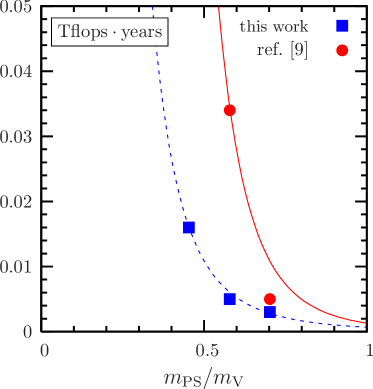
(a) Comparison to ref. [9].

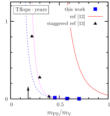
(b) Update of the “Berlin Wall” plots of refs. [12, 13].

Figure 4: Computer resources needed to generate $1000$ independent configurations of size $24^{3}\times 40$ at a lattice spacing of about $0.08\ \mathrm{fm}$ in units of $\mathrm{Tflops}\cdot\mathrm{years}$ as a function of $m_{\mathrm{PS}}/m_{\mathrm{V}}$. In (a) we compare our results represented by squares to the results of ref. [9] represented by circles. The lines are functions proportional to $(m_{\mathrm{PS}}/m_{\mathrm{V}})^{-4}$ (dashed) and $(m_{\mathrm{PS}}/m_{\mathrm{V}})^{-6}$ (solid) with a coefficient such that they cross the data points corresponding to the lightest pseudo scalar mass. In (b) we compare to the formula of eq. 4-7 [12] (solid line) by extrapolating our data with $(m_{\mathrm{PS}}/m_{\mathrm{V}})^{-4}$ (dashed) and with $(m_{\mathrm{PS}}/m_{\mathrm{V}})^{-6}$ (dotted), respectively. The arrow indicates the physical pion to rho meson mass ratio. Additionally, we add points from staggered simulations as were used for the corresponding plot in ref. [13]. Note that all the cost data were scaled to match a lattice time extend of $T=40$.

4.7 Scaling with the mass

An important property of an algorithm for lattice QCD is the scaling of the costs with the simulated quark mass. The naive expectation is that the number of solver iterations grows like $m_{q}^{-1}$ and also the number of molecular dynamics steps is proportional to $m_{q}^{-1}$, see for instance ref. [38] or ref. [12]. Since also the integrated autocorrelation time is assumed to grow like $m_{q}^{-1}$, it is expected that the HMC algorithm costs scale with the quark mass as $m_{q}^{-3}$ or equivalently as $m_{\mathrm{PS}}^{-6}$. In contrast, for our HMC algorithm variant we expect a much weaker scaling of $\Delta\tau$ and also of the number of solver iterations. Indeed, we see that the costs for our HMC algorithm variant is consistent with a $m_{q}^{-2}$ or $m_{\mathrm{PS}}^{-4}$ behaviour when the autocorrelation time is taken into account.

We have translated the number of matrix vector multiplications from table 5 into costs in units $\mathrm{Tflops}\cdot\mathrm{years}$ and plotted the computer resources needed to generate $1000$ independent configurations of size $24^{3}\times 40$ at a lattice spacing of $\sim 0.08\,\mathrm{fm}$ as a function of $m_{\mathrm{PS}}/m_{\mathrm{V}}$ in figure 4(a) together with the results of ref. [9]. Note that we have scaled our costs like $(40/32)^{1.25}$ corresponding to the expected volume dependence (cf. [12]) to match the different time extents and, moreover, we used the plaquette autocorrelation time as an estimate for the autocorrelation time.

The solid (dashed) line is not a fit to the data, but a function proportional to $(m_{\mathrm{PS}}/m_{\mathrm{V}})^{-4}$ ($(m_{\mathrm{PS}}/m_{\mathrm{V}})^{-6}$) with a coefficient that is fixed by the data point corresponding to the lightest pseudo scalar mass. This functional dependencies on $(m_{\mathrm{PS}}/m_{\mathrm{V}})$ describes the data reasonably well. However, from figure 4(a) it is not possible to decide on the value of the exponent in the quark mass dependence of the costs. But, it is clear from the figure that with multiple time scale integration and mass preconditioning the “wall” – which renders simulations at some point infeasible – is moved towards smaller values of the quark mass.

On a larger scale we can compare the extrapolations of our cost data to the formula given in ref. [12]

$$C=K\left(\frac{m_{\mathrm{PS}}}{m_{\mathrm{V}}}\right)^{-z_{\pi}}L^{z_{L}}\ a^{-z_{a}}\,,$$ (4-7)

where the constant $K$ can be found in ref. [12] and $z_{\pi}=6$, $z_{L}=5$ and $z_{a}=7$. The result of this comparison is plotted in figure 4(b), which is an update of the “Berlin Wall” figure that can be found in ref. [13]. We plot the simulation costs in units of $\mathrm{Tflops}\cdot\mathrm{years}$ versus $m_{\mathrm{PS}}/m_{\mathrm{V}}$, where we again scaled the numbers in order to match a lattice time extend of $T=40$. The dashed and the dotted lines are extrapolations from our data proportional to $(m_{\mathrm{PS}}/m_{\mathrm{V}})^{-4}$ and $(m_{\mathrm{PS}}/m_{\mathrm{V}})^{-6}$, respectively, again matching the data point corresponding to the lightest pseudo scalar mass. The solid line corresponds to eq. (4-7). In addition we plot data from staggered simulations as were used for the plot in ref. [13]. That the corresponding points lie nearly on top of the dotted line is accidental.

Conservatively one can conclude from figure 4(b) that with the HMC algorithm described in this paper at least simulations with $m_{\mathrm{PS}}/m_{\mathrm{V}}\approx 0.3$ are feasible, even though $L=1.93\,\mathrm{fm}$ is too small for such values of the masses. Taking the more optimistic point of view by assuming that the costs scale with $z_{\pi}=4$, even simulation with the physical $m_{\mathrm{PS}}/m_{\mathrm{V}}$ ratio and a lattice spacing of $0.08\,\mathrm{fm}$ become accessible, with again the caveat that $L/a$ needs to be increased.

Independent of the value for $z_{\pi}$, figure 4(b) reveals that the costs for simulations with staggered fermions and with Wilson fermions in a comparable physical situation are of the same order of magnitude, if for the simulations with Wilson fermions an algorithm like the one presented in this work is used. It would be interesting to see whether the techniques applied in this paper work similarly well for staggered fermions.

We would like to point out that we did not try to tune the parameters to their optimal values. The aim of this paper was to give a first comparison of mass preconditioned HMC algorithm with multiple time scale integration to existing performance data, i.e. data for a HMC algorithm preconditioned by domain decomposition [8] and data for the HMC algorithm variant of ref. [9]. We are confident that there are still improvements possible by further tuning of the parameters in our variant of the HMC algorithm.

5 Conclusion

In this paper we have presented and tested a variant of the HMC algorithm combining multiple time scale integration with mass preconditioning (Hasenbusch acceleration). The aim of this paper was to perform a first investigation of the performance properties of this HMC algorithm by comparing it to other state of the art HMC algorithm variants at the same situation, i.e. for bare quark masses in the range of $20$ to $60\,\mathrm{MeV}$, a lattice spacing of about $0.08\,\mathrm{fm}$ and a lattice size of $L\approx 2$fm with two flavors of mass degenerate Wilson fermions.

We computed at each simulation point the expectation values of the plaquette and of the pion, the vector and the current quark masses finding full agreement with results in the literature. In order to set the scale we computed the Sommer scale [29], providing a value for $r_{0}/a$ also at the lowest quark mass we simulated and which has not been available in the literature so far.

We have shown that the additional mass parameters introduced for mass preconditioning can be arranged such that the force contributions from the different parts in the Hamiltonian are strictly ordered with respect to the absolute value of the force and that the most expensive part has the smallest contribution to the total force.

Using this result, it is possible to tune the time scales such that the performance of our variant in terms of the cost figure in eq. (4-5) is compatible to the one observed for the HMC algorithm with multiple time scales and domain decomposition as preconditioner introduced in ref. [8] and clearly superior to the one for the HMC algorithm with a simple leap frog integration scheme as used in ref. [9].

While the cost figure provides a clean algorithm performance measure we also compare the simulation costs in units of $\mathrm{Tflops}\cdot\mathrm{years}$ to existing data. This comparison is summarized in an update of the “Berlin wall” plot of ref. [13], which can be found in figure 4. We could show that with the HMC algorithm presented in this paper the wall is moved towards smaller values of the quark mass and that simulations with a ratio of $m_{\mathrm{PS}}/m_{\mathrm{V}}\approx 0.3$ become feasible at a lattice spacing of around $0.08\,\mathrm{fm}$ and $L\approx 2$fm.

The HMC variant presented here has the advantage of being applicable to a wide variety of Dirac operators, including in principle also the overlap operator. In addition its implementation is straightforward, in particular in an already existing HMC code. We remark that the paralllelization properties of our HMC variant and the one of the algorithm presented in [8] can be very different depending on whether a fine- or a coarse-grained massively parallel computer architecture is used.

From a stability point of view our results reveal that even for Wilson fermions it is very well possible to simulate quark masses of the order of $20\ \mathrm{MeV}$ when using the algorithmic ideas presented in this paper. We are presently simulating even smaller quark masses without practical problems, but the statistics is not yet adequate to say something definite.

The results presented in this paper are mostly based on empirical observations and on simulations for only one value of the coupling constant $\beta=5.6$. It remains to be seen how our HMC variant behaves for larger values of $\beta$, which, as well as smaller quark masses and theoretical considerations about the scaling properties with the quark mass needs further investigations.

Moreover, a more systematic study of the interplay between integration schemes, step sizes, (preconditioning and physical) masses and the simulation costs is needed. Those investigations will hopefully also provide a better understanding of the algorithm itself and its dynamics.

Finally, we think that there are further improvements possible by the usage of a Polynomial HMC (PHMC) algorithm [39, 40, 41, 42]. With such an algorithm one could treat the lowest eigenvalues of the Dirac operator exactly and/or by reweighting. In this set-up the large fluctuations in the force might be significantly reduced, if the lowest eigenvalues are responsible for those. Then it might be possible to further reduce the number of inversions of the badly conditioned physical operator needed to evolve the system.

References

- [1] S. Duane, A. D. Kennedy, B. J. Pendleton and D. Roweth, Phys. Lett. B195, 216 (1987).
- [2] T. A. DeGrand and P. Rossi, Comput. Phys. Commun. 60, 211 (1990).
- [3] J. C. Sexton and D. H. Weingarten, Nucl. Phys. B380, 665 (1992).
- [4] R. C. Brower, T. Ivanenko, A. R. Levi and K. N. Orginos, Nucl. Phys. B484, 353 (1997), [hep-lat/9509012].
- [5] M. Hasenbusch, Phys. Lett. B519, 177 (2001), [hep-lat/0107019].
- [6] M. Hasenbusch and K. Jansen, Nucl. Phys. B659, 299 (2003), [hep-lat/0211042].
- [7] M. Lüscher, Nucl. Phys. B418, 637 (1994), [hep-lat/9311007].
- [8] M. Lüscher, Comput. Phys. Commun. 165, 199 (2005), [hep-lat/0409106].
- [9] B. Orth, T. Lippert and K. Schilling, Phys. Rev. D 72 (2005) 014503, [hep-lat/0503016].
- [10] A. Ali Khan et al., Nucl. Phys. Proc. Suppl. 129, 853 (2004), [hep-lat/0309078].
- [11] QCDSF, A. Ali Khan et al., Phys. Lett. B564, 235 (2003), [hep-lat/0303026].
- [12] CP-PACS and JLQCD, A. Ukawa, Nucl. Phys. Proc. Suppl. 106, 195 (2002).
- [13] K. Jansen, Nucl. Phys. Proc. Suppl. 129, 3 (2004), [hep-lat/0311039].
- [14] F. Farchioni et al., Eur. Phys. J. C39, 421 (2005), [hep-lat/0406039].
- [15] M. A. Clark and A. D. Kennedy, hep-lat/0409134.
- [16] ALPHA, M. Della Morte et al., Comput. Phys. Commun. 156, 62 (2003), [hep-lat/0307008].
- [17] TrinLat, M. J. Peardon and J. Sexton, Nucl. Phys. Proc. Suppl. 119, 985 (2003), [hep-lat/0209037].
- [18] TXL, G. S. Bali et al., Phys. Rev. D62, 054503 (2000), [hep-lat/0003012].
- [19] L F , T. Chiarappa et al., in preparation (2005).
- [20] A. Frommer, V. Hannemann, B. Nockel, T. Lippert and K. Schilling, Int. J. Mod. Phys. C5, 1073 (1994), [hep-lat/9404013].
- [21] K. Jansen and C. Liu, Nucl. Phys. Proc. Suppl. 53, 974 (1997), [hep-lat/9607057].
- [22] C. Liu, A. Jaster and K. Jansen, Nucl. Phys. B524, 603 (1998), [hep-lat/9708017].
- [23] R. G. Edwards, I. Horvath and A. D. Kennedy, Nucl. Phys. B484, 375 (1997), [hep-lat/9606004].
- [24] C. Urbach, Untersuchung der Reversibilitätsverletzung im Hybrid Monte Carlo Algorithmus, Diploma thesis, Freie Universität Berlin, Fachbereich Physik, 2002.
- [25] ALPHA, U. Wolff, Comput. Phys. Commun. 156, 143 (2004), [hep-lat/0306017].
- [26] N. Madras and A. D. Sokal, J. Statist. Phys. 50, 109 (1988).
- [27] R. Gupta, G. W. Kilcup and S. R. Sharpe, Phys. Rev. D38, 1278 (1988).
- [28] F. Farchioni, C. Gebert, I. Montvay and L. Scorzato, Eur. Phys. J. C26, 237 (2002), [hep-lat/0206008].
- [29] R. Sommer, Nucl. Phys. B411, 839 (1994), [hep-lat/9310022].
- [30] A. Hasenfratz, R. Hoffmann and F. Knechtli, Nucl. Phys. Proc. Suppl. 106, 418 (2002), [hep-lat/0110168].
- [31] SESAM, G. S. Bali, H. Neff, T. Duessel, T. Lippert and K. Schilling, Phys. Rev. D71, 114513 (2005), [hep-lat/0505012].
- [32] ALPHA, M. Della Morte et al., Phys. Lett. B581, 93 (2004), [hep-lat/0307021].
- [33] M. Della Morte, A. Shindler and R. Sommer, hep-lat/0506008.
- [34] APE, M. Albanese et al., Phys. Lett. B192, 163 (1987).
- [35] S. Fischer et al., Comp. Phys. Commun. 98, 20 (1996), [hep-lat/9602019].
- [36] R. C. Brower, A. R. Levi and K. Orginos, Nucl. Phys. Proc. Suppl. 42, 855 (1995), [hep-lat/9412004].
- [37] M. Lüscher, Comput. Phys. Commun. 156, 209 (2004), [hep-lat/0310048].
- [38] K. Jansen, Nucl. Phys. Proc. Suppl. 53, 127 (1997), [hep-lat/9607051].
- [39] P. de Forcrand and T. Takaishi, Nucl. Phys. Proc. Suppl. 53, 968 (1997), [hep-lat/9608093].
- [40] R. Frezzotti and K. Jansen, Phys. Lett. B402, 328 (1997), [hep-lat/9702016].
- [41] R. Frezzotti and K. Jansen, Nucl. Phys. B555, 395 (1999), [hep-lat/9808011].
- [42] R. Frezzotti and K. Jansen, Nucl. Phys. B555, 432 (1999), [hep-lat/9808038].