HU-EP-05/26
DESY 05-091
SFB/CPP-05-21

Cutoff Effects in O($N$) Nonlinear Sigma Models

Abstract

In the nonlinear O($N$) sigma model at $N=3$ unexpected cutoff effects have been found before with standard discretizations and lattice spacings. Here the situation is analyzed further employing additional data for the step scaling function of the finite volume massgap at $N=3,4,8$ and a large $N$-study of the leading as well as next-to-leading terms in $1/N$. The latter exact results are demonstrated to follow Symanzik’s form of the asymptotic cutoff dependence. At the same time, when fuzzed with artificial statistical errors and then fitted like the Monte Carlo results, a picture similar to $N=3$ emerges. We hence cannot conclude a truly anomalous cutoff dependence but only relatively large cutoff effects, where the logarithmic component is important. Their size shrinks at larger $N$, but the structure remains similar. The large $N$ results are particularly interesting as we here have exact nonperturbative control over an asymptotically free model both in the continuum limit and on the lattice.

1 Introduction

The O($N$) nonlinear sigma models in two space time dimensions are a very precisely studied class of quantum field theories in many respects. For $N\geq 3$ they are asymptotically free like QCD and hence furnish a simplified test laboratory for all kinds of questions. This includes the question of the dependence of physical results on the lattice spacing and this is the subject studied in this publication.

While we are interested in results at zero lattice spacing, nonperturbative Monte Carlo results are always at finite $a$. One hence has to assume an analytical form for the asymptotic $a$-dependence to extrapolate to zero. Ideally this behavior is checked with good precision for a large range of $a$ and then assumed for the ‘remaining’ extrapolation. In principle a systematic error has to be estimated here, which however is often deemed to be negligible compared with statistical errors, which tend to be amplified in the extrapolation. This balance depends on the ‘extrapolation fit’ one uses. If it is restrictive with few parameters (but compatible with the data) statistical errors remain small but the danger of systematic effects is high. In the opposite case one may ‘give away’ statistical precision and overestimate total errors. It is presumably clear from these words that in the extrapolation step there is some danger of subjective elements getting into a presumed ‘first principles’ calculation. The situation is aggravated in QCD with dynamical fermions, because due to algorithmic and CPU-power limitations one cannot vary $a$ over a large enough range. Continuum results then mainly arise under the assumption of a certain $a$-dependence.

Almost universally in lattice field theory the model of the asymptotic cutoff dependence is derived from Symanzik’s analysis of lattice perturbation theory to all orders [1]. It extends the investigation of renormalizability to subleading orders in the cutoff and is assumed to hold in structure also beyond perturbation theory and to thus ascertain the existence of the continuum limit and predict the rate at which it is approached. The results for the rate are powers in $a$ (usually $a^{2}$ or linear for fermions) modulated by only slowly varying logarithmic factors.

In view of this situation there have been efforts to explore this in detail in the sigma model lab. The situation there is vastly better than in QCD: No critical slowing down due to cluster algorithms [2] , well-understood and well-measurable finite size quantities [3], reduced variance estimators [4]. The Symanzik prediction for this bosonic theory is clearly $a^{2}$ scaling. In earlier investigations [5, 6] it has been found that some results of the O(3) model do not fit very well with this standard expectation down to rather small $a$-values. These studies are extended here in the direction of larger $N$-values, since it is known analytically that eventually at $N=\infty$ the Symanzik picture holds. We here report in Sect. 2 Monte Carlo results for $N=3,4,8$ with the standard lattice discretization. In Sect. 3 we investigate the large $N$ expansion including the leading correction of order $1/N$. In Sect. 4 we draw some conclusions.

2 Monte Carlo Data

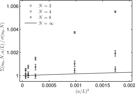
Figure 1: Lattice step scaling function $\Sigma(u_{0},N,a/L)$ normalized by the continuum value $\sigma(u_{0},N)$ at $u_{0}=1.0595$.

We consider the lattice O($N$) nonlinear $\sigma$-model

$$Z=\int\prod_{x}d^{N}s\delta(s^{2}-1)\mathrm{e}^{-S(s)}$$ (1)

with the standard lattice action

$$S(s)=\frac{N}{2\gamma}\sum_{x\mu}(\partial_{\mu}s)^{2}$$ (2)

where $\partial_{\mu}$ is the forward difference operator and $\gamma$ the rescaled coupling (fixed at large $N$). Both in our MC simulations and the large $N$ expansion we determine the step scaling function (for a factor two rescaling)

$$\Sigma(u,N,a/L)=M(2L)\,2L\,,\qquad u=M(L)\,L\,,$$ (3)

where $M(L)$ is the mass-gap [7] of the transfer matrix. It is determined from the asymptotic exponential fall-off of the two-point function at zero spatial momentum. In principle this refers to a periodic box with finite spatial size $L$ and infinite extent in the time direction. In the simulations this was approximated as described in [3]. The renormalized coupling $M(L)L$ used here differs by a factor $(N-1)/2$ from $\bar{g}^{2}(L)$ in [3] to keep it finite in the large $N$ limit. The lattice step scaling function is expected to reach a finite continuum limit,

$$\lim_{a/L\to 0}\Sigma(u,N,a/L)=\sigma(u,N)$$ (4)

and we discuss here how this is approached. At large $N$ we shall use the expansion

$$\Sigma(u,N,a/L)=\Sigma_{0}(u,a/L)+\frac{1}{N}\,\Sigma_{1}(u,a/L)+\mathrm{O}(N^{-2}).$$ (5)

$L/a$	$\Sigma(u_{0},3,a/L)$	$\Sigma(u_{0},4,a/L)$	$\Sigma(u_{0},8,a/L)$	$\Sigma_{0}(u_{0},a/L)$	$\Sigma_{1}(u_{0},a/L)$
5	1.29379(8)		-	-	-
6	-	1.31256(47)	1.35065(40)	1.379491	-0.194123
8	-	1.31068(43)	1.34891(35)	1.378215	-0.196201
10	1.27994(9)	1.30825(39)	1.34835(34)	1.377524	-0.197668
12	1.27668(9)	1.30608(37)	1.34721(32)	1.377112	-0.198665
16	1.27228(12)	1.30477(34)	1.34725(30)	1.376665	-0.199867
24	1.26817(9)	1.30379(32)	1.34649(28)	1.376309	-0.200939
32	1.26591(9)	1.30263(31)	1.34635(27)	1.376170	-0.201394
64	1.26306(16)	1.30225(32)	1.34570(25)	1.376022	-0.201921
96	1.26216(18)	1.30138(33)	1.34577(24)	1.375990	-0.202042
128	1.26187(13)	1.30149(34)	1.34563(24)	1.375978	-0.202089
cont.	1.261208(1)	1.3012876(1)	1.345757(2)	1.375961	-0.202161

Table 1: Monte Carlo and large $N$ data for the lattice step scaling function at $u_{0}=1.0595$.

For technical details about our algorithm and estimators used in the simulations we refer the reader to Ref. [8]. Results are listed in Table 1. The O(3) data for $L/a\leq 64$ has been taken from [6], where Seefeld et. al. study cutoff effects in $\Sigma(u_{0},3,a/L)$ at the popular value $u_{0}=1.0595$ already appearing in [3]. We have extended their data to the lattices $L/a=96,\,128$ and have added results at $N=4,8$ to explore the transition to the large $N$ behaviour that we later study semi-analytically. The bottom line of the table contains proposed exact continuum values published in [9] for $N=3$ and the values for $N=4,8$ [10]. They depend on some mild theoretical assumptions, but look consistent with our numerical values [8, 9]. More precisely, an extrapolation with the fit-forms considered below (eqns. (6) – (8)) leads to extrapolated values that agree with the conjectured exact values within errors (propagated from the Monte Carlo statistical errors) as soon as the $\chi^{2}$ of the fit is acceptable. More details can be found in [8]. In this publication we assume the conjectured continuum values to be correct and use them to constrain our extrapolations. We notice that the case $N=8$ is very well described by the large $N$ expansion. Values of $\Sigma$ at $N=8$ and $N=\infty$ differ by about 2.2%. This discrepancy is lowered to about $0.4\%$ by the $1/N$ correction that we shall derive in this paper.

We have a first look at cutoff effects in Fig. 1 where we simply plot $\Sigma/\sigma$ versus $(a/L)^{2}$ for the different values of $N$ together with the exact curve for $N=\infty$. Again $N=8$ is already close to the large $N$ limit. The lattice artifacts for $N>3$ generally turn out to be much smaller than for $N=3$, which makes the numerical investigation of their structure more difficult. While the $N=3$ data look curved to the naked eye in this representation, this cannot be decided so easily for the higher $N$-values. In order to analyze the cutoff effects in more detail we will fit several analytic forms to the data. In the following Section we explain what kind of fits we have done and how and what we can learn from them.

2.1 Fits to the data

Symanzik’s analysis of the cutoff dependence of lattice Feynman diagrams suggests that leading lattice artifacts are quadratic in the lattice spacing modified by slowly varying logarithmic functions. It should be noted however that logarithms generically appear in an $l$’th order polynomial at $l$ loop order. If the series were summable the leading power could thus be modified. Nevertheless in typical lattice applications it is assumed that the integer power behaviour is modified only weakly and that this can be neglected for most attainable statistical precisions in an extrapolation. It was first found in [5] that in the O(3) model instead of the expected quadratic dependence a behaviour more close to a linear is suggested. With this background we first investigate fits with a general exponent $\alpha$

$$\mathrm{A}:\quad c_{0}+c_{1}\,(a/L)^{\alpha}\,,$$ (6)

where $c_{0}$ is fixed by our exact continuum data. Such a fit results in an optimal exponent $\alpha_{\mathrm{opt}}$ that minimizes the $\chi^{2}$ deviation between (6) and the data. To judge the plausibility of such a fit we compute the probability $Q$ of finding a value of $\chi^{2}$ larger or equal to the one encountered in the fit at hand (goodness of fit test [11]). In general, values $Q<0.1$ are considered implausible.

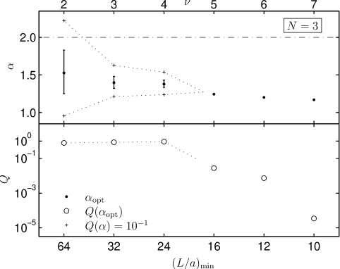
Figure 2: Results of the fit to eq. (6) for $N=3$. In the upper half the optimal exponent and the limits where the fit with fixed $\alpha$ becomes unlikely is plotted. The lower half shows $Q(\alpha_{\mathrm{opt}})$. The dotted lines are to guide the eye.

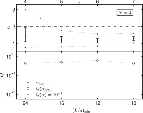
Figure 3: As Fig. 2 but for $N=4$.

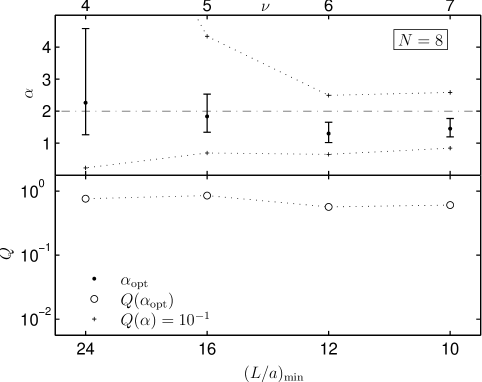
Figure 4: As Fig. 2 but for $N=8$.

For $N=3$ fit results are shown in Fig. 2 which requires some explanation. Since all theoretical forms of the cutoff behavior are only asymptotic, we successively exclude coarser lattices from the fit. We therefore find values $\alpha$ and $Q$ as functions of $(L/a)_{\mathrm{\min}}$, the size in lattice units of the coarsest lattice still included in the fit. The top labels list the numbers $\nu$ of the remaining degrees of freedom in the fit. Errors of $\alpha_{\mathrm{opt}}$ are assessed in two ways. The errorbars are limited by those values of $\alpha$ where the optimal $\chi^{2}$ grows by unity. The plus signs are the limits where $Q$ falls below 0.1. When there are no fits with $Q\geq 0.1$ no errors are drawn. We see here that acceptable fits are only achieved with lattices $L/a\geq 24$. Moreover they are neither consistent with the Symanzik value $\alpha=2$ (dash-dotted line) nor with $\alpha=1$ but rather favor values in between. For $N=4,8$ the equivalent plots are shown in Fig. 3 and Fig. 4. In these cases the proposed fit is acceptable for all $(L/a)_{\mathrm{\min}}\geq 10$. For $N=4$ the preferred $\alpha$-values are still smaller than two, but $N=8$ starts to look consistent with the whole range between one and two.

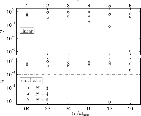
Figure 5: $Q$-values of the fits to eq. (7) (linear) and eq. (8) (quadratic) against $(L/a)_{\mathrm{\min}}$. For $N=4\,,8$ both fits are perfect in the whole range. For $N=3$ both fits start to become unlikely at $(L/a)_{\mathrm{\min}}=12$.

In addition to fit A with a general correction to scaling exponent we also tried the Symanzik and the ad hoc linear form with both including the simplest logarithmic correction

$$\mathrm{B}: c_{0}+c_{1}\,(a/L)\phantom{{}^{2}}+c_{2}\,(a/L)\phantom{{}^{2}}\,\ln(a/L)\,.$$ (7)

$$\mathrm{C}: c_{0}+c_{1}\,(a/L)^{2}+c_{2}\,(a/L)^{2}\,\ln(a/L)\,,$$ (8)

Note that at $N=\infty$ the form C is known to apply (see next section). In the upper and the lower subplot of Fig. 5 the $Q$-values are shown for the linear (eq. (7)) and quadratic (eq. (8)) form respectively. For $N=4,\,8$ both fits are tolerable in the whole $(L/a)_{\mathrm{\min}}$-range. In the case $N=3$ and at small $(L/a)_{\mathrm{\min}}$ both forms become unlikely. For $(L/a)_{\mathrm{\min}}=16$ the form C, with quadratic lattice artifacts, gives the better fit, but for $(L/a)_{\mathrm{\min}}=12$ it is already intolerable whereas the linear fit with $Q\approx 10^{-1}$ could perhaps still be accepted.

In summary, the single exponent ansatz A hints at ‘effective’ values between one and two in the range of cutoffs studied. With logarithmic modifications inluded, linear and quadratic dependence is asymptotically about equally well compatible with our data. All fits studied here have at most two free parameters. More complicated fits can be extended to coarser lattices, and then the additional parameters are actually largely determined by these additional included data. We do not think that much can be learnt from such more involved fits. We rather turn now to the study of large $N$ to then apply the same fitting procedure in a case where we have additional insight in the true cutoff dependence.

3 O($N$) model at large $N$

At finite $N$ Monte Carlo simulations were our tool to go beyond perturbation theory. In this section we complement this information by evaluating the first two terms of the $1/N$ expansion of the step scaling function. As we shall discuss they are nonperturbative in the renormalized coupling $M(L)L$. Related large $N$ computations are found for example in [12] and [13], but to our knowledge the step scaling function as defined here and in particular its subleading correction is not in the literature.

For simplicity we employ lattice units in the following with the lattice spacing set to $a=1$. Scaling is then studied in $1/L$.

3.1 Spin correlation function

To extract the mass-gap we need to study the spin two-point function. We Fourier represent the spin constraints in (1) and add a source term to obtain the generating functional of spin correlation functions

$$Z(J)=\int\prod_{x}d^{N}s\frac{d\alpha}{2\pi i}\mathrm{e}^{-S(s)-(\alpha,s^{2}-1)+(J,s)}$$ (9)

with each $\alpha(x)$ integrated along the imaginary axis. We rescale $\alpha$, shift contours $\alpha(x)=m_{0}^{2}+i\varphi(x)$ and perform the Gaussian $s$-integrals to obtain

$$Z(J)\propto\int\prod_{x}d\varphi\mathrm{e}^{-S_{\operatorname{eff}}(\varphi)+\frac{\gamma}{2N}(J,K^{-1}J)}$$ (10)

with

$$S_{\operatorname{eff}}(\varphi)=\frac{N}{2}\operatorname{tr}\log K-\frac{iN}{2\gamma}\sum_{x}\varphi$$ (11)

involving the operator

$$K=-\partial_{\mu}\partial_{\mu}^{\ast}+m_{0}^{2}+i\varphi\equiv(D^{-1}+i\varphi)=D^{-1}(1+iD\varphi),$$ (12)

where the scalar field $\varphi$ is regarded as a diagonal matrix and

$$D=(-\partial_{\mu}\partial_{\mu}^{\ast}+m_{0}^{2})^{-1}.$$ (13)

The mass $m_{0}^{2}$ is chosen such that $\alpha(x)=m_{0}^{2}$ is a saddlepoint or equivalently, that $S_{\operatorname{eff}}(\varphi)$ is minimal for $\varphi=0$. This occurs if the gap equation

$$\frac{1}{\gamma}=\frac{1}{V}\operatorname{tr}K^{-1}|_{\varphi=0}=\frac{1}{V}\operatorname{tr}D$$ (14)

is fulfilled with the volume $V$ equaling the number of lattice sites.

Next we expand $S_{\operatorname{eff}}$ in powers of $\varphi$, omit a constant and rescale $\varphi\rightarrow\sqrt{2/N}\varphi$ to find

$$S_{\operatorname{eff}}(\varphi)=\left[\frac{1}{2}\operatorname{tr}(D\varphi)^{2}-\frac{i}{3}\sqrt{\frac{2}{N}}\operatorname{tr}(D\varphi)^{3}-\frac{1}{2N}\operatorname{tr}(D\varphi)^{4}+\ldots.\right].$$ (15)

Similarly we then get

$$K^{-1}=D-i\sqrt{\frac{2}{N}}D\varphi D-\frac{2}{N}D\varphi D\varphi D+\ldots.$$

The spin two point function is given by

$$\left\langle s_{i}(x)s_{j}(y)\right\rangle=\frac{\gamma}{N}\delta_{ij}G(x,y),$$

$$G(x,y)=\left\langle K^{-1}(x,y)\right\rangle$$

with the expectation value taken with $S_{\operatorname{eff}}$ and employing an obvious kernel notation for the operator $K^{-1}$. Upon $1/N$ expansion this implies

$$G=D-\frac{2}{N}\left\langle D\varphi D\varphi D\right\rangle_{0}+\frac{2}{3N}\left\langle D\varphi D\operatorname{tr}(D\varphi)^{3}\right\rangle_{0}+O(N^{-2})$$ (16)

with $\left\langle\ldots\right\rangle_{0}$ taken now with only the quadratic part of $S_{\operatorname{eff}}$. We introduce the selfenergy operator $H=\frac{1}{N}H_{1}+O(1/N^{2})$ by setting

$$G^{-1}=D^{-1}+H$$ (17)

and read off by comparing with (16)

$$H_{1}=2\left\langle\varphi D\varphi\right\rangle_{0}-\frac{2}{3}\left\langle\varphi\operatorname{tr}(D\varphi)^{3}\right\rangle_{0}\equiv H_{1,a}+H_{1,b}.$$ (18)

Going to momentum space with

$$\tilde{D}(p)=\frac{1}{\hat{p}^{2}+m_{0}^{2}},\quad\text{$\hat{p}_{\mu}=2\sin(p_{\mu}/2)$}$$ (19)

and the $\varphi$-propagator $\tilde{W}(p)$ determined in the first term in (15) as

$$\tilde{W}^{-1}(p)=\frac{1}{V}\sum_{q}\tilde{D}(p-q)\tilde{D}(q),$$ (20)

the two contributions have the form

$$\tilde{H}_{1,a}(p)=\frac{2}{V}\sum_{q}\tilde{D}(q)\tilde{W}(q-p)$$ (21)

and

$$\tilde{H}_{1,b}=-\tilde{W}(0)\frac{2}{V^{2}}\sum_{q,r}\tilde{W}(q)\tilde{D}(q-r)\tilde{D}^{2}(r).$$ (22)

Figure 6: Diagrammatic representation of (21) and (22).

These terms are visualized by the diagrams in Fig. 6 where $\tilde{D}$ is represented by solid and $W$ by wiggly lines. Using the explicit form of $\tilde{D}$ we can eliminate the double sum in the constant $\tilde{H}_{1,b}$ and find

$$\tilde{H}_{1,b}=\tilde{W}(0)\frac{1}{V}\sum_{q}\tilde{W}(q)\frac{\partial}{\partial m_{0}^{2}}\tilde{W}^{-1}(q).$$ (23)

3.2 Mass gap

For our two-dimensional volume $V=TL$ we now take the limit $T\rightarrow\infty$. The momentum $p_{0}$ becomes continuous and we have to replace

$$\frac{1}{V}\sum_{p}\ldots.\rightarrow\frac{1}{L}\sum_{p_{1}}\int\frac{dp_{0}}{2\pi}\ldots.$$

The gap equation becomes in this limit

$$\frac{1}{L}\sum_{p_{1}}\int\frac{dp_{0}}{2\pi}\frac{1}{\hat{p}^{2}+m_{0}^{2}}=\frac{1}{L}\sum_{p_{1}}\frac{1}{2\hat{\omega}(p_{1})\sqrt{1+\hat{\omega}^{2}(p_{1})/4}}=\frac{1}{\gamma}$$ (24)

with $\hat{\omega}^{2}(p_{1})=(\hat{p}_{1}^{2}+m_{0}^{2})$. It furnishes a one-to-one relation (at given $L$) between $m_{0}^{2}$ and $\gamma>0$.

The mass gap $M>0$ of the transfer matrix can be extracted from the two point function in momentum space $\tilde{G}(p)$ by finding the smallest real $M$ with

$$\tilde{G}^{-1}(p_{M})=0,\quad p_{M}=(iM,0).$$ (25)

We expand

$$M=M_{0}+\frac{1}{N}M_{1}+\ldots.$$ (26)

At leading order $G$ coincides with $D$ which yields

$$M_{0}=\ln\left[1+m_{0}\sqrt{1+m_{0}^{2}/4}+m_{0}^{2}/2\right]=M_{0}(\gamma,L).$$ (27)

If we now combine (25), (26), (17) we obtain for the first correction to the mass

$$M_{1}=\frac{\tilde{H}_{1}(p_{M_{0}})}{2m_{0}\sqrt{1+m_{0}^{2}/4}}.$$ (28)

In the practical evaluation $M_{0}(\gamma,L)$ follows easily from solving (24) for instance by the Newton Raphson algorithm. For the correction it is essential that also the $T\rightarrow\infty$ limit of $\tilde{W}$ can be taken in closed form. In a first step we write it as a contour integral in $z=\mathrm{e}^{iq_{0}}$ over the unit circle

$$\tilde{W}^{-1}(p)=\frac{1}{L}\sum_{q_{1}}\oint\frac{dz}{2\pi iz}\frac{1}{2\cosh(\theta)-z-z^{-1}}\frac{1}{2\cosh(\delta)-zz_{0}-z^{-1}z_{0}^{-1}}.$$

Here we have introduced

$$z_{0}=\mathrm{e}^{-ip_{0}},\quad\cosh(\delta)=1+\hat{\omega}^{2}(q_{1}-p_{1})/2,\quad\cosh(\theta)=1+\hat{\omega}^{2}(q_{1})/2.$$

After some algebraic simplifications we arrive at

$$\tilde{W}^{-1}(p)=\frac{1}{2L}\sum_{q_{1}}\frac{\coth(\theta)+\coth(\delta)}{4\sinh^{2}\left(\frac{\theta+\delta}{2}\right)+\hat{p_{0}}^{2}}.$$ (29)

With this form the computation of both $\tilde{H}_{1,a}(p_{M_{0}})$ and $\tilde{H}_{1,b}$ in (21) and (23) leaves us with a single numerical integration over $q_{0}\in[0,\pi]$ (using symmetry) in combination with a two-fold summation over the spatial momenta. This is easily feasible on a PC with high precision and up to $L$ of a few hundred. Between the two diagrams a divergence $\propto L^{2}$ cancels.

A final remark concerns the continuation of $\tilde{H}_{1,a}$ to imaginary momentum. For real momenta $p$ we can obviously use the shifted form

$$\tilde{H}_{1,a}(p)=\frac{2}{L}\sum_{q_{1}}\int\frac{dq_{0}}{2\pi}\tilde{D}(q+r)\tilde{W}(q-p+r)$$

instead of (21) with any admissable lattice momentum $r$ (real $r_{0}$, $r_{1}=2\pi n/L$) including the case $r=p$. Only in the latter case we encounter a singularity if then we simply substitute $p\to p_{M_{0}}$ and a more careful continuation would be required. We used (21) in its original form amounting to $r=0$.

3.3 Step scaling function

We can now determine the coefficients of the expansion (5). For the leading term we read off [14]

$$\Sigma_{0}(u,L)=2LM_{0}(\gamma,2L)|_{LM_{0}(\gamma,L)=u}$$ (30)

with $\gamma$ determined by $u$. For the next term we find (with the same $\gamma$)

$$\Sigma_{1}(u,L)=2LM_{1}(\gamma,2L)-LM_{1}(\gamma,L)\frac{\partial\Sigma_{0}(u,L)}{\partial u},$$ (31)

where the derivative is evaluated in the form

$$\frac{\partial\Sigma_{0}(u,L)}{\partial u}=\frac{2\frac{\partial M_{0}(\gamma,2L)}{\partial\gamma}}{\frac{\partial M_{0}(\gamma,L)}{\partial\gamma}}.$$ (32)

The derivatives $\partial M_{0}/\partial\gamma$ follow from (27) and $\gamma$-derivatives on both sides of (24) avoiding the need to take any derivative numerically.

Each term in the expansion is expected to have a continuum limit for fixed $u$

$$\sigma_{i}(u)=\lim_{L\rightarrow\infty}\Sigma_{i}(u,L)$$ (33)

3.4 Infinite $N$

3.4.1 Continuum

At leading order the step scaling function is given just by the gap equation. In ref.[12] we find asymptotic large $L$ expansions of lattice sums relevant for (24) that yield

$$\frac{2}{\gamma}=\frac{1}{\pi}\left[\ln L+G_{0}(u/2\pi)\right]+\frac{1}{u}+C-\frac{u^{2}}{8\pi^{2}}\frac{\ln L}{L^{2}}+\mathrm{O}(1/L^{2}).$$ (34)

Here $C$ is some constant and $G_{0}$ is given by

$$G_{0}(\alpha)=\sum_{n=1}^{\infty}\left[\frac{1}{\sqrt{n^{2}+\alpha^{2}}}-\frac{1}{n}\right].$$ (35)

Note that the Symanzik form of the leading lattice artifacts holds here for all couplings. The exact continuum step scaling function $\sigma_{0}(u)$ is given by the transcendental equation

$$\frac{1}{\pi}\left[\ln 2+G_{0}(\sigma_{0}/2\pi)\right]+\frac{1}{\sigma_{0}}=\frac{1}{\pi}G_{0}(u/2\pi)+\frac{1}{u}.$$ (36)

The function $G_{0}$ possesses a perturbative expansion, convergent for $\alpha<1$,

$$G_{0}(\alpha)=\sum_{n=1}^{\infty}\frac{(2n)!}{(n!)^{2}}\zeta(2n+1)(-\alpha^{2}/4)^{n}$$ (37)

which implies the expansion coefficients of $\sigma$ to all orders. The first ones in

$$\sigma_{0}=u+s_{0}u^{2}+s_{1}u^{3}+\ldots$$ (38)

are

$$s_{0}=\frac{\ln 2}{\pi},\quad s_{1}=s_{0}^{2},\quad s_{2}=s_{0}^{3},\quad s_{3}=s_{0}^{4}-s_{0}\frac{\zeta(3)}{4\pi^{3}},\quad s_{4}=s_{0}^{5}-s_{0}^{2}\frac{7\zeta(3)}{8\pi^{3}}.$$ (39)

In ref.[15] the four loop $\beta$-function at finite $N$ was computed for the LWW coupling. Its $N\rightarrow\infty$ limit yields an expansion for the step scaling function that coincides with the present series and from $s_{3}$ we find for a constant that was determined numerically before the compatible result $\chi_{1}=-\zeta(3)=-1.20\ldots$. Note that for the quantities considered here we confirm the interchangeability of the large $N$- and the cutoff-limit leading to renormalized perturbation theory.

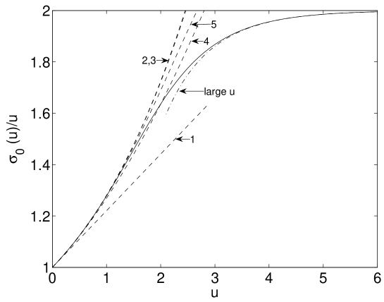
Figure 7: Exact infinite $N$ step scaling function $\sigma_{0}$ together with perturbative and large $u$ approximations. Labels $1,2,\ldots$ denote the expansion (38) including terms up to $s_{0},s_{1},\ldots$ and agree with the loop-order in conventional perturbation theory.

At large $\alpha$ the function (35) has an asymptotic expansion [12]

$$G_{0}(\alpha)=-\ln(\alpha/2)-\frac{1}{2\alpha}+2\sum_{n=1}^{\infty}K_{0}(2\pi n\alpha)+\gamma_{\rm E}$$ (40)

with Euler’s constant $\gamma_{\rm E}$ and the modified Bessel function $K_{0}$. It implies the usual exponential corrections to the finite volume mass gap

$$\sigma_{0}(u)\cong 2u\left[1-2K_{0}(u)\right]\cong 2u\left[1-\sqrt{2\pi/u}\exp(-u)\right].$$ (41)

In Fig. 7 we plot the exact continuum step scaling function together with its small and large $u$ expansions. We remark that a few orders of perturbation theory approximate $\sigma_{0}$ well up to $u\lessapprox 1.5$.

Eq. (36) can of course also be analyzed for other rescaling factors then two. In particular from infinitesimal rescaling we obtain the nonperturbative $\beta$-function in the form

$$\beta(u)=-\frac{u^{2}}{\pi}\frac{1}{1-\frac{u^{2}}{2\pi^{2}}G_{0}^{\prime}(u/2\pi)}+\mathrm{O}(1/N).$$ (42)

3.4.2 Lattice artifacts

At finite $L$ we compute $\Sigma_{0}(u,L)$ exactly by using (24) twice (with $L$ and $2L$), eliminating $\gamma$ and expressing $m_{0}$ by $M_{0}$ via the inverse of (27), $m_{0}=2\,\sinh(M_{0}/2)$. This is implemented numerically to machine precision. Another possibility is the small volume expansion of the gap equation (24) yielding

$$\frac{2}{\gamma}=\frac{1}{u}\left(1+\sum_{n\geqslant 1}d_{n}(L)u^{n}\right)=\frac{1}{\Sigma_{0}}\left(1+\sum_{n\geqslant 1}d_{n}(2L)\Sigma_{0}^{n}\right)$$ (43)

with

$$d_{1}=\frac{1}{L}\sum_{p_{1}\neq 0}\frac{1}{\hat{p}_{1}\sqrt{1+\hat{p}_{1}^{2}/4}},\quad d_{3}=-\frac{1}{2L^{3}}\sum_{p_{1}\neq 0}\frac{1+\hat{p}_{1}^{2}/2}{\hat{p}_{1}^{3}(1+\hat{p}_{1}^{2}/4)^{3/2}},$$ (44)

$$d_{2}=-\frac{1}{6L^{2}},\quad d_{4}=\frac{7}{360L^{4}}.$$ (45)

Numerically we find by the method of App. D of ref.[16]

$$d_{1}(L)=\frac{\ln L}{\pi}-0.0703275870013+0.0872665\frac{1}{L^{2}}+\mathrm{O}(L^{-4})$$ (46)

and

$$d_{3}(L)=-0.0048460224504-\frac{1}{8\pi}\frac{\ln L}{L^{2}}+0.0220539\frac{1}{L^{2}}+\mathrm{O}(L^{-4})$$ (47)

with errors expected to lie beyond the quoted digits.

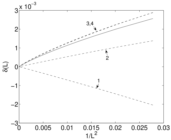
Figure 8: Deviation of $\Sigma_{0}$ from the continuum limit at $u_{0}=1.0595$.

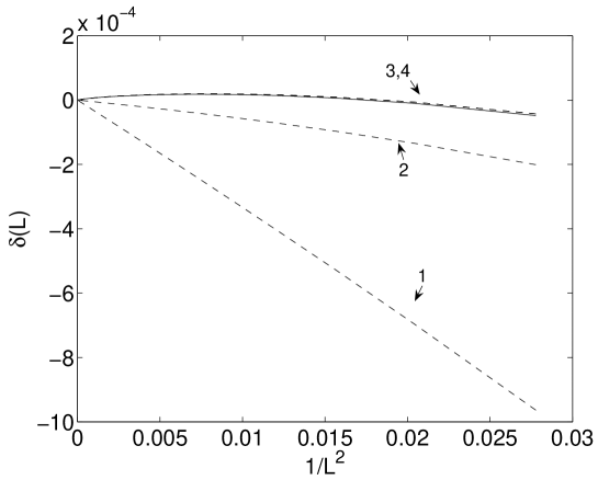
Figure 9: As Fig. 8, but for $u=0.5$.

In view of applications of the step scaling technique for QCD it is interesting to compare the exact lattice artifacts with their perturbative expansion. We form the relative deviation

$$\delta(u,L)=\frac{\Sigma_{0}-\sigma_{0}}{\sigma_{0}}=\delta_{1}(L)u+\delta_{2}(L)u^{2}+\ldots.$$ (48)

Setting

$$\Delta d_{i}(L)=d_{i}(2L)-d_{i}(L)$$ (49)

and combining series we find

$$\delta_{1}(L)=\Delta d_{1}(L)-s_{0},$$ (50)

$$\delta_{2}(L)=\Delta d_{2}(L)-s_{1}+s_{0}^{2}+\Delta d_{1}(L)\delta_{1}(L),$$ (51)

and similar but lengthy expressions for $\delta_{3,4}(L).$ In Fig. 8 the exact $\delta(L)$ is plotted together with perturbative approximations at $u_{0}=1.0595$. While the continuum limit in this range is well described by perturbation theory, this is not really the case for $\delta$. The same was observed in [3] at $N=3$. The leading term does not even have the right sign. This situation improves at yet smaller couplings as shown in Fig. 9. Heuristically, with $\delta$ being a short distance quantity, we thought it might be a good idea to reexpand it in the bare coupling $\gamma(u,L)$ which is always known nonperturbatively in computations of step scaling functions. This experiment did however not lead to a more accurate perturbative description of $\delta$ in the present case.

3.5 $1/N$ correction

For a number of $u$-values we numerically determined $\Sigma_{1}(u,L)$ up to $L=128$ and higher for $u_{0}$. Larger values are possible with some effort, but are of limited use unless also the precision is raised beyond 64 bits. Sofar we have not succeeded in analytically extracting the large $L$-behavior and therefore perform a numerical analysis here.

The expected form is

$$\Sigma_{1}(u,L)=\sigma_{1}(u)+\frac{1}{L^{2}}\Sigma_{1}^{(2)}(u,L)+\frac{1}{L^{4}}\Sigma_{1}^{(4)}(u,L)+\mathrm{O}(L^{-6})$$ (52)

where the $\Sigma_{1}^{(k)}$ have an only weak residual $L$-dependence. For the entirely analogous expansion of the leading $\Sigma_{0}$ it rigorously follows from [12] that $\Sigma_{0}^{(2)}$ is a linear and $\Sigma_{0}^{(4)}$ a quadratic polynomial in $\ln(L)$.

In terms of the symmetric difference

$$\tilde{\Delta}f(L)=\frac{1}{2}(f(L+1)-f(L-1))$$ (53)

we define similarly to [17] ‘blocked functions’

$$B_{i}^{(2)} = -\frac{1}{2}L^{3}\tilde{\Delta}\Sigma_{i}$$ (54)

$$B_{i}^{(4)} = -\frac{1}{16}L^{4}(2+L\tilde{\Delta})^{2}L\tilde{\Delta}\Sigma_{i}$$ (55)

for $i=0,1$. The reasoning behind this construction is that in $B_{0}^{(2)}$ the continuum part of $\Sigma_{0}$ has been canceled and the $L^{-2}$ components are promoted to order unity. The normalization is such that the coefficient of the term linear in $\ln L$ in $\Sigma_{0}^{(2)}$ is the same as in $B_{0}^{(2)}$. Similarly in $B_{0}^{(4)}$ the $L^{-2}$ components are canceled and the coefficient of $(\ln L)^{2}/L^{4}$ is preserved. Although the a priori form of $\Sigma_{1}^{(k)}$ is not analytically known sofar, we construct $B_{1}^{(k)}$ in the same way.

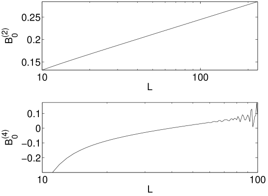
Figure 10: Variation of $L^{-2}$ and $L^{-4}$ components in $\Sigma_{0}(u_{0},L)$.

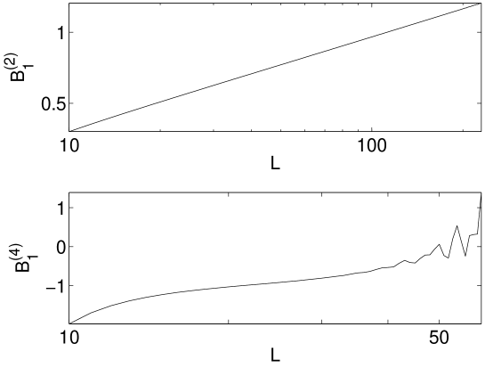
Figure 11: As Fig. 10 but for the subleading term $\Sigma_{1}$

In Fig. 10 we plot $B_{0}^{(k)}$ at $u=u_{0}$ for a range of $L$ and see the expected slowly varying $L$ dependence. The analogous plot Fig. 11 for the $1/N$ correction shows a rather similar structure. Both lower plots eventually start to become irregular at large $L$ due to roundoff noise. For both terms $\Sigma_{i}^{(2)}$ looks strictly linear in $\ln L$ and the $(\ln L)^{2}$ components in $\Sigma_{i}^{(4)}$, i. e. the curvature at large $L$, seems to be very weak. For other $u$-values the situation is qualitatively similar, although coefficients are larger for larger $u$.

After this more qualitative investigation we obtain the coefficients in the asymptotic expansion

$$\Sigma_{1}(u,L)=\sigma_{1}(u)+A(u)\frac{\ln{L}}{L^{2}}+B(u)\frac{1}{L^{2}}+\mathrm{O}(L^{-4})$$ (56)

by the method introduced in [16]. The resulting numbers are collected in Tab.2 and the continuum values are plotted in Fig. 12. The correction obviously has to (and does) vanish for $u\to 0,\infty$ since $\sigma(u,N)$ assumes $N$-independent trivial limits $u$ and $2u$.

It seems rather difficult but perhaps not hopeless to analytically derive the asymptotic $L$-dependence of $\Sigma_{1}$. We hope to come back to such an analysis in a future publication [18].

$u$	$\sigma_{1}$	$A$	$B$
0.5	-0.055886	0.012	-0.066
1	-0.187974	0.220	-0.184
1.0595	-0.202161	0.284	-0.200
1.5	-0.227820	1.27	-0.442
1.75	-0.158761	2.23	-0.84
2	-0.046463	3.26	-1.56
2.25	0.072185	4.13	-2.52
2.5	0.167824	4.67	-3.53(1)
3	0.258377	4.82	-5.12(1)
3.5	0.251671(1)	4.21(1)	-5.71(3)
4	0.205320	3.38(1)	-5.50(4)
4.5	0.152853	2.58(1)	-4.85(4)
5	0.107791	1.92(1)	-4.04(4)
5.5	0.073422	1.40(1)	-3.24(4)
6	0.048858	1.01(1)	-2.52(4)

Table 2: Continuum extrapolation of $\Sigma_{1}$, see eq.(56)

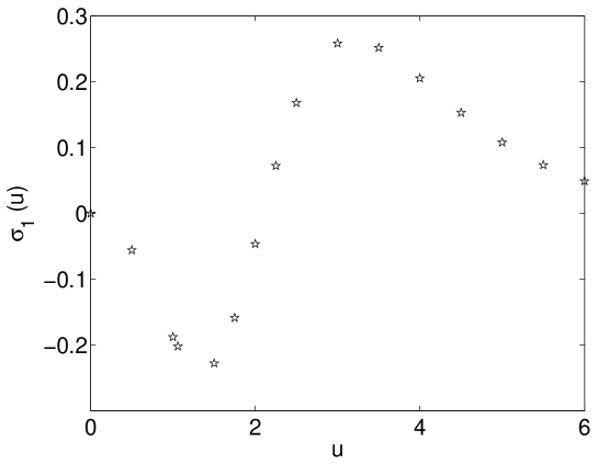
Figure 12: Leading correction $\sigma_{1}(u)$.

It is instructive to perform with our large $N$ data the same analysis as for the Monte Carlo data. For this purpose we ‘fuzz’ our data with artificial errors. For instance we add to $\Sigma_{1}(u_{0},L)$ in the range $10\leq L\leq 128$ Gaussian random numbers of width $2\times 10^{-5}$. This size is chosen such that the lattice artefact $|\Sigma_{1}(u_{0},10)-\sigma_{1}(u_{0})|$ of the $1/N$ correction gets a relative ‘statistical’ error similar to the $N=3$ case. The resulting plot analogous to Fig. 2 is shown in Fig. 13.

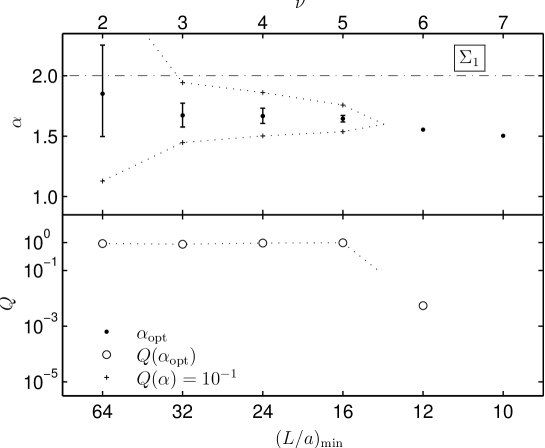
Figure 13: Fit A for the large $N$ data $\Sigma_{1}(u_{0},L)$ with artificial errors added.

We see a rather similar picture for this case where we are confident of the lattice artefacts really having the Symanzik form. Very similar plots can also be generated from the leading $N=\infty$ term. Also in Fig. 5 the new data points would resemble the structure exhibited by the Monte Carlo data.

4 Conclusions

In this work we have further investigated the scaling violations of the finite volume mass gap step scaling function of the O($N$) model at various $N$. The discretizations are restricted to the standard action. The behaviour at $N=3$ is confirmed by our added data and by our method of analysis. With fits of the form (6) a rather large number of coarser lattices has to be excluded, and then a cutoff dependence with an exponent $1<\alpha<2$ seems to be suggested in the accessible range of lattice spacings. With one additional logarithmic correction both exponents 1 (ad hoc) and 2 (Symanzik) (7,8) can be used with again only the finer lattices included. For $N=4,8$ a similar but less pronounced picture emerges. Our sensitivity is weaker since the lattice artefacts are generally much smaller and hence harder to measure. Although there may be a trend of ‘normalization’ with larger $N$, also at $N=4$ our data point toward $\alpha<2$ unless all lattices with $L/a<24$ are excluded.

It would be very interesting if theoretical principles could be found to organize a leading log summation of leading cutoff effects in analogy to the renormalization group improvement of continuum results. Such an attempt is here left to future study.

At $N=\infty$ it is rigorously known due to [12] that cutoff effects are of the Symanzik type with just $1/L^{2},\ln(L)/L^{2}$ contributions. The leading $1/N$ correction to the step scaling function, worked out here for the first time, somewhat to our surprise seems to have just the same behaviour, although this can be only demonstrated numerically at present. Needless to say, we cannot exclude other admixtures if they are only small enough. When these exact results are analyzed in the same way as the Monte Carlo data, a qualitatively similar picture emerges. It is hence very clear that we cannot conclude a truly anomalous scaling behavior from the latter.

The large $N$ sigma model proved to be a very interesting case, also because we here have an analytic handle on quantities that are nonperturbative in the coupling of an asymptotically free theory. This is true for both the continuum and at finite lattice spacing. This simplified laboratory can certainly be useful to study other issues.

Acknowledgements. We would like to thank Janos Balog, Burkhard Bunk, Tomasz Korzec and Peter Weisz for helpful discussions. This work was supported by the Deutsche Forschungsgemeinschaft in the form of Graduiertenkolleg GK 271 and Sonderforschungsbereich SFB TR 09.

References

- [1] K. Symanzik, Recent developments in gauge theories (Cargése, 1979), edited by G. ’t Hooft et. al., New York, 1980, Plenum Press.
- [2] U. Wolff, Phys. Rev. Lett. 62 (1989) 361.
- [3] M. Lüscher, P. Weisz and U. Wolff, Nucl. Phys. B359 (1991) 221.
- [4] M. Hasenbusch, Nucl. Phys. Proc. Suppl. 42 (1995) 764, hep-lat/9408019.
- [5] P. Hasenfratz and F. Niedermayer, Nucl. Phys. B596 (2001) 481, hep-lat/0006021.
- [6] M. Hasenbusch, P. Hasenfratz, F. Niedermayer, B. Seefeld and U. Wolff, Nucl. Phys. Proc. Suppl. 106 (2002) 911, hep-lat/0110202.
- [7] M. Lüscher, Phys. Lett. B118 (1982) 391.
-
[8]
B. Leder,
Nonstandard Cutoff Effects in Nonlinear Sigma
Models,
Master’s thesis, Mathematisch-Naturwissenschaftlichen
Fakultät I, Humboldt-Universität zu Berlin, 2003,
http://edoc.hu-berlin.de/abstract.php3?id=86000960. - [9] J. Balog and A. Hegedus, J. Phys. A37 (2004) 1881, hep-th/0309009.
- [10] J. Balog, private communication.
- [11] W.H. Press, S.A. Teukolsky, W.T. Vetterling and B.P. Flannery, Numerical Recipes, Fortran, 2nd ed. (Cambridge University Press, 1992).
- [12] S. Caracciolo and A. Pelissetto, Phys. Rev. D58 (1998) 105007, hep-lat/9804001.
- [13] H. Flyvbjerg and S. Varsted, Nucl. Phys. B344 (1990) 646.
- [14] P. Weisz, The universal z-z’ curve in the nonlinear -model in the limit , unpublished notes.
- [15] D.S. Shin, Nucl. Phys. B546 (1999) 669, hep-lat/9810025.
- [16] ALPHA, A. Bode et al., Phys. Lett. B515 (2001) 49, hep-lat/0105003.
- [17] M. Lüscher and P. Weisz, Nucl. Phys. B266 (1986) 309.
- [18] J. Balog and U. Wolff, work in progress.