DESY 05-082

HU-EP-05/22

SFB/CPP-05-19

On lattice actions for static quarks

Michele Della Morte^a, Andrea Shindler^b and Rainer Sommer^c
a Institut für Physik, Humboldt Universität,

Newtonstr. 15, 12489 Berlin, Germany ^b NIC/DESY,

Platanenallee 6, 15738 Zeuthen, Germany ^c DESY,

Platanenallee 6, 15738 Zeuthen, Germany
Abstract

We introduce new discretizations of the action for static quarks. They achieve an exponential improvement (compared to the Eichten-Hill regularization) on the signal to noise ratio in static–light correlation functions. This is explicitly checked in a quenched simulation and it is understood quantitatively in terms of the self energy of a static quark and the lattice heavy quark potential at zero distance. We perform a set of scaling tests in the Schrödinger functional and find scaling violations in the O($a$) improved theory to be rather small – for one observable significantly smaller than with the Eichten-Hill regularization. In addition we compute the improvement coefficients of the static light axial current up to ${\rm O}(g_{0}^{4})$ corrections and the corresponding renormalization constants non-perturbatively. The regularization dependent part of the renormalization of the b-quark mass in static approximation is also determined. Key words: Lattice QCD; Heavy quark effective theory; Static approximation; Non-perturbative renormalization PACS: 11.10.Gh; 11.15.Ha; 12.38.Gc; 13.20.He

June 2005

1 Introduction

Lattice QCD is playing an important rôle in the interpretation of B-physics experiments [?]. However, as new physics is hiding behind the standard model, the required precision for lattice computations of B-meson transition amplitudes is becoming more and more demanding. The development of new algorithms [?,?,?,?] promises that light dynamical fermions at small lattice spacings, $a$, can be reached in the near future, which will reduce one of the most important systematic errors.

Still, the treatment of b-quarks on the lattice remains another difficult part of these computations, since it appears unlikely that lattice spacings small enough to satisfy $a<1/m_{{\rm b}}$ will soon come into reach. We refer the reader to reviews for an explanation of the various approaches to this problem [?,?,?].

A theoretically clean solution is provided by HQET. This effective theory starts from the static approximation describing the asymptotics as $m_{{\rm b}}\to\infty$. Corrections ${\rm O}(1/m_{{\rm b}})$ have to be computed by a $1/m_{{\rm b}}$ expansion, where the higher dimensional interaction terms in the effective Lagrangian are treated as insertions into static correlation functions. An attractive feature of this approach is that the continuum limit exists and results are independent of the regularization. The theory requires non-perturbative renormalization, but a concrete way to carry this out has been proposed and tested for a simple case [?].

Furthermore also just the leading order term (static) is of considerable interest, since it provides a limit of the theory, which in many cases is not expected to be far from results at the physical point. Other methods to treat heavy quarks can thus be tested by checking whether they smoothly approach the static limit $1/m_{{\rm b}}\to 0$. In fact, results can also be obtained from interpolations in $1/m_{{\rm b}}$ between points below the b-quark mass and the static limit, see [?] for a precise demonstration.

As we will discuss in detail in section 2.1, the noise-to-signal ratio of static-light correlation functions grows exponentially in Euclidean time, $\sim\exp(\mu x_{0})$ and the rate $\mu\sim 1/a$ diverges as one approaches the continuum limit. Good statistical precision is difficult to reach for $x_{0}>1\,{\rm fm}$ [?,?]. In the past, sophisticated wavefunction techniques have been used to obtain ground state properties [?,?,?]. The results of these attempts, obtained with the standard Eichten-Hill regularization [?], were not completely satisfactory in all cases [?]. In [?] we used the fact that $\mu$ is not universal. By changing the regularization, we were able to obtain results at large $x_{0}$, where the ground state can be isolated with good statistical and systematic precision. Here we will discuss these alternative actions in more details. Particular emphasis is put on the size of discretization errors, since their smallness should always be the first criterion for choosing an action. Let us mention right away that we will consider only actions, which share the symmetries, eqs. (2.18,2.19), with the Eichten-Hill action, since these guarantee that no ${\rm O}(a)$ terms are needed in the static action to have ${\rm O}(a)$ improvement. For all actions considered, we determine the coefficients of the improvement terms needed for the axial current with 1-loop precision. In particular we correct for a mistake in the perturbative computation of the improvement coefficients in [?], see the Erratum. Furthermore we determine the action-dependent parts of the renormalization of the static axial current and the b-quark mass.

Before coming to the description of the static actions, we list some preliminaries. As a probe of the theory, we will consider correlation functions defined by the Schrödinger functional (SF) [?,?]. For the introduction of static quarks in the SF as well as any unexplained notation we refer to [?]. We adopted the ${\rm O}(a)$-improved Wilson regularization [?,?] with non-perturbatively determined value of $c_{\rm SW}$ [?] for the light quarks. The gauge sector is discretized through the Wilson plaquette action.

Below we will report also on results of Monte Carlo computations. Our simulation parameters are summarized in appendix C. All the results have been obtained in the quenched approximation, a part of them already appeared in [?] and [?].

2 Static actions

Static quarks are introduced on the lattice through fermionic fields $\psi_{\rm h}$ and $\overline{\psi}_{\rm h}$, which live on the lattice sites and satisfy the projection properties

$$P_{+}\psi_{\rm h}=\psi_{\rm h}\;,\quad\quad\overline{\psi}_{\rm h}P_{+}=\overline{\psi}_{\rm h}\;,\quad\quad P_{+}={{1+\gamma_{0}}\over{2}}\;.$$ (2.1)

The action $S_{\rm h}$ for static quarks has been derived by Eichten and Hill in [?]. Here we adopt a notation, which allows us to provide a generalization of that action and write it in the form

$$S_{\rm h}^{\rm W}=a^{4}{{1}\over{1+a\;\delta m_{\rm W}}}\sum_{x}\overline{\psi}_{\rm h}(x)(D_{0}^{\rm W}+\delta m_{\rm W})\psi_{\rm h}(x)\;,$$ (2.2)

with the covariant derivative

$$D_{0}^{\rm W}\psi_{\rm h}(x)={{1}\over{a}}\left[\psi_{\rm h}(x)-W^{\dagger}(x-a\hat{0},0)\psi_{\rm h}(x-a\hat{0})\right]\;,$$ (2.3)

where $W(x,0)$ is a gauge parallel transporter with the gauge transformation properties of the link $U(x,0)$. The Eichten-Hill action is given by setting $W(x,0)=U(x,0)$. The quark propagator $G_{\rm h}^{\rm W}(x,y)$ satisfying $(D_{0}^{\rm W}+\delta m_{\rm W})G_{\rm h}^{\rm W}(x,y)=\delta(x-y)P_{+}$, reads

$$\!\!\!\!\!\!\!\!\!\!\!\!\!G_{\rm h}^{\rm W}(x,y) \!\!\!=\!\!\! \theta(x_{0}-y_{0})\;\delta({\bf{x-y}})\;(1+a\;\delta m_{\rm W})^{-(x_{0}-y_{0})/a}\;{\cal{P}}^{\rm W}(y,x)^{\dagger}\;P_{+}\;,$$ (2.4)

$$\!\!\!\!\!\!\!\!\!\!\!\!\!{\cal{P}}^{\rm W}(x,x) \!\!\!=\!\!\! 1\;,$$ (2.5)

$$\!\!\!\!\!\!\!\!\!\!\!\!\!{\cal{P}}^{\rm W}(x,x+R\hat{\mu}) \!\!\!=\!\!\! W(x,\mu)W(x+a\hat{\mu},\mu)\dots W(x+a(R-1)\hat{\mu},\mu)\;\;{\rm for\;\;R>0},$$ (2.6)

where $\delta m_{\rm W}$ cancels the divergence in the self-energy of the static quark (see below).

2.1 Noise to signal ratio

In order to simplify the following discussion we start from the action in eq. (2.2) but set $\delta m_{\rm W}=0$. This is possible since the dependence of correlation functions on $\delta m_{\rm W}$ is known exactly from the form of the static quark propagator in eqs. (2.4-2.6) and can be restored easily. The noise to signal ratio discussed here is independent of $\delta m_{\rm W}$. As an example we consider a correlation function of heavy-light fields such as $f_{\rm A}^{\rm stat}(x_{0})$, which describes the propagation of a static–light pseudoscalar meson. Its definition

$$f_{\rm A}^{\rm stat}(x_{0})=-{{a^{6}}\over{2}}\sum_{{\bf y},{\bf z}}\langle A_{0}^{\rm stat}(x)\overline{\zeta}_{\rm h}({\bf y})\gamma_{5}\zeta_{\rm l}({\bf z})\rangle\;,$$ (2.7)

involves the boundary fields $\overline{\zeta}_{\rm h}$ and $\zeta_{\rm l}$ (see [?]) as well as the time component of the axial current

$$A_{0}^{\rm stat}(x)=\overline{\psi}_{\rm l}(x)\gamma_{0}\gamma_{5}\psi_{\rm h}(x)\;,$$ (2.8)

where the subscript ‘l’ indicates the light quark fields. The correlation function is represented pictorially in figure 1.

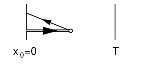
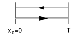
Figure 1: Schematic representation of the correlation functions $f_{\rm A}^{\rm stat}(x_{0})$ and $f_{1}^{\rm stat}$ in the SF. The double lines indicate the static quark propagators.

From the quantum mechanical representation one expects the large $x_{0}$ asymptotic behavior

$$f_{\rm A}^{\rm stat}(x_{0})\propto e^{-E_{\rm stat}x_{0}}\;,$$ (2.9)

where $E_{\rm stat}$ is the binding energy of the static–light system. It depends on the choice for $W$ and diverges approximately linearly in the lattice spacing.

$$E_{\rm stat}\sim E_{\rm self}+{\rm O}(a^{0})\sim{{1}\over{a}}e^{(1)}\;g_{0}^{2}+\dots\;.$$ (2.10)

This divergence is to be canceled by $\delta m_{\rm W}=-E_{\rm self}+{\rm O}(a^{0})$. The finite part of $\delta m_{\rm W}$ is of course scheme dependent, but in perturbation theory one can always perform the double expansion

$$E_{\rm self} = E_{\rm self}^{(1)}\,g_{0}^{2}+{\rm O}(g_{0}^{4})\,,$$ (2.11)

$$E_{\rm self}^{(1)} = {{1}\over{a}}e^{(1)}+{\rm O}(a^{0})\,.$$ (2.12)

For example, if we define $E_{\rm self}$ from a Schrödinger functional correlation function (see eq. (A.76)), the $a$-expansion appears as an expansion in terms of $a/L$. The coefficient $e^{(1)}$ does then depend on the action, but not on the correlation function used to define it.

We now want to discuss the noise to signal ratio of the Monte Carlo estimate of $f_{\rm A}^{\rm stat}$. The variance of a generic observable $\cal O$ in a QCD simulation is given by $\langle\tilde{\cal O}^{2}\rangle_{\rm G}-\langle\tilde{\cal O}\rangle_{\rm G}^{2}$, where the expectation value $\langle...\rangle_{\rm G}$ is an average over the gauge fields including the weight obtained after integrating out the fermion fields (the fermion determinant). $\tilde{\cal O}$ is derived from $\cal O$ by performing the corresponding Wick contractions on each gauge field background. In the Monte Carlo one takes advantage of translation invariance on the r.h.s. of eq. (2.7) and estimates $f_{\rm A}^{\rm stat}=\langle\cal O\rangle$ with ${\cal O}=-{{a^{9}}\over{2L^{3}}}\sum_{{\bf y},{\bf z},{\it\bf x}}A_{0}^{\rm stat}(x)\overline{\zeta}_{\rm h}({\bf y})\gamma_{5}\zeta_{\rm l}({\bf z})$. Its variance, $\sigma_{\rm A}(x_{0})$, can be rewritten as

$$\sigma_{\rm A}(x_{0}) = {{a^{18}}\over{4L^{6}}}\sum_{{\bf x,y,z,x^{\prime},y^{\prime},z^{\prime}}}\left\langle\,[A_{0}^{\rm stat}]_{\rm hl}(x_{0},{\it\bf x})\,\overline{\zeta}_{\rm h}({\bf y})\gamma_{5}\zeta_{\rm l}({\bf z})\times\right.$$ (2.13)

$$\left.\qquad\left\{[A_{0}^{\rm stat}]_{\rm h^{\prime}l^{\prime}}(x_{0},{\it\bf x}^{\prime})\,\overline{\zeta}_{\rm h^{\prime}}({\bf y^{\prime}})\gamma_{5}\zeta_{\rm l^{\prime}}({\bf z^{\prime}})\right\}^{\dagger}\,\right\rangle\;-\;[f_{\rm A}^{\rm stat}(x_{0})]^{2}\,,$$

where $\rm h^{\prime}$ and $\rm l^{\prime}$ denote copies of $\rm h$ and $\rm l$ differing only by their flavor, which are introduced to be able to write the variance in the form of a standard expectation value. Saturating $\sigma_{\rm A}(x_{0})$ with intermediate states shows that its large $x_{0}$ asymptotics is

$$\sigma_{\rm A}(x_{0})\propto\sum_{\bf x,x^{\prime}}\,C({\it\bf x},{\it\bf x}^{\prime})\,{\rm e}^{-x_{0}E_{\rm ll^{\prime}}({\it\bf x},{\it\bf x}^{\prime})}\,,$$ (2.14)

with $E_{\rm ll^{\prime}}({\it\bf x},{\it\bf x}^{\prime})$ the energy of a state with a static quark-antiquark pair at positions ${\it\bf x},{\it\bf x}^{\prime}$ and a light quark-antiquark pair with flavors $\rm l,l^{\prime}$. At large $x_{0}$ the sum is dominated by the term with the smallest energy $E$. This is expected to be given by ${\it\bf x}={\it\bf x}^{\prime}$, where the color charges of the static quark and anti-quark compensate. The light quark-antiquark pair should then feel little of the static quarks and its lowest energy be given approximately by $m_{\pi}$. This argument suggests

$${\rm Min}_{{\it\bf x},{\it\bf x}^{\prime}}\,E_{\rm ll^{\prime}}({\it\bf x},{\it\bf x}^{\prime})=V(0)+m_{\pi}\,.$$ (2.15)

Here $V(0)$ is the lattice static quark potential at zero distance, which for example is computable via the large $x_{0}$ asymptotics

$$\langle\,\overline{\psi}_{\rm h}(x)\gamma_{5}\psi_{\rm h^{\prime}}(x)\,\overline{\zeta}_{\rm h^{\prime}}({{\it\bf x}})\gamma_{5}\zeta_{\rm h}({{\it\bf x}})\,\rangle\propto{\rm e}^{-x_{0}V(0)}\,.$$ (2.16)

The noise to signal ratio $R_{\rm NS}$ for $f_{\rm A}^{\rm stat}(x_{0})$ should then approach

$$R_{\rm NS}\propto e^{[E_{\rm stat}-(m_{\pi}+V(0))/2]\,x_{0}}\;.$$ (2.17)

For the Eichten-Hill action (or more generally whenever $W(x,0)$ is unitary), the lattice potential vanishes at zero distance and one obtains the formula given earlier by Lepage [?]. We infer from eq. (2.17) that the linear divergence in $E_{\rm stat}$ is responsible for the exponential growth of the error with the Euclidean time $x_{0}$, which has been observed in many numerical investigations of correlation functions such as $f_{\rm A}^{\rm stat}$ [?,?,?,?]. It is then clear that the problem becomes more severe as the continuum limit is approached. In particular, for the Eichten-Hill action the coefficient $e^{(1)}$ was found to be rather large [?] rendering precise computations hopeless. Finally we remark again that the form of the static propagator shows that $R_{\rm NS}$ is (exactly) independent of $\delta m_{\rm W}$. In the final formula eq. (2.17) this is realized since $E_{\rm stat}$ and $V(0)/2$ are shifted by the same amount,

$$\left.aE_{\rm stat}\right|_{\delta m_{\rm W}} = \left.aE_{\rm stat}\right|_{\delta m_{\rm W}=0}+\ln(1+a\delta m_{\rm W})$$

$$\left.aV(0)\right|_{\delta m_{\rm W}} = \left.aV(0)\right|_{\delta m_{\rm W}=0}+2\ln(1+a\delta m_{\rm W}).$$

2.2 Statistically improved discretizations

A possible way to improve on the problem discussed in the previous section is to employ actions $S_{\rm h}^{W}$ inspired by variance reduction methods. Such methods led for example to the introduction of the one-link integral (or multihit) [?] in the pure gauge theory. This provides unbiased estimators for quantities such as Polyakov loop correlation functions, significantly reducing at the same time their variance. Here, a similar change will not lead to an unbiased estimator, but rather has to be considered a change of the static action. Alternatively (or simultaneously) one can try to enhance the signal by choosing the parallel transporter $W$ such that $E_{\rm stat}\sim E_{\rm self}$ is comparatively small (assuming $V(0)$ to be numerically less relevant). In addition to this, we want to preserve on the lattice the following symmetries of the static theory

• Heavy quark spin symmetry:

  $$\psi_{\rm h}\longrightarrow{\cal V}\psi_{\rm h}\,,\qquad\overline{\psi}_{\rm h}\longrightarrow\overline{\psi}_{\rm h}{\cal V}^{-1}\,,\quad{\rm with}\quad{\cal V}=\exp(-i\phi_{i}\epsilon_{ijk}\sigma_{jk})\,,$$ (2.18)

• Local conservation of heavy quark flavor number:

  $$\psi_{\rm h}\longrightarrow{\rm e}^{i\eta({\it\bf x})}\,\psi_{\rm h},\qquad\overline{\psi}_{\rm h}\longrightarrow\overline{\psi}_{\rm h}{\rm e}^{-i\eta({\it\bf x})}.$$ (2.19)

Together with gauge invariance, parity and cubic symmetry, this is enough to guarantee that the universality class and the O($a$) improvement are unchanged with respect to the Eichten-Hill action, as has been discussed in [?]. Furthermore we want to keep the action as local as possible. We therefore exclude constructions of $W$ which involve fields at a distance two lattice spacings or more away from the link $U(x,0)$. Taking these considerations into account, we propose the following regularized actions

$$S_{\rm h}^{\rm A} :\quad W^{\rm A}(x,0)= V(x,0)\;,$$ (2.20)

$$S_{\rm h}^{\rm s} :\quad W^{\rm s}(x,0)= V(x,0)\left[{{g_{0}^{2}}\over{5}}+\left({{1}\over{3}}\,\hbox{tr}\,V^{\dagger}(x,0)V(x,0)\right)^{1/2}\right]^{-1}\;,$$ (2.21)

$$S_{\rm h}^{\rm HYP} :\quad W^{\rm HYP}(x,0)= V_{\rm HYP}(x,0)\;,$$ (2.22)

where $V(x,0)$ is the average of the six staples around the link $U(x,0)$

$$V(x,0) = {{1}\over{6}}\sum_{j=1}^{3}\left[U(x,j)U(x+a\hat{j},0)U^{\dagger}(x+a\hat{0},j)\right.$$ (2.23)

$$\qquad\;\left.+U^{\dagger}(x-a\hat{j},j)U(x-a\hat{j},0)U(x+a\hat{0}-a\hat{j},j)\right]\;,$$

and $V_{\rm HYP}$ is the HYP link [?]. In the latter case three coefficients $(\alpha_{1},\alpha_{2},\alpha_{3})\;\equiv\vec{\alpha}$ need to be specified in order to define the combination of differently smeared links in the construction of the HYP link. In the following we will only discuss the choices $\vec{\alpha}=(0.75,0.6,0.3)$, motivated in [?] and $\vec{\alpha}=(1.0,1.0,0.5)$ obtained by an approximate minimization of $R_{\rm NS}$. They define $S_{\rm h}^{\rm HYP1}$ and $S_{\rm h}^{\rm HYP2}$ respectively. The construction of HYP links involves projecting $3\times 3$ complex matrices onto SU(3). As we expect deviations from SU(3) to be small, we prefer approximating the projection by an analytic function defined by the steps

$$W\rightarrow{{W}\,/\,{\sqrt{\,\hbox{tr}\,(WW^{\dagger})/3}}}\;,$$ (2.24)

followed by 4 iterations of

$$W\rightarrow X\left(1-\hbox{$\rm i\over 3$}{\rm Im}\,\left(\det X\right)\right)\;,\quad{\rm with}\quad X=W\left(\hbox{$3\over 2$}-\hbox{$1\over 2$}W^{\dagger}W\right)\;.$$ (2.25)

To be precise, this function is to be taken as part of the definition of $V_{\rm HYP}$, when our numerical results for improvement coefficients and renormalization factors are used in subsequent computations.

For the actions $S_{\rm h}^{\rm HYP1}$ and $S_{\rm h}^{\rm HYP2}$ the value of $e^{(1)}$ has been computed in [?]. In the cases $W\in\!\!\!\!\!/$ SU(3) it is more convenient to look at $E_{\rm self}-V(0)/2$ not only because this is the relevant quantity for the noise to signal ratio, but also because at 1-loop order the deviations of the links $W$ from unitarity cancel in the combination. We indicate by $r^{(1)}$ the 1-loop coefficient in the perturbative expansion

$$E_{\rm self}-V(0)/2\sim\left({{1}\over{a}}r^{(1)}+{\rm O}(a^{0})\right)\;g_{0}^{2}+{\rm O}(g_{0}^{4})\;.$$ (2.26)

Of course $r^{(1)}=e^{(1)}$ for $S_{\rm h}^{\rm HYP}$ and $S_{\rm h}^{\rm EH}$. In appendix A we outline a computation of $r^{(1)}$ for $S_{\rm h}^{\rm A}$ and explain why it is the same for $S_{\rm h}^{\rm s}$ (at one-loop order).

$S_{\rm h}^{\rm W}$	$r^{(1)}$	$aE_{\rm stat}$	$aV(0)$
$S_{\rm h}^{\rm EH}$	0.16845(2)	0.68(9)	0.0
$S_{\rm h}^{\rm A}$	0.05737(4)	0.85(2)	0.671(2)
$S_{\rm h}^{\rm s}$	0.05737(4)	0.76(2)	0.496(2)
$S_{\rm h}^{\rm HYP1}$	0.04844(1)	0.44(2)	0.0
$S_{\rm h}^{\rm HYP2}$	0.03523(1)	0.41(1)	0.00001(1)

Table 1: One loop coefficients $r^{(1)}$, defined in eq. (2.26) and non-perturbative values for $aE_{\rm stat}$ and $aV(0)$ at $\beta=6$.

Some results for $r^{(1)}$ are collected in table 1. From the table we see that perturbation theory already suggests $S_{\rm h}^{\rm HYP2}$ as the most favorable choice concerning signal enhancement.

The discretizations $S_{\rm h}^{\rm A}$ and $S_{\rm h}^{\rm s}$ are inspired by noise reduction methods, namely APE smearing and one-link integral respectively. APE smearing was introduced in [?] where it was shown to suppress fluctuations in gauge invariant quantities in the pure gauge theory. As shown by $r^{(1)}$, this can also be interpreted as a reduction of the static self energy. Finally $W^{\rm s}$ is an approximation of the SU(3) one-link integral. For completeness we describe briefly how we arrived at $S_{\rm h}^{\rm s}$ in appendix B. The reader may, however, take it just as another ansatz satisfying our criteria explained above.

The effectiveness of these regularizations in reducing the noise to signal ratio in static–light correlation functions has been checked non-perturbatively by a simulation on a $16^{3}\times 32$ lattice at $\beta=6/g_{0}^{2}=6$, where the lattice spacing is $a\approx\,0.1\,{\rm fm}$ (the hopping parameter $\kappa$ has been set to the strange quark mass value, $\kappa=0.133929$, as in [?]). Figure 2 shows the results for $R_{\rm NS}$ obtained using an ensemble of almost 5000 configurations.

Figure 2: The ratio $R_{\rm NS}$ for the correlation function $f_{\rm A}^{\rm stat}(x_{0})$ for a statistics of 5000 measurements on a $16^{3}\times 32$ lattice at $\beta=6$. Filled circles refer to $S_{\rm h}^{\rm EH}$, empty circles to $S_{\rm h}^{\rm A}$ ($S_{\rm h}^{\rm s}$ gives similar results), empty (filled) triangles to $S_{\rm h}^{\rm HYP1}$ ($S_{\rm h}^{\rm HYP2}$).

The largest improvement is again given by the action $S_{\rm h}^{\rm HYP2}$, but we see from the figure that all the proposed discretizations produce a clear signal (for the considered statistics) at least up to a time separation of roughly $2\;{\rm fm}$. The dotted lines in figure 2 represent the predictions from eq. (2.17), where for $aE_{\rm stat}$, $aV(0)$ and $am_{\pi}$ we insert the estimates from the data. We summarize the obtained values of $aE_{\rm stat}$ and $aV(0)$ in table 1. The formula in eq. (2.17) turns out to be always quite accurate in describing the results. Furthermore, assuming $E_{\rm stat}-V(0)/2$ to be dominated by its divergent term and approximating it by the leading perturbative estimate yields the correct order for $R_{\rm NS}$. It is thus to be expected that the ordering of $R_{\rm NS}$ observed in figure 2 will be preserved when going to smaller lattice spacings, where it is even more important to keep $R_{\rm NS}$ at a reasonable level if one wants to reach distances $x_{0}$ around $1-2$ fm. Indeed, numerical experience supports this expectation [?].

3 The size of discretization errors

In addition to the reduction of statistical errors, the size of scaling violations has to be taken into account when one chooses between different actions. For this reason we designed a number of scaling tests by which we could study the approach of a set of quantities defined in the SF to their continuum limit values. Before going into the details of this study we first need to discuss the computation of the O($a$) improvement coefficients of the static axial current for the different actions introduced.

3.1 Computation of the improvement coefficients $c_{\rm A}^{\rm stat}$ and $b_{\rm A}^{\rm stat}$

The O($a$) improvement programme [?,?] has been carried out for the EH action in [?]. In [?] the discussion has been extended to the actions we are considering here. As mentioned in the previous section, arguments based on the symmetries preserved on the lattice allow to show that the improvement pattern is the same in all cases. In particular the actions are improved once the light sector has been improved; no new improvement terms are needed for the static part of the actions.

Concerning the static–light axial density $A_{0}^{\rm stat}(x)$, the improved version reads

$$(A^{\rm stat}_{\rm I})_{0}\!=\!A^{\rm stat}_{0}(x)\!+\!ac_{\rm A}^{\rm stat}\delta A^{\rm stat}_{0}(x)\;,\quad\delta A^{\rm stat}_{0}(x)\!=\!\overline{\psi}_{\rm l}(x)\gamma_{j}\gamma_{5}\!{{\overleftarrow{\nabla}_{j}}\!+\!\overleftarrow{\nabla}\kern-0.5pt\smash{\raise 4.5pt\hbox{$\ast$}}\kern-4.5pt_{j}\over 2}\psi_{\rm h}(x)\;,$$ (3.27)

where the improvement coefficient $c_{\rm A}^{\rm stat}$ has been introduced. In a mass independent renormalization scheme the renormalized density can be written

$$(A_{\rm R}^{\rm stat})_{0}=Z_{\rm A}^{\rm stat}(g_{0},a\mu)(1+b_{\rm A}^{\rm stat}am_{\rm q})(A^{\rm stat}_{\rm I})_{0}\;,$$ (3.28)

with $m_{\rm q}$ the bare subtracted light quark mass (cf. eq. (C.104)), $Z_{\rm A}^{\rm stat}(g_{0},a\mu)$ the scale dependent renormalization factor of the axial current and $b_{\rm A}^{\rm stat}$ a second improvement coefficient. The values of $c_{\rm A}^{\rm stat}$ and $b_{\rm A}^{\rm stat}$, as well as $Z_{\rm A}^{\rm stat}$, depend on the choice for the static action. For the EH action the improvement coefficients $c_{\rm A}^{\rm stat}$ and $b_{\rm A}^{\rm stat}$ have been determined at 1-loop order of perturbation theory in [?,?,?], while the renormalization constant $Z_{\rm A}^{\rm stat}$ has been computed non-perturbatively in the SF scheme in [?]. In the remainder of this section we describe our computation of the improvement coefficients $c_{\rm A}^{\rm stat}$ and $b_{\rm A}^{\rm stat}$ for the actions in eqs. (2.20 - 2.22), and we present a set of scaling studies. We will come back to the renormalization constant $Z_{\rm A}^{\rm stat}$ in section 4, where we also discuss the improvement the new actions can bring in the computation of the b-quark mass following the strategy in [?,?].

3.1.1 Improvement conditions and results for $c_{\rm A}^{\rm stat}$ and $b_{\rm A}^{\rm stat}$

We want to compute the 1-loop coefficients $c_{\rm A}^{\rm stat,(1)}$ and $b_{\rm A}^{\rm stat,(1)}$ of the improvement constants $c_{\rm A}^{\rm stat}$ and $b_{\rm A}^{\rm stat}$. To this end we have adopted a mixed strategy. For $S_{\rm h}^{\rm A}$ and $S_{\rm h}^{\rm s}$ the computation has been carried out analytically, while for $S_{\rm h}^{\rm HYP1}$ and $S_{\rm h}^{\rm HYP2}$ we have used Monte Carlo simulations to numerically estimate an effective 1-loop coefficient for the coupling range relevant here. In both cases we have exploited the same improvement conditions. We collect some details of the analytic computation in appendix A.

We introduce the correlation $f_{\rm A,I}^{\rm stat}$ defined as $f_{\rm A}^{\rm stat}$ in eq. (2.7) with the current $A_{0}^{\rm stat}$ replaced by the improved current in eq. (3.27). Assuming the knowledge of $c_{\rm A}^{\rm stat}$ for a discretized action $S_{\rm h}^{1}$, we have enforced the condition

$${\left.f_{\rm A,I}^{\rm stat}(T/2,S_{\rm h}^{1})\right|_{\theta}\over\left.f_{\rm A,I}^{\rm stat}(T/2,S_{\rm h}^{1})\right|_{\theta^{\prime}}}\,=\,{\left.f_{\rm A,I}^{\rm stat}(T/2,S_{\rm h}^{2})\right|_{\theta}\over\left.f_{\rm A,I}^{\rm stat}(T/2,S_{\rm h}^{2})\right|_{\theta^{\prime}}}\;,\quad\theta=0,\;\theta^{\prime}=1\;,\quad m_{\rm q}=0\;,$$ (3.29)

and solved the implicit relation for $c_{\rm A}^{\rm stat}$ of $S_{\rm h}^{2}$. Expanding eq. (3.29) in powers of the coupling $g_{0}^{2}$ and setting $S_{\rm h}^{1}=S_{\rm h}^{\rm EH}$, for which $c_{\rm A}^{\rm stat,(1)}$ is known from [?], we obtain

$$c_{\rm A}^{\rm stat}=c_{\rm A}^{\rm stat,(1)}\,g_{0}^{2}+{\rm O}(g_{0}^{4})\,,\quad c_{\rm A}^{\rm stat,(1)}=0.0072(4)\,,\quad\;\,{\rm for}\;S_{\rm h}^{\rm s}\;{\rm and}\;S_{\rm h}^{\rm A}\;.$$ (3.30)

The ratios in eq. (3.29) have then been evaluated, with $S_{\rm h}^{1}=S_{\rm h}^{\rm A}$, on the configurations generated in runs I to IV of table 6 in order to obtain $c_{\rm A}^{\rm stat}$ for $S_{\rm h}^{2}=S_{\rm h}^{\rm HYP1},\;S_{\rm h}^{\rm HYP2}$. There the size $L/a$ and the $\beta$ values have been chosen such that $L$ is kept fixed to $1.436r_{0}$ with $r_{0}$ from [?,?]. Our results are shown in figure 3.

Figure 3: Numerical results for the improvement coefficient $c_{\rm A}^{\rm stat}$. For $S_{\rm h}^{\rm EH}$ the result of [?] is plotted, for $S_{\rm h}^{\rm s}$ the band represents the result eq. (3.30), while otherwise it refers to the numerical estimates eqs. (3.31, 3.32).

The result for $S_{\rm h}^{\rm s}$ provides a test of the numerical procedure since it is known analytically (eq. (3.30)). We see that by ascribing to the numerical result an error, which covers the spread of the points we find agreement with eq. (3.30). This suggests that here higher orders in $g_{0}^{2}$ contribute little to the cutoff effects of the ratios appearing in eq. (3.29). We estimate in the same way the errors for $c_{\rm A}^{\rm stat}$ of $S_{\rm h}^{\rm HYP1}$ and $S_{\rm h}^{\rm HYP2}$, quoting the result

$$c_{\rm A}^{\rm stat}\approx 0.039(4)\,g_{0}^{2}\,,\quad\;\;{\rm for}\;S_{\rm h}^{\rm HYP1}$$ (3.31)

$$c_{\rm A}^{\rm stat}\approx 0.220(14)\,g_{0}^{2}\,,\quad{\rm for}\;S_{\rm h}^{\rm HYP2}\;.$$ (3.32)

Here the statistical errors are not the relevant ones. Rather our dominant error is due to the assumption (tested to some extent as just explained) that the 1-loop value for $c_{\rm A}^{\rm stat}$ for action $S_{\rm h}^{1}=S_{\rm h}^{\rm A}$ is accurate for our values of $g_{0}^{2}$. Apart from this, our determinations do provide a non-perturbative computation of $c_{\rm A}^{\rm stat}$ for the other actions. Thus the errors quoted in eqs. (3.31,3.32) include a reasonable (but not necessarily a safe) estimate of the perturbative uncertainty.

Note that for $S_{\rm h}^{\rm HYP2}$ the improvement coefficient is considerably larger than for the other actions. This means that before improvement the linear $a$-effects are larger in this case and one might expect that this will be the case also for higher order $a$-effects. We will see below that this is however not born out of our non-perturbative results.

Sensitivity to the improvement coefficient $b_{\rm A}^{\rm stat}$ is achieved by exploiting the quark mass dependence of the correlation function $f_{\rm A,I}^{\rm stat}(x_{0})$. Again, supposing $b_{\rm A}^{\rm stat}$ be known for the action $S_{\rm h}^{1}$, we consider the improvement condition

$${\left.(1+ab_{\rm A}^{\rm stat}(S_{\rm h}^{1})m_{\rm q^{\prime}})f_{\rm A,I}^{\rm stat}(T/2,S_{\rm h}^{1})\right|_{m_{\rm q^{\prime}}}\over\left.(1+ab_{\rm A}^{\rm stat}(S_{\rm h}^{1})m_{\rm q})f_{\rm A,I}^{\rm stat}(T/2,S_{\rm h}^{1})\right|_{m_{\rm q}}}={\left.(1+ab_{\rm A}^{\rm stat}(S_{\rm h}^{2})m_{\rm q^{\prime}})f_{\rm A,I}^{\rm stat}(T/2,S_{\rm h}^{2})\right|_{m_{\rm q^{\prime}}}\over\left.(1+ab_{\rm A}^{\rm stat}(S_{\rm h}^{2})m_{\rm q})f_{\rm A,I}^{\rm stat}(T/2,S_{\rm h}^{2})\right|_{m_{\rm q}}}\;,$$ (3.33)

with $\theta=1$, and solve for $b_{\rm A}^{\rm stat}$ of $S_{\rm h}^{2}$.

In perturbation theory $b_{\rm A}^{\rm stat}$ has been computed to 1-loop order in [?] for the Eichten–Hill regularization. Similarly to what we did for $c_{\rm A}^{\rm stat}$, we have then analytically computed $b_{\rm A}^{\rm stat}$ for $S_{\rm h}^{\rm A}$, i.e. we have expanded eq. (3.33) in perturbation theory with $S_{\rm h}^{\rm 1}=S_{\rm h}^{\rm EH}$ and $S_{\rm h}^{\rm 2}=S_{\rm h}^{\rm A}$. In this computation we set $m_{\rm q}=0$ and, following [?], $m_{\rm q^{\prime}}$ such that $Lm_{\rm R^{\prime}}=0.24$, with $m_{\rm R^{\prime}}$ the quark mass renormalized at scale $\mu=1/L$ in the minimal subtraction scheme on the lattice. The result reads

$$b_{\rm A}^{\rm stat}=1/2+b_{\rm A}^{\rm stat,(1)}\,g_{0}^{2}+{\rm O}(g_{0}^{4})\,,\quad b_{\rm A}^{\rm stat,(1)}=0.033(7)\,,\quad\;\,{\rm for}\;S_{\rm h}^{\rm s}\;{\rm and}\;S_{\rm h}^{\rm A}\;.$$ (3.34)

Next we impose eq. (3.33) on the data sets I to IV in table 6. Here, both $\kappa$ values and $\theta=1$ are used, where the second $\kappa$ value was determined such that $Lm_{\rm R^{\prime}}=0.24$ in the SF-scheme at scale $\mu=1/(1.436r_{0})$. With $S_{\rm h}^{1}=S_{\rm h}^{\rm A}$, we obtain

$$b_{\rm A}^{\rm stat}\approx 1/2+0.078(8)\,g_{0}^{2}\,,\quad\;\;{\rm for}\;S_{\rm h}^{\rm HYP1}$$ (3.35)

$$b_{\rm A}^{\rm stat}\approx 1/2+0.259(13)\,g_{0}^{2}\,,\quad{\rm for}\;S_{\rm h}^{\rm HYP2}\;.$$ (3.36)

The errors have been estimated as in the case of $c_{\rm A}^{\rm stat}$. We show the numerical results in figure 4. Again the improvement coefficient turns out largest for $S_{\rm h}^{\rm HYP2}$.

Figure 4: Numerical results for the improvement coefficient $b_{\rm A}^{\rm stat}$, presented as in figure 3.

One comment is in order here. In the condition in eq. (3.33), O$(am_{\rm q})$-terms with coefficients $b_{\rm g}$ and $b_{\zeta_{\rm h}}$ [?] are neglected, while terms proportional to $b_{\zeta}$ (see [?]) drop out. Of course, $b_{\zeta_{\rm h}}$ is O($g_{0}^{4}N_{\rm f}$) and therefore irrelevant in a 1-loop computation. While $b_{g}$ is O$(g_{0}^{2}N_{\rm f})$, it enters expectation values only with an additional factor $g_{0}^{2}$ (unless there is a non-zero background gauge field). In other words, eq. (3.33) is correct up to ${\rm O}(g_{0}^{4})$ in full QCD, but in the quenched approximation it is valid also non-perturbatively.

3.2 Scaling tests

On the same set of configurations used for the determination of $c_{\rm A}^{\rm stat}$ and $b_{\rm A}^{\rm stat}$ (runs I–IV), and for $\kappa=\kappa_{\rm c}$, we have computed (for each regularization) the ratios

$$\xi_{\rm A}(\theta,\theta^{\prime})={{\left.f_{\rm A,I}^{\rm stat}(T/2)\right|_{\theta}}\over{\left.f_{\rm A,I}^{\rm stat}(T/2)\right|_{\theta^{\prime}}}}\;,\quad\xi_{1}(\theta,\theta^{\prime})={{\left.f_{1}^{\rm stat}\right|_{\theta}}\over{\left.f_{1}^{\rm stat}\right|_{\theta^{\prime}}}}\;,\quad h(d/L)={{f_{1}^{\rm hh}(d)}\over{f_{1}^{\rm hh}(L/2)}}\;.$$ (3.37)

Here and in the following $f_{\rm A,I}^{\rm stat}(x_{0})$ refers to the 1-loop improved axial current in eq. (3.27). The correlation function $f_{1}^{\rm stat}$ is schematically represented in the right part of figure 1, it precisely reads

$$f_{1}^{\rm stat}=-{{a^{12}}\over{2L^{6}}}\sum_{\bf u,v,y,z}\;\langle\overline{\zeta}_{\rm l}\kern 1.0pt^{\prime}({\bf u})\gamma_{5}\zeta_{\rm h}\kern 1.0pt^{\prime}({\bf v})\;\overline{\zeta}_{\rm h}({\bf y})\gamma_{5}\zeta_{\rm l}({\bf z})\rangle\;,$$ (3.38)

with the primed fields living on the boundary at $x_{0}=T$. The quantity $h(d/L)$ was introduced in [?]. It is defined through the boundary to boundary SF correlator

$$f_{1}^{\rm hh}(x_{3})=-{{a^{8}}\over{2L^{2}}}\sum_{x_{1},x_{2},{\bf y},{\bf z}}\;\langle\overline{\zeta}_{\rm h}\kern 1.0pt^{\prime}({\bf x})\gamma_{5}\zeta_{\rm h}\kern 1.0pt^{\prime}({\bf 0})\;\overline{\zeta}_{\rm h}({\bf y})\gamma_{5}{\zeta_{\rm h}}({\bf z})\rangle\;,$$ (3.39)

note that the sum runs on $x_{1}$ and $x_{2}$ and therefore yields an $x_{3}$-dependent correlation function.

All the quantities in eq. (3.37) have a finite continuum limit in a fixed, finite, volume. The continuum result is universal, but the way it is approached depends on the details of the regularization. The scaling of these ratios can then provide an idea about the size of discretization effects for the static actions in eqs. (2.20 - 2.22). Our results are shown in figure 5.

Figure 5: Scaling plots for $\xi_{\rm A}(0,0.5)$, $\xi_{1}(0,0.5)$ and $h(1/4)$. Symbols are as in figure 2, some of them have been shifted on the horizontal axis for clarity. Again the results for $S_{\rm h}^{\rm s}$ are similar to the ones from $S_{\rm h}^{\rm A}$ and haven’t been plotted.

The cutoff effects in $\xi_{\rm A}$ are somewhat larger with the Eichten–Hill action than with any of our alternatives. Still, it is more relevant to note that all cutoff effects visible in the figure are very small and linear in $a^{2}$. This suggests that the O($a$) improvement programme has been implemented in a satisfactory way for the lattice spacings considered here – also for $S_{\rm h}^{\rm HYP2}$, where the improvement coefficients turn out to be not that small.

The gain in statistical precision brought by the new discretizations of the static action can also be seen in figure 5, especially for the quantity $h(1/4)$, which involves two static quarks propagating over the whole temporal extent.

Another interesting observable is the step scaling function introduced in [?] for the renormalization of the b-quark mass and further discussed in the following section. Here we simply define it as

$$\Sigma_{\rm m}(u,a/L) = 2L\left[\Gamma_{\rm stat}(2L)-\Gamma_{\rm stat}(L)\right]_{u=\bar{g}^{2}(L)}\;$$ (3.40)

$$\Gamma_{\rm stat}(L) = {{1}\over{2a}}\ln\left[f_{\rm A,I}^{\rm stat}(x_{0}-a)/f_{\rm A,I}^{\rm stat}(x_{0}+a)\right]\;,\quad\theta=1/2\,,\;T=L\,,$$ (3.41)

in terms of the correlation function $f_{\rm A,I}^{\rm stat}$ and the Schrödinger functional coupling $\bar{g}(L)$ [?,?,?], which fixes the length scale $L$. The continuum limit of $\Sigma_{\rm m}$ is, for each value of the coupling $u$, a universal quantity, independent of the regularization used. The step scaling function can hence be used for a further scaling study, in particular since discretization errors with the EH action turn out to be clearly visible [?]. Figure 6 shows that they are rather linear in $(a/L)^{2}$ for all actions considered. Compared to the EH action, the alternative ones show smaller lattice artefacts. In fact they are the smallest for $S_{\rm h}^{\rm HYP2}$ which also showed the best noise to signal ratio. We will return to another scaling test in section 4.1.

Figure 6: The step scaling function $\Sigma_{\rm m}$ for the different static actions. Symbols are chosen as in figure 2. Results for the Eichten–Hill action are taken from [?].

4 Renormalization of the axial current and quark mass

In the effective theory the static–light axial current is not derived from a symmetry transformation of the action. The renormalized current is therefore scale dependent. This dependence has been studied non-perturbatively, over a wide energy range, in the SF scheme (see [?]). The main quantity considered in that study is the step scaling function $\Sigma_{\rm A}^{\rm stat}(u,a/L)$ defined as

$$\Sigma_{\rm A}^{\rm stat}(u,a/L)=\left.{{Z_{\rm A}^{\rm stat}(g_{0},2L/a)}\over{Z_{\rm A}^{\rm stat}(g_{0},L/a)}}\right|_{\bar{g}^{2}(L)=u,\;m_{\rm q}=0}\;,$$ (4.42)

with

$$Z_{\rm A}^{\rm stat}={{\Xi^{(0)}}\over{\Xi}}\;,\quad{\rm and}\quad\Xi=\left.{{f_{\rm A,I}^{\rm stat}(L/2)}\over{\left[f_{1}\;f_{1}^{\rm hh}(L/2)\right]^{1/4}}}\right|_{\theta=0.5}\;,$$ (4.43)

here $\Xi^{(0)}$ is the tree-level value of $\Xi$, as in [?]. In eq. (4.43) $f_{1}$ is the correlator between two light-quark pseudoscalar boundary sources

$$f_{1}=-{{a^{12}}\over{2L^{6}}}\sum_{\bf u,v,y,z}\;\langle\overline{\zeta}\kern 1.0pt^{\prime}_{1}({\bf u})\gamma_{5}\zeta\kern 1.0pt^{\prime}_{2}({\bf v})\;\overline{\zeta}_{2}({\bf y})\gamma_{5}\zeta_{1}({\bf z})\rangle\;,$$ (4.44)

and we remind the reader that $\bar{g}(L)$ is the Schrödinger functional coupling. In the first part of this section we report on a scaling study of $\Sigma_{\rm A}^{\rm stat}$.

In addition, for a chosen reference scale $L_{\rm ref}=1.436r_{0}$, we are interested in the dependence of the renormalization factor $Z_{\rm A}^{\rm stat}(g_{0},L_{\rm ref}/a)$ on the bare coupling $g_{0}$. This allows to match bare matrix elements of the axial current to continuum ones (up to cutoff effects). The renormalization factor itself clearly depends on the regularization, and needs to be recomputed for the actions in eqs. (2.20 - 2.22).

In the quenched approximation the b-quark mass has been obtained at leading order in HQET through the matching of the effective theory to the full one [?,?]. The mass of the B-meson is used in the procedure as phenomenological input. Therefore, although the matching is performed in a small volume, the effective theory has then to be connected to large volumes. Improving on this part of the computation would reduce the error on the result for the b-quark mass. The use of the static actions introduced here (in place of the Eichten-Hill action used in [?,?]) has been proven to be very efficient in this respect (see [?], where $S_{\rm h}^{\rm HYP1}$ has been considered). In the last part of this section we briefly discuss the strategy which has been used to compute the b-quark mass, with particular emphasis on the quantities we recompute in the new discretizations.

4.1 Results for the step scaling function and $Z_{\rm A}^{\rm stat}$

The step scaling function in eq. (4.42) has been evaluated for $u=3.48$ and with lattice resolution $L/a=6,8,12$ on the configurations produced in the runs ZI–sZIII of table 6 (the same sets were already used in figure 6). In figure 7 the results are compared to those for the Eichten-Hill action, obtained in [?]. In this case a larger set of lattice spacings was used and the data have been extrapolated to the continuum limit.

Figure 7: The step scaling function $\Sigma(3.48,a/L)$. Symbols are as in figure 2, some of them have been shifted on the horizontal axis for clarity. The results for $S_{\rm h}^{\rm s}$ are similar to those from $S_{\rm h}^{\rm A}$ and haven’t been included in the plot. Data for the Eichten-Hill action and the continuum limit value have been taken from [?].

Here again we see that the different regularizations yield very similar results already for finite lattice spacing, although in principle agreement needs to be found only after having taken the continuum limit.

	$c_{\rm A}^{\rm stat}=0$
$\beta$	$S_{\rm h}^{\rm A}$	$S_{\rm h}^{\rm s}$	$S_{\rm h}^{\rm HYP1}$	$S_{\rm h}^{\rm HYP2}$
6.0219	0.7873(9)	0.7880(8)	0.8015(7)	0.8823(7)
6.1628	0.7722(10)	0.7727(10)	0.7845(9)	0.8579(9)
6.2885	0.7633(10)	0.7640(10)	0.7746(9)	0.8409(10)
6.4956	0.7565(12)	0.7569(12)	0.7653(11)	0.8227(11)
	$c_{\rm A}^{\rm stat}$=1-loop
$\beta$	$S_{\rm h}^{\rm A}$	$S_{\rm h}^{\rm s}$	$S_{\rm h}^{\rm HYP1}$	$S_{\rm h}^{\rm HYP2}$
6.0219	0.7862(8)	0.7868(8)	0.7933(7)	0.8406(7)
6.1628	0.7708(10)	0.7714(10)	0.7770(9)	0.8196(8)
6.2885	0.7619(10)	0.7624(10)	0.7669(9)	0.8054(8)
6.4956	0.7543(13)	0.7547(13)	0.7580(12)	0.7913(11)

Table 2: Results for $Z_{\rm A}^{\rm stat}$ at the scale $L_{\rm ref}=1.436r_{0}$.

At the scale $L_{\rm ref}=1.436r_{0}$ we have also computed the renormalization constant $Z_{\rm A}^{\rm stat}$ in the $\beta$-range relevant for large volume simulations (again data from runs I-IV have been used here). We summarize the results in table 2. For $6\leq\beta\leq 6.5$ we parameterize them in the form $(x=\beta-6)$

$$Z_{\rm A}^{\rm stat}(g_{0},L_{\rm ref}/a) = 0.7889-0.1290\;x+0.1197\;x^{2}\;,\quad{\rm for}\;S_{\rm h}^{\rm A}$$ (4.45)

$$Z_{\rm A}^{\rm stat}(g_{0},L_{\rm ref}/a) = 0.7895-0.1291\;x+0.1189\;x^{2}\;,\quad{\rm for}\;S_{\rm h}^{\rm s}$$ (4.46)

$$Z_{\rm A}^{\rm stat}(g_{0},L_{\rm ref}/a) = 0.7962-0.1368\;x+0.1207\;x^{2}\;,\quad{\rm for}\;S_{\rm h}^{\rm HYP1}$$ (4.47)

$$Z_{\rm A}^{\rm stat}(g_{0},L_{\rm ref}/a) = 0.8443-0.1740\;x+0.1351\;x^{2}\;,\quad{\rm for}\;S_{\rm h}^{\rm HYP2}$$ (4.48)

when $c_{\rm A}^{\rm stat}$ is set to its 1-loop value, and

$$Z_{\rm A}^{\rm stat}(g_{0},L_{\rm ref}/a) = 0.7900-0.1286\;x+0.1231\;x^{2}\;,\quad{\rm for}\;S_{\rm h}^{\rm A}$$ (4.49)

$$Z_{\rm A}^{\rm stat}(g_{0},L_{\rm ref}/a) = 0.7907-0.1287\;x+0.1224\;x^{2}\;,\quad{\rm for}\;S_{\rm h}^{\rm s}$$ (4.50)

$$Z_{\rm A}^{\rm stat}(g_{0},L_{\rm ref}/a) = 0.8044-0.1404\;x+0.1244\;x^{2}\;,\quad{\rm for}\;S_{\rm h}^{\rm HYP1}$$ (4.51)

$$Z_{\rm A}^{\rm stat}(g_{0},L_{\rm ref}/a) = 0.8866-0.1995\;x+0.1423\;x^{2}\;,\quad{\rm for}\;S_{\rm h}^{\rm HYP2}$$ (4.52)

for $c_{\rm A}^{\rm stat}=0$. The formulae reproduce the numbers in table 2 within their errors. They may be assigned an uncertainty of about 2‰.

Given now a bare matrix element $\Phi_{\rm bare}$ of the static–light axial current, the corresponding matrix element $\Phi(\mu)$ renormalized in the SF scheme at the scale $\mu^{-1}=1.436r_{0}$ can be written

$$\Phi(\mu)=Z_{\rm A}^{\rm stat}(g_{0},L_{\rm ref}/a)\;\Phi_{\rm bare}(g_{0})\;,\quad\mu^{-1}=L_{\rm ref}\;,$$ (4.53)

with $Z_{\rm A}^{\rm stat}(g_{0},L_{\rm ref}/a)$ from eqs.(4.45-4.52) depending on the regularization used to compute the bare matrix element. Finally the Renormalization Group Invariant (RGI) matrix element $\Phi_{\rm RGI}$ reads

$$\Phi_{\rm RGI}={{\Phi_{\rm RGI}}\over{\Phi(\mu)}}\;\Phi(\mu)\;,$$ (4.54)

where we have factorized out the universal ratio $\Phi_{\rm RGI}/\Phi(\mu)$, which has been computed in the continuum limit in [?]. There one finds the result

$${{\Phi(\mu)}\over{\Phi_{\rm RGI}}}=1.088(10)\;,\quad{\rm at}\quad\!\!\mu=(1.436r_{0})^{-1}\;,$$ (4.55)

which, as discussed, applies also to the discretizations introduced here. Moreover, as the error on the ratio in eq. (4.55) refers to a continuum result, it propagates into $\Phi_{\rm RGI}$ only once $\Phi(\mu)$ has been extrapolated to the continuum limit.

4.2 Renormalization of the quark mass

In [?] a strategy for the non-perturbative computation of the b-quark mass in the static approximation has been introduced and discussed. We refer to that publication for all the details of the method and we only remind the reader of the basic formula, from which the RGI b-quark mass $M_{\rm b}$ can be implicitly derived:

$$L_{0}m_{\rm B}=L_{0}\Gamma(L_{0},M_{\rm b})+\sum_{k=0}^{K-1}2^{-(k+1)}\sigma_{\rm m}(u_{k})+L_{0}\Delta E\;,$$ (4.56)

where the use of a finite volume scheme like the Schrödinger functional is assumed. In eq. (4.56)

• $L_{0}$ is the linear extent of the small volume where the matching between HQET and QCD is performed.

• $m_{\rm B}$ is the physical (spin-averaged) ${\rm B}_{({\rm s})}$-meson mass.

• $\Gamma$ is an energy defined in terms of heavy-light correlators (with a heavy quark of mass $M$) in a finite volume $L^{3}$. A relevant example is

  $$\Gamma(L,M) = \hbox{$1\over 4$}(\Gamma_{\rm P}+3\Gamma_{\rm V})\,,\quad\Gamma_{\rm P}={{1}\over{2a}}\ln\left[f_{\rm A}(x_{0}-a)/f_{\rm A}(x_{0}+a)\right]\;,$$ (4.57)

  (${{x_{0}}/{T}}=1/2\;{\rm with}\;{{T}/{L}}\;{\rm fixed}$) where $\Gamma_{\rm V}$ is defined analogously in the vector channel. Their static version $\Gamma_{\rm stat}(L)$ was defined in eq. (3.41). Its infinite volume limit gives the static binding energy $E_{\rm stat}$ in eq. (2.9).

• $\sigma_{\rm m}$ is a step scaling function

  $$\sigma_{\rm m}(\bar{g}^{2}(L))=2L\left[\Gamma_{\rm stat}(2L)-\Gamma_{\rm stat}(L)\right]\;.$$ (4.58)

  Notice that in the difference the dependence of $\Gamma_{\rm stat}$ on $\delta m_{\rm W}$ cancels. Once the effective theory and the full one are matched in small volume the step scaling function provides, within the effective theory, the connection to large volumes, where contact with phenomenology can be made. This large scale difference is covered in several steps, such that at each stage scales differing only by a factor two appear. In this sense the sum in eq. (4.56) connects the size $L_{0}$ to $L_{K}=2^{K}L_{0}$, therefore $u_{k}=\bar{g}^{2}(2^{k}L_{0})$ in the equation.

• $\Delta E$ is an energy difference

  $$\Delta E=E_{\rm stat}-\Gamma_{\rm stat}(L_{K})\;.$$ (4.59)

It is important to remark that in the way eq. (4.56) has been written all the quantities on the r.h.s. are independent of $\delta m_{\rm W}$ and can be computed in the continuum limit.

In real applications of the method (see [?,?]) the binding energy $E_{\rm stat}$ has been computed on a lattice of size 1.6 fm while for $L_{K}$ it sufficed to have almost half of it, more precisely $L_{K}=L_{\rm ref}=1.436r_{0}$. In view of combining this strategy with the use of the new static actions we have calculated the quantity $a\Gamma_{\rm stat}(g_{0},L_{\rm ref}/a)$, on the configurations generated in runs I-IV of table 6. The results are collected in table 3.

	$c_{\rm A}^{\rm stat}=0$
$\beta$	$S_{\rm h}^{\rm A}$	$S_{\rm h}^{\rm s}$	$S_{\rm h}^{\rm HYP1}$	$S_{\rm h}^{\rm HYP2}$
6.0219	0.5868(5)	0.5000(4)	0.2044(4)	0.1744(4)
6.1628	0.5575(4)	0.4763(4)	0.1921(4)	0.1625(4)
6.2885	0.5326(3)	0.4558(3)	0.1812(3)	0.1537(3)
6.4956	0.4948(3)	0.4243(3)	0.1643(3)	0.1390(3)
	$c_{\rm A}^{\rm stat}$=1-loop
$\beta$	$S_{\rm h}^{\rm A}$	$S_{\rm h}^{\rm s}$	$S_{\rm h}^{\rm HYP1}$	$S_{\rm h}^{\rm HYP2}$
6.0219	0.5871(5)	0.5003(4)	0.2050(4)	0.1769(4)
6.1628	0.5576(4)	0.4763(4)	0.1923(4)	0.1641(4)
6.2885	0.5335(3)	0.4567(3)	0.1822(3)	0.1547(3)
6.4956	0.4958(3)	0.4254(3)	0.1653(3)	0.1396(3)

Table 3: Results for $a\Gamma_{\rm stat}(g_{0},L_{\rm ref}/a)$ with $L_{\rm ref}=1.436r_{0}$, $\beta=6/g_{0}^{2}$.

The data can be described within one standard deviation by polynomial expressions. Explicitly, for the 1-loop value of $c_{\rm A}^{\rm stat}$ and for $6\leq\beta=6/g_{0}^{2}\leq 6.5$ we provide the parameterizations $(x=\beta-6)$

$$a\Gamma_{\rm stat}(g_{0},L_{\rm ref}/a) = 0.5916-0.2140\;x+0.0418\;x^{2}\,,\quad{\rm for}\;S_{\rm h}^{\rm A}$$ (4.60)

$$a\Gamma_{\rm stat}(g_{0},L_{\rm ref}/a) = 0.5040-0.1726\;x+0.0285\;x^{2}\,,\quad{\rm for}\;S_{\rm h}^{\rm s}$$ (4.61)

$$a\Gamma_{\rm stat}(g_{0},L_{\rm ref}/a) = 0.2068-0.0890\;x+0.0106\;x^{2}\,,\quad{\rm for}\;S_{\rm h}^{\rm HYP1}$$ (4.62)

$$a\Gamma_{\rm stat}(g_{0},L_{\rm ref}/a) = 0.1787-0.0915\;x+0.0255\;x^{2}\,,\quad{\rm for}\;S_{\rm h}^{\rm HYP2}$$ (4.63)

with an uncertainty of about 2.5‰. In addition we see from the table that $c_{\rm A}^{\rm stat}$ has very little impact on this quantity.

5 Summary and conclusions

We have proposed and investigated alternative discretizations for static quarks on the lattice. All of them have automatic ${\rm O}(a)$ improvement, i.e. energies approach the continuum limit with correction ${\rm O}(a^{2})$ if the light-quark sector is improved. The purpose of introducing these actions was to achieve a better noise to signal ratio at large Euclidean times. This goal could be reached, since the exponential growth of the noise to signal ratio is non-universal and can be reduced by choosing a discretization with a small self energy for the static quark (relative to the lattice potential at the origin). The two actions with HYP links are best in this respect.

Of course a prime criterion for choosing an action is to have small lattice artifacts. We have therefore investigated several quantities (figures 5,6,7). It turns out that lattice artifacts are mostly indistinguishable for the different actions except for the case of $\Sigma_{\rm m}$, figure 6 (and to a smaller extent $\xi_{\rm A}$), where the lattice artifacts with the two actions with HYP links are comfortably small compared to the ones with the standard action. Since an implementation of two or three static actions is no problem in any practical computation, it is advisable to compute with both $S_{\rm h}^{\rm HYP2}$ and $S_{\rm h}^{\rm HYP1}$ and to perform continuum extrapolations constrained by universality. This promises to stabilize continuum extrapolations in a non-trivial manner, since e.g. figure 6 provides an example where the $a$-effects are different for the two actions.

In view of future applications we have computed all coefficients needed to improve and renormalize the static-light axial current for all actions considered. Here, the renormalization factors are now known non-perturbatively (in the quenched approximation) and the improvement coefficients are given up to uncertainties ${\rm O}(g_{0}^{4})$. In the course of these computations we again observed that the $a$-effects (now the ones before ${\rm O}(a)$ improvement) are different for the different actions.

We finally emphasize that in [?] it was shown that the force between static quarks, computed e.g. through Polyakov loop correlation functions, is automatically ${\rm O}(a)$ improved. This is derived from the corresponding property of the Eichten Hill action for static quarks. This proof is also valid when the alternative actions are employed. Of course a significant gain in the noise to signal ratio can be achieved in this way as has first been seen in [?]. Such a gain in precision is especially relevant in the theory with dynamical quarks, where the noise-reduction methods of [?] are not applicable. Indeed, with the action $S_{\rm h}^{\rm A}$, it has been possible very recently to observe string breaking in $N_{\rm f}=2$ QCD [?].

In addition, these discretizations can be used to efficiently calculate the $1/m_{{\rm b}}$ corrections to the static limit. In this context a preliminary study has been presented in [?].

Acknowledgements. We are grateful to H. Simma and F. Knechtli for useful discussions. Many thanks go to R. Hoffmann and F. Knechtli for performing the computation of $e^{(1)}$ for the $S_{\rm h}^{\rm HYP}$ actions. We thank DESY for allocating computer time on the APEmille computers at DESY Zeuthen to this project and the APE group for its help. This work is also supported by the EU IHP Network on Hadron Phenomenology from Lattice QCD under grant HPRN-CT-2000-00145 and by the Deutsche Forschungsgemeinschaft in the SFB/TR 09.

Appendix A Perturbation theory for the APE action

A.1 Feynman rules

$i$	$\mu(i)$	$s(i)$	$h_{i}^{(1)}({\bf p})$
$0$	$0$	$0$	$1-\hbox{$\alpha\over 6$}\sum_{k=1}^{3}a^{2}\hat{p}_{k}^{2}$
$1,2,3$	$i$	$0$	${\rm i}\hbox{$\alpha\over 6$}a\hat{p}_{\mu(i)}$
$4,5,6$	$i-3$	$1$	$-{\rm i}\hbox{$\alpha\over 6$}a\hat{p}_{\mu(i)}$

Table 4: The heavy-quark gluon vertex.

$i$	$\mu(i)$	$\nu(i)$	$s(i)$	$t(i)$	$h_{i}^{(2)}({\bf p},{\bf q})$
$0$	$0$	$0$	$0$	$0$	$1-\hbox{$\alpha\over 6$}\sum_{k=1}^{3}\sin^{2}[\hbox{$a(p_{k}+q_{k})\over 2$}]$
$1,2,3$	$i$	$i$	$0$	$0$	$\hbox{$\alpha\over 3$}\cos[\hbox{$a(p_{\mu(i)}+q_{\mu(i)})\over 2$}]$
$4,5,6$	$i-3$	$i-3$	$1$	$1$	$\hbox{$\alpha\over 3$}\cos[\hbox{$a(p_{\mu(i)}+q_{\mu(i)})\over 2$}]$
$7,8,9$	$i-6$	$i-6$	$0$	$1$	$-2\hbox{$\alpha\over 3$}\cos[\hbox{$a(p_{\mu(i)}+q_{\mu(i)})\over 2$}]$
$10,11,12$	$i-9$	$0$	$0$	$0$	$2{\rm i}\hbox{$\alpha\over 3$}\sin[a(\hbox{$p_{\mu(i)}\over 2$}+q_{\mu(i)})]$
$13,14,15$	$0$	$i-12$	$0$	$1$	$-2{\rm i}\hbox{$\alpha\over 3$}\sin[a(p_{\nu(i)}+\hbox{$q_{\nu(i)}\over 2$})]$

Table 5: The 4 point heavy-quark gluon vertex.

We use the conventions of [?,?]. Here we generalize the Feynman rules given for the EH action in appendix B.1 of [?] (again we use the notation of that reference), for the action

$$S_{\rm h}^{\rm A,\alpha}:\quad W^{\rm A,\alpha}(x,0)=(1-\alpha)U(x,0)+\alpha V(x,0)\;,$$ (A.64)

which reduces to eq. (2.20), when $\alpha=1$. We set $\delta m_{W}=0$. The propagation of a static quark from the boundary of the SF to the bulk is given by the matrix $H_{\rm h}$ with a perturbative expansion

$$H_{\rm h}(x)=\sum_{k=0}^{\infty}g_{0}^{k}H^{(k)}_{\rm h}(x)\,.$$ (A.65)

The terms proportional to $g_{0}^{k}$ with $k=0,1,2$ are given by

$$H^{(0)}_{\rm h}(x) = P_{+}\;,$$ (A.66)

$$H^{(1)}_{\rm h}(x) = -\hbox{$a\over L^{3}$}\sum_{{\bf p}}\sum_{u_{0}=a}^{x_{0}}{\rm e}^{{\rm i}{\bf p}{\bf x}}\sum_{i=1}^{6}h^{(1)}_{i}({\bf p})\tilde{q}^{a}_{\mu(i)}(u_{0}-a+a~{}s(i);{\bf p})T^{a}P_{+}\;,$$ (A.67)

$$H^{(2)}_{\rm h}(x) = H^{(2)}_{\rm h}(x)_{1}+H^{(2)}_{\rm h}(x)_{2}\;,$$ (A.68)

$$H^{(2)}_{\rm h}(x)_{1} = \hbox{$a^{2}\over L^{6}$}\sum_{{\bf p},{\bf q}}\sum_{u_{0}=a}^{x_{0}}\sum_{v_{0}=a}^{u_{0}-a}{\rm e}^{{\rm i}({\bf p}+{\bf q}){\bf x}}\sum_{i=0}^{6}h^{(1)}_{i}({\bf p})\tilde{q}^{a}_{\mu(i)}(u_{0}-a+a~{}s(i);{\bf p})$$ (A.70)

$$\sum_{j=0}^{6}h^{(1)}_{j}({\bf q})\tilde{q}^{b}_{\mu(j)}(v_{0}-a+a~{}s(j);{\bf q})T^{a}T^{b}P_{+}\;,$$

$$H^{(2)}_{\rm h}(x)_{2} = \hbox{$a^{2}\over 2L^{6}$}\sum_{{\bf p},{\bf q}}\sum_{u_{0}=a}^{x_{0}}{\rm e}^{{\rm i}({\bf p}+{\bf q}){\bf x}}\sum_{i=0}^{15}h^{(2)}_{i}({\bf p},{\bf q})\tilde{q}^{a}_{\mu(i)}(u_{0}-a+a~{}s(i);{\bf p})$$ (A.72)

$$\tilde{q}^{b}_{\nu(i)}(u_{0}-a+a~{}t(i);{\bf q})T^{a}T^{b}P_{+}\;,$$

where the gluon field in the time momentum representation is defined by

$$q_{0}(x) = \hbox{$1\over L^{3}$}\sum_{{\bf p}}{\rm e}^{i{\bf p}{\bf x}}\tilde{q}_{0}(x_{0},{\bf p}),$$ (A.73)

$$q_{k}(x) = \hbox{$1\over L^{3}$}\sum_{{\bf p}}{\rm e}^{i({\bf p}{\bf x}+ap_{k}/2)}\tilde{q}_{k}(x_{0},{\bf p})\quad{\rm with~{}~{}}k=1,2,3\;.$$ (A.74)

The vertex functions $h_{i}^{(1)}$ and $h_{i}^{(2)}$ are listed in tables 4 and 5. They are linear in $\alpha$ and reduce to the ones for the EH action for $\alpha=0$. It is thus sufficient to give results for $\alpha=1$, to which we specialize from now on.

A.2 Self energy

Here we compute, at one loop order, the linearly divergent contributions to the static propagator and the potential at zero distance for the action $S_{\rm h}^{\rm A}$. We expand the correlation function $f_{1}^{\rm hh}(x_{3})$ defined in eq. (3.39)

$${1\over N_{c}}f_{1}^{\rm hh}(x_{3})=1+g_{0}^{2}f_{1}^{\rm hh,(1)}\Big{(}x_{3},{a\over L}\Big{)}\;+\ldots.$$ (A.75)

The Feynman diagrams that contribute to $f_{1}^{\rm hh,(1)}$ are given in fig. B.1 of [?]. We then define

$$e^{(1)}=-\lim_{{a\over L}\rightarrow 0}f_{1}^{\rm hh,(1)}\Big{(}x_{3},{a\over L}\Big{)}{a\over 2L}\;.$$ (A.76)

As explained in sec. 2.1 the relevant quantity for the signal to noise ratio is $E_{\rm self}-V(0)/2$. In order to compute the divergent contribution of $V(0)$ we introduce

$$\hat{f}_{1}^{\rm hh}({\bf x})=-{{a^{6}}\over{2}}\sum_{{\bf y},{\bf z}}\;\langle\overline{\zeta}_{\rm h}\kern 1.0pt^{\prime}({\bf x})\gamma_{5}\zeta_{\rm h}\kern 1.0pt^{\prime}({\bf 0})\;\overline{\zeta}_{\rm h}({\bf y})\gamma_{5}{\zeta_{\rm h}}({\bf z})\rangle\;,$$ (A.77)

which is related to ${f}_{1}^{\rm hh}$ via ${f}_{1}^{\rm hh}(x_{3})=(a/L)^{2}\sum_{x_{1},x_{2}}\hat{f}_{1}^{\rm hh}({\bf x})$. With the by now familiar notation for the one-loop coefficients, we then define

$$\delta V^{(1)}(0)=-\lim_{{a\over L}\rightarrow 0}\hat{f}_{1}^{\rm hh,(1)}\Big{(}{\bf x}={\bf 0},{a\over L}\Big{)}{a\over L}\;.$$ (A.78)

The combination

$$r^{(1)}=e^{(1)}-{\delta V^{(1)}(0)\over 2}\;$$ (A.79)

is listed in table 1.

While the Feynman rules given above are valid for $S_{\rm h}^{\rm A}$, the result for $r^{(1)}$ is the same for the action $S_{\rm h}^{\rm s}$. These two actions differ only by the normalization term

$$t=\left[{{g_{0}^{2}}\over{5}}+\left({{1}\over{3}}\,\hbox{tr}\,V^{\dagger}(x,0)V(x,0)\right)^{1/2}\right]^{-1}\;,$$ (A.80)

multiplying the links $W$. This normalization factor is gauge invariant. Consequently, at one-loop order, the gluon fields which are obtained from the expansion of $t$, are connected only to themselves. There is no connected graph from $t$ to the rest of the variables. In other words, these are tadpole graphs, which factorize (at one-loop!) in the sense that

$$\langle{\cal O}_{\rm h}\rangle_{t}=\langle{\cal O}_{\rm h}\rangle_{t=1}\times\left[1+\sum_{x_{0}}t_{1}(x_{0})g_{0}^{2}\right]\,.$$ (A.81)

Here we have written down the expression for ${\cal O}_{\rm h}$ which contains a single heavy quark, otherwise several terms $\propto t_{1}$ would appear. The function $t_{1}$ is the result of the sum over the loop momentum of the tadpole graphs. Due to translation invariance in space it depends only on the time coordinate $x_{0}$. The sum over $x_{0}$ in eq. (A.81) extends over all timeslices over which the heavy quark propagates. If, for the simplicity of the argument, we assume that we also have translation invariance in time, $t_{1}$ does not depend on $x_{0}$ and is a pure (dimensionless) number (note that we do not have a factor $a$ in front of the sum). It is then evident that $e^{(1)}$ is shifted by an amount $t_{1}$, while $\delta V^{(1)}(0)$ is shifted by $2\,t_{1}$ and $r^{(1)}$ is unchanged as claimed.

As (at one-loop order and with periodic boundary conditions) the effect of $t$ can entirely be absorbed into a change of $e^{(1)}$, it is also clear that the improvement coefficients $c_{\rm A}^{\rm stat},b_{\rm A}^{\rm stat}$ are independent of $t$ and in particular they are identical for $S_{\rm h}^{\rm A}$ and $S_{\rm h}^{\rm s}$.

A.3 Improvement coefficients

To compute the improvement coefficients of the static-light axial current we make a one loop perturbative expansion of a correlator involving the static-light O($a$) improved axial current

$$f_{\rm A,I}^{\rm stat}(x_{0})=f_{\rm A}^{\rm stat}(x_{0})+a~{}c_{\rm A}^{\rm stat}f_{\delta\rm A}^{\rm stat}(x_{0})\;.$$ (A.82)

The perturbative expansion reads

$$f_{\rm A}^{\rm stat}(x_{0})=\sum_{k=0}^{\infty}g_{0}^{2k}f_{\rm A}^{{\rm stat},(k)}(x_{0})\;,$$ (A.83)

and the Feynman diagrams contributing to the one loop term $f_{\rm A}^{{\rm stat},(1)}$ are summarized in figure B.1 of [?].

In the following, if not explicitly indicated, we will insert the local operators always at $x_{0}=T/2$ and supress that argument.

A.4 Determination of $c_{\rm A}^{\rm stat}$

The universality of the continuum limit gives us a handle to compute the improvement coefficient for a certain static action, once the improvement coefficient is known for another static action. This remark, given two actions with the same continuum limit, is valid in general and not restricted to the static case. It can be translated into the fact that the ratio

$$\rho_{\rm I}(S_{\rm h};\theta,\theta^{\prime})={f_{\rm A,I}^{\rm stat}(S_{h})|_{\theta}\over f_{\rm A,I}^{\rm stat}(S_{h})|_{\theta^{\prime}}}\;,$$ (A.84)

is independent of the action used up to O($a^{2}$), once suitable values of the improvement coefficients are chosen. The basic idea is then to use the already known value of $c_{\rm A}^{{\rm stat},(1)}$ for the EH action [?,?] and to enforce

$$\rho_{\rm I}(S_{\rm h}^{\rm EH};\theta,\theta^{\prime})=\rho_{\rm I}(S_{\rm h}^{\rm A};\theta,\theta^{\prime})\;,$$ (A.85)

in order to compute $c_{\rm A}^{{\rm stat},(1)}$ for $S_{\rm h}^{\rm A}$. Different choices for $\theta$ and $\theta^{\prime}$ will give equivalent definitions for the improvement coefficient, differing only by cutoff effects ${\rm O}(a/L)$. The perturbative expansion of eq. (A.84) reads

$$\rho_{\rm I}(S_{\rm h};\theta,\theta^{\prime})=\sum_{k=0}^{\infty}g_{0}^{2k}\rho_{\rm I}^{(k)}(S_{\rm h};\theta,\theta^{\prime})\;.$$ (A.86)

After some trivial algebra we obtain

$$\rho_{\rm I}^{(1)}(S_{\rm h};\theta,\theta^{\prime})=\rho^{(1)}(S_{\rm h};\theta,\theta^{\prime})+ac_{\rm A}^{{\rm stat},(1)}(S_{\rm h})\Big{[}\Delta(\theta)-\Delta(\theta^{\prime})\Big{]}\;,$$ (A.87)

and

$$\rho^{(1)}(S_{\rm h};\theta,\theta^{\prime})={f_{\rm A}^{{\rm stat},(1)}(S_{\rm h})|_{\theta}\over f_{\rm A}^{{\rm stat},(0)}|_{\theta}}-{f_{\rm A}^{{\rm stat},(1)}(S_{\rm h})|_{\theta^{\prime}}\over f_{\rm A}^{{\rm stat},(0)}|_{\theta^{\prime}}}\;,$$ (A.88)

where we use the fact that the correlator at tree-level does not depend on the static action, and

$$\Delta(\theta)={f_{\delta{\rm A}}^{{\rm stat},(0)}|_{\theta}\over f_{\rm A}^{{\rm stat},(0)}|_{\theta}}\;.$$ (A.89)

An explicit formula for the desired improvement coefficient is

$$c_{\rm A}^{{\rm stat},(1)}(S_{\rm h}^{\rm A}) = c_{\rm A}^{{\rm stat},(1)}(S_{\rm h}^{\rm EH})-\lim_{a/L\rightarrow 0}\Delta c$$

$$\Delta c = {\rho^{(1)}(S_{\rm h}^{\rm A};\theta,\theta^{\prime})-\rho^{(1)}(S_{\rm h}^{\rm EH};\theta,\theta^{\prime})\over\Delta(\theta)-\Delta(\theta^{\prime})}\;.$$

We have performed a one loop computation of $\Delta c$ for $\theta,\theta^{\prime}\in\{0.0,0.5,1.0\}$, $T=L$, and for resolutions $L/a=4,6,\ldots,48$. The bare light quark mass was set to the critical mass

$$m_{\rm c}=m_{\rm c}^{(1)}g_{0}^{2}+O(g_{0}^{4})\;,$$ (A.91)

with [?]

$$am_{\rm c}^{(1)}=-0.2025565\times C_{\rm F}\;.$$ (A.92)

The input value

$$c_{\rm A}^{{\rm stat},(1)}(S_{\rm h}^{\rm EH})=-{1\over 4\pi}\times 1.0351(1)\;,$$ (A.93)

was taken from [?].

Figure 8: Dependence of $\Delta c$, eq. (LABEL:castat12), on $a/L$.

In figure 8 we plot $\Delta c$ as a function of $a/L$ for the $3$ possible choices of ($\theta$,$\theta^{\prime}$). It is clear that the limit $a/L\rightarrow 0$ can be taken with reasonable precision. The plot indicates also that defining the improvement coefficient without performing the continuum limit will give a perturbative O($a/L$) uncertainty of the order of $0.02\,g_{0}^{2}$. To obtain the final number eq. (3.30) we used both the extrapolation procedures of [?] and [?], finding consistent results.

A.5 Determination of $b_{\rm A}^{\rm stat}$

To determine $b_{\rm A}^{\rm stat}$ we follow the strategy just applied to compute $c_{\rm A}^{{\rm stat}}$. The ratio

$$\tilde{\rho}_{\rm I}(S_{\rm h};m_{\rm q}^{\prime},m_{\rm q})={(1+ab_{\rm A}^{\rm stat}(S_{\rm h})m_{\rm q}^{\prime})f_{\rm A,I}^{\rm stat}(S_{\rm h})|_{m_{\rm q}^{\prime}}\over(1+ab_{\rm A}^{\rm stat}(S_{\rm h})m_{\rm q})f_{\rm A,I}^{\rm stat}(S_{\rm h})|_{m_{\rm q}}}\;,$$ (A.94)

has a well defined continuum limit. Once suitable values of the improvement coefficients are chosen, the continuum limit is approached with a rate of O($a^{2}$), as long as one considers (i) the quenched approximation or (ii) is interested in one-loop accuracy, only. These restrictions are necessary, since for full QCD and starting at order $g_{0}^{4}$, additional terms proportional to $am_{\rm q}$ with coefficients denoted by $b_{\zeta_{\rm h}},b_{g}$ (see [?]) are needed to cancel all ${\rm O}(a)$ effects (the term proportional to $b_{\zeta}$ cancels trivially in the above ratio).

We can hence require

$$\tilde{\rho}_{\rm I}(S_{\rm h}^{\rm EH};m_{\rm q}^{\prime},m_{\rm q})=\tilde{\rho}_{\rm I}(S_{\rm h}^{\rm A};m_{\rm q}^{\prime},m_{\rm q})+{\rm O}(g_{0}^{4})\,,$$ (A.95)

which yields immediately

$$b_{\rm A}^{\rm stat,(1)}(S_{\rm h}^{\rm A}) = b_{\rm A}^{\rm stat,(1)}(S_{\rm h}^{\rm EH})+\lim_{a/L\to 0}\Delta b\,,$$ (A.96)

$$\Delta b = {1\over a(m_{\rm q}^{\prime}-m_{\rm q})}\Big{\{}\Big{[}{f_{\rm A,I}^{\rm stat,(1)}(S_{\rm h}^{\rm EH})|_{m_{\rm q}^{\prime}}\over f_{\rm A}^{\rm stat,(0)}(S_{\rm h}^{\rm EH})|_{m_{\rm q}^{\prime}}}-{f_{\rm A,I}^{\rm stat,(1)}(Sh^{\rm EH})|_{m_{\rm q}}\over f_{\rm A}^{\rm stat,(0)}(S_{\rm h}^{\rm EH})|_{m_{\rm q}}}\Big{]}-$$ (A.97)

$$\Big{[}{f_{\rm A,I}^{\rm stat,(1)}(S_{\rm h}^{\rm A})|_{m_{\rm q}^{\prime}}\over f_{\rm A}^{\rm stat,(0)}(S_{\rm h}^{\rm A})|_{m_{\rm q}^{\prime}}}-{f_{\rm A,I}^{\rm stat,(1)}(S_{\rm h}^{\rm A})|_{m_{\rm q}}\over f_{\rm A}^{\rm stat,(0)}(S_{\rm h}^{\rm A})|_{m_{\rm q}}}\Big{]}\Big{\}}\;.$$

In the numerical evaluation, we set $m_{\rm q}=0$ and choose $m_{\rm q}^{\prime}$ such that

$$Lm_{{{\rm R}}}^{\prime}=L(Z_{\rm m}m_{\rm q}^{\prime}(1+b_{\rm m}am_{\rm q}^{\prime}))=0.24\;.$$ (A.98)

Here, in contrast to the MC evaluation, $m_{{{\rm R}}}^{\prime}$ has been defined in the lattice minimal subtraction scheme, where $Z_{\rm m}=1+\hbox{$1\over 2\pi^{2}$}\ln(L/a)g_{0}^{2}$. The improvement constant $b_{\rm m}=-\hbox{$1\over 2$}-0.07217\,C_{\rm F}\,g_{0}^{2}$ is known from [?] and the input value of $b_{\rm A}^{\rm stat,(1)}$ for the EH action

$$b_{\rm A}^{\rm stat,(1)}(S_{\rm h}^{\rm EH})=-0.056(7)\;,$$ (A.99)

was computed in [?].

Figure 9: Dependence of $\Delta b$, eq. (A.97), on $a/L$.

In figure 9 we plot $\Delta b$ as a function of $a/L$ for the 3 possible choices of $\theta$. Again the O($a/L$) effects are well under control and almost independent of the choice of $\theta$. Extrapolating $a/L\to 0$ as above yields the result eq. (3.34).

Appendix B Approximate one-link integral

The basic idea of the one-link integral is that (in the pure gauge theory) correlation functions of Polyakov loops remain unchanged if the link variable $U(x,0)$ is replaced by

$$\overline{U}(x,0)={{\int{\rm d}U\;U\;\exp\left(12/g_{0}^{2}\;{\rm Re}\,\,\hbox{tr}\,[UV^{\dagger}(x,0)]\right)}\over{\int{\rm d}U\exp\left(12/g_{0}^{2}\;{\rm Re}\,\,\hbox{tr}\,[UV^{\dagger}(x,0)]\right)}}\;,$$ (B.100)

whereas the variance (and therefore the error) is substantially reduced. While $\overline{U}(x,0)$ would thus be a possible choice for $W(x,0)$, its expression is rather unhandy for gauge groups SU($N$) with $N>2$, [?,?]. A more convenient approximation can be inferred form the SU($2$) case, where the group integral is proportional to $V(x,0)$ and takes the form

$$\overline{U}(x,0)={{V}\over{v}}{{I_{2}(24v/g_{0}^{2})}\over{I_{1}(24v/g_{0}^{2})}}\;,\quad v=\left\{{{1}\over{N}}\,\hbox{tr}\,VV^{\dagger}\right\}^{1/2}\;,\quad V\equiv V(x,0)\;,$$ (B.101)

in terms of the Bessel functions $I_{1}$ and $I_{2}$. For SU($3$) we make a similar ansatz

$$W(x,0)=g_{0}^{-2}V(x,0)s(g_{0}^{-2}v)\;.$$ (B.102)

Although this can not reproduce the SU($3$) one-link integral exactly, since that is a more complicated function of $V$ and $V^{\dagger}$, it turns out that the simple form

$$s(y)=k/(y+1/5)\;,$$ (B.103)

with $k=1.092$ comes very close and thus is a good candidate to define an action with reduced noise and roughly unchanged signal with respect to the Eichten-Hill action. The form of $s(y)$ has been obtained numerically by minimizing the difference between the norm of the links $\overline{U}(x,0)$ (constructed by a multihit procedure) and the norm of the links in eq. (B.102) with $s(y)$ replaced by some trial functions of $y$. For this tuning we used a set of quenched configurations with SF boundary conditions on an $8^{4}$ lattice at $\beta=6$ and $\beta=6.5$.

Appendix C Simulation parameters

We list in table 6 the lattice sizes and the bare parameters of our simulations. The angle $\theta$ defines the periodicity of the fermionic fields in all the spatial directions. We set $T/L=1$ and choose the background field to vanish.

run	$L/a$	$\beta$	$\kappa$	$\theta$	$\#$ conf.
I	8	6.0219	0.135081, 0.1344011	0.0, 0.5, 1.0	4800
II	10	6.1628	0.135647, 0.1351239	0.0, 0.5, 1.0	3520
III	12	6.2885	0.135750, 0.1353237	0.0, 0.5, 1.0	4000
IV	16	6.4956	0.135593, 0.1352809	0.0, 0.5, 1.0	3200
ZI	6	6.2204	0.135470	0.5	4000
sZI	12	6.2204	0.135470	0.5	7200
ZII	8	6.4527	0.135543	0.5	3200
sZII	16	6.4527	0.135543	0.5	3200
ZIII	12	6.7750	0.135121	0.5	7360
sZIII	24	6.7750	0.135121	0.5	2000

Table 6: Collection of the simulation parameters and statistics.

The first $\kappa$ value always corresponds to $\kappa_{\rm c}$, where the PCAC mass vanishes [?,?], while the second one for the runs I to IV has been chosen such that $Lm_{\rm R}=0.24$ with $m_{\rm R}$ the running quark mass in the SF scheme at the scale $\mu^{-1}=2L_{\rm max}=1.436r_{0}$:

$$m_{\rm R}=Z_{m}\widetilde{m}_{\rm q}\;,\quad\widetilde{m}_{\rm q}=m_{\rm q}(1+b_{\rm m}am_{\rm q})\;,\quad am_{\rm q}={{1}\over{2}}\left({{1}\over{\kappa}}-{{1}\over{\kappa_{\rm c}}}\right)\;.$$ (C.104)

The low energy scale $r_{0}$ ($\simeq 0.5$ fm) has been introduced in [?] and in [?] the ratio $r_{0}/a$ has been computed to a precision of about $0.5\%$ in a range of $\beta$ values which includes runs I to IV in table 6. For the coefficients $Z_{m}$ and $b_{\rm m}$ in eq. (C.104) we have used the results in [?] and the improvement coefficients $c_{\rm t},\widetilde{c}_{\rm t}$ were set to their two-loop and one-loop values respectively [?,?,?].

References

- [1] M. Battaglia et al., (2003), hep-ph/0304132.
- [2] M. Hasenbusch, Phys. Lett. B519 (2001) 177.
- [3] M. Hasenbusch and K. Jansen, Nucl. Phys. B659 (2003) 299, hep-lat/0211042.
- [4] M. Lüscher, JHEP 05 (2003) 052, hep-lat/0304007.
- [5] M. Lüscher, Comput. Phys. Commun. 165 (2005) 199, hep-lat/0409106.
- [6] G.P. Lepage, Nucl. Phys. Proc. Suppl. 26 (1992) 45.
- [7] A.S. Kronfeld, Nucl. Phys. Proc. Suppl. 129 (2004) 46, hep-lat/0310063.
- [8] R. Sommer, ECONF C030626 (2003) FRAT06, hep-ph/0309320.
- [9] ALPHA, J. Heitger and R. Sommer, JHEP 02 (2004) 022, hep-lat/0310035.
- [10] ALPHA, J. Rolf et al., Nucl. Phys. Proc. Suppl. 129 (2004) 322, hep-lat/0309072.
- [11] E. Eichten, Talk delivered at the Int. Sympos. of Field Theory on the Lattice, Seillac, France, Sep 28 - Oct 2, 1987.
- [12] S. Hashimoto, Phys. Rev. D50 (1994) 4639, hep-lat/9403028.
- [13] C.R. Allton, C.T. Sachrajda, V. Lubicz, L. Maiani and G. Martinelli, Nucl. Phys. B349 (1991) 598.
- [14] C. Alexandrou, F. Jegerlehner, S. Güsken, K. Schilling and R. Sommer, Phys. Lett. B256 (1991) 60.
- [15] A. Duncan et al., Phys. Rev. D51 (1995) 5101, hep-lat/9407025.
- [16] E. Eichten and B. Hill, Phys. Lett. B234 (1990) 511.
- [17] R. Sommer, Phys. Rept. 275 (1996) 1, hep-lat/9401037.
- [18] ALPHA, M. Della Morte et al., Phys. Lett. B581 (2004) 93, hep-lat/0307021.
- [19] M. Lüscher, R. Narayanan, P. Weisz and U. Wolff, Nucl. Phys. B384 (1992) 168, hep-lat/9207009.
- [20] S. Sint, Nucl. Phys. B421 (1994) 135, hep-lat/9312079.
- [21] ALPHA, M. Kurth and R. Sommer, Nucl. Phys. B597 (2001) 488, hep-lat/0007002.
- [22] B. Sheikholeslami and R. Wohlert, Nucl. Phys. B259 (1985) 572.
- [23] M. Lüscher, S. Sint, R. Sommer and P. Weisz, Nucl. Phys. B478 (1996) 365, hep-lat/9605038.
- [24] M. Lüscher, S. Sint, R. Sommer, P. Weisz and U. Wolff, Nucl. Phys. B491 (1997) 323, hep-lat/9609035.
- [25] ALPHA, M. Della Morte et al., Nucl. Phys. Proc. Suppl. 129 (2004) 346, hep-lat/0309080.
- [26] E. Eichten and B. Hill, Phys. Lett. B240 (1990) 193.
- [27] G. Parisi, R. Petronzio and F. Rapuano, Phys. Lett. 128B (1983) 418.
- [28] A. Hasenfratz and F. Knechtli, Phys. Rev. D64 (2001) 034504, hep-lat/0103029.
- [29] A. Hasenfratz, R. Hoffmann and F. Knechtli, Nucl. Phys. Proc. Suppl. 106 (2002) 418, hep-lat/0110168.
- [30] APE, M. Albanese et al., Phys. Lett. 192B (1987) 163.
- [31] K. Symanzik, Nucl. Phys. B226 (1983) 187.
- [32] K. Symanzik, Nucl. Phys. B226 (1983) 205.
- [33] C. Morningstar and J. Shigemitsu, Phys. Rev. D57 (1998), hep-lat/9712015.
- [34] K.I. Ishikawa, T. Onogi and N. Yamada, Nucl. Phys. Proc. Suppl. 83 (2000) 301, hep-lat/9909159.
- [35] ALPHA, J. Heitger, M. Kurth and R. Sommer, Nucl. Phys. B669 (2003) 173, hep-lat/0302019.
- [36] ALPHA, J. Heitger and R. Sommer, Nucl. Phys. Proc. Suppl. 106 (2002) 358, hep-lat/0110016.
- [37] R. Sommer, Nucl. Phys. B411 (1994) 839, hep-lat/9310022.
- [38] ALPHA, M. Guagnelli, R. Sommer and H. Wittig, Nucl. Phys. B535 (1998) 389, hep-lat/9806005.
- [39] ALPHA, M. Guagnelli et al., Nucl. Phys. B595 (2001) 44, hep-lat/0009021.
- [40] S. Sint and P. Weisz, Nucl. Phys. B502 (1997) 251, hep-lat/9704001.
- [41] M. Lüscher, R. Sommer, P. Weisz and U. Wolff, Nucl. Phys. B413 (1994) 481, hep-lat/9309005.
- [42] ALPHA, S. Capitani, M. Lüscher, R. Sommer and H. Wittig, Nucl. Phys. B544 (1999) 669, hep-lat/9810063.
- [43] S. Necco and R. Sommer, Nucl. Phys. B622 (2002) 328, hep-lat/0108008.
- [44] M. Luscher and P. Weisz, JHEP 09 (2001) 010, hep-lat/0108014.
- [45] SESAM, G.S. Bali, H. Neff, T. Duessel, T. Lippert and K. Schilling, (2005), hep-lat/0505012.
- [46] S. Dürr, A. Jüttner, J. Rolf and R. Sommer, (2004), hep-lat/0409058.
- [47] M. Lüscher and P. Weisz, Nucl. Phys. B479 (1996) 429, hep-lat/9606016.
- [48] M. Lüscher and P. Weisz, Nucl. Phys. B266 (1986) 309.
- [49] A. Bucarelli, F. Palombi, R. Petronzio and A. Shindler, Nucl. Phys. B552 (1999) 379, hep-lat/9808005.
- [50] S. Sint and R. Sommer, Nucl. Phys. B465 (1996) 71, hep-lat/9508012.
- [51] R. Brower, P. Rossi and C.I. Tan, Nucl. Phys. B190 (1981) 699.
- [52] P. De Forcrand and C. Roiesnel, Phys. Lett. B151 (1985) 77.
- [53] ALPHA, A. Bode, U. Wolff and P. Weisz, Nucl. Phys. B540 (1999) 491, hep-lat/9809175.