Towards the infrared limit in $\boldsymbol{SU(3)}$ Landau gauge lattice gluodynamics

Abstract

We study the behavior of the gluon and ghost dressing functions in $SU(3)$ Landau gauge at low momenta available on lattice sizes $12^{4}-32^{4}$ at $\beta=5.8$, $6.0$ and $6.2$. We demonstrate the ghost dressing function to be systematically dependent on the choice of Gribov copies, while the influence on the gluon dressing function is not resolvable. The running coupling given in terms of these functions is found to be decreasing for momenta $q<0.6$ GeV. We study also effects of the finite volume and of the lattice discretization.

I Introduction

Studying the relation of non-perturbative features of QCD, such as confinement and dynamical chiral symmetry breaking, to the properties of propagators, there are two popular approaches at present: lattice gauge theory and Dyson-Schwinger equations (DSE). The latter approach allows to address directly the low-momentum region for a coupled system of quark, gluon and ghost propagators which is of interest for hadron physics Alkofer and von Smekal (2001). In particular their infrared behavior could be related to the mechanism of dynamical symmetry breaking and to confined gluons Alkofer and von Smekal (2001); Fischer and Alkofer (2003).

In fact, the DSE approach has revealed that in the infrared momentum region a diverging ghost propagator $G$ is intimately connected with a suppressed gluon propagator $D_{\mu\nu}$. In Landau gauge, they can be written as

$$D_{\mu\nu}(q) = \left(\delta_{\mu\nu}-\frac{q_{\mu}~{}q_{\nu}}{q^{2}}\right)\frac{Z_{D}(q^{2})}{q^{2}}\;,$$ (1)

$$G(q) = \frac{Z_{G}(q^{2})}{q^{2}}\;.$$ (2)

Here $Z_{D}(q^{2})$ and $Z_{G}(q^{2})$ denote the dressing functions of the corresponding propagators. They describe the deviation from the momentum dependence of the free propagators. Based on the Dyson-Schwinger approach and under mild assumptions these functions are predicted to behave in the limit $q^{2}\to 0$ as follows Alkofer and von Smekal (2001):

$$Z_{D}(q^{2})\propto(q^{2})^{\kappa_{D}}\;,\quad Z_{G}(q^{2})\propto(q^{2})^{-\kappa_{G}}\;$$ (3)

with exponents satisfying $\kappa_{D}=2\kappa_{G}$. In Landau gauge $\kappa_{G}\approx 0.595$ Lerche and von Smekal (2002); Zwanziger (2002). Thus the ghost propagator diverges stronger than $1/q^{2}$ and the gluon propagator is infrared suppressed. This is in agreement with the Zwanziger-Gribov horizon condition Zwanziger (2004, 1994); Gribov (1978) as well as with the Kugo-Ojima confinement criterion Kugo and Ojima (1979). Zwanziger Zwanziger (2004) has suggested that in the continuum this behavior of the propagators in Landau gauge results from the restriction of the gauge fields to the Gribov region $\Omega$, where the Faddeev-Popov operator is non-negative.

Using further the ghost-ghost-gluon vertex, the gluon and ghost dressing functions can be used to determine a renormalization group invariant running coupling in a momentum subtraction scheme as von Smekal et al. (1997, 1998); Bloch et al. (2004)

$$\alpha_{s}(q^{2})=\frac{g^{2}_{0}}{4\pi}\,Z^{2}_{G}(q^{2})\,Z_{D}(q^{2})$$ (4)

which then enters the quark DSE Alkofer and von Smekal (2001); Fischer and Alkofer (2003). This definition relies on the fact that the ghost-ghost-gluon vertex renormalization function $Z_{1}(q^{2})$ is constant, which is true at least to all orders in perturbation theory Taylor (1971). Indeed, a recent numerical investigation of $Z_{1}$ for the $SU(2)$ case shows that also nonperturbatively $Z_{1}$ is finite and constant Cucchieri et al. (2004). Applying the behavior given in Eq. (3) the running coupling approaches a finite value $\alpha_{s}(0)\approx 8.915/N$ for $SU(N)$ at zero momentum in the DSE approach Lerche and von Smekal (2002).

Nevertheless, numerical investigations of those features in lattice simulations are still necessary to check to what extent the truncation of the coupled set of DSEs influences the final result. There are several studies in Landau gauge which confirm the anticipated behavior at least for the $SU(2)$ case Bloch et al. (2004); Langfeld et al. (2002); Gattnar et al. (2004); Bloch et al. (2003). Also lattice studies (Oliveira and Silva (2005); Sternbeck et al. (2005a, b), Furui and Nakajima (2004a, b) and references therein) for the $SU(3)$ case indicate the correctness of the proposed infrared behavior. However, as recent DSE investigations show Fischer et al. (2005, 2002); Fischer and Alkofer (2002) the infrared behavior of the gluon and ghost dressing functions and of the running coupling is changed on a torus. In particular, the running coupling decreases at low momenta.

This paper presents a lattice study of the gluon and ghost dressing functions and of the running coupling at low momenta in $SU(3)$ Landau gauge. We also focus, more carefully than usually, on the problem of the Gribov ambiguity in lattice simulations. In continuum, a gauge orbit has more than one intersection (Gribov copies Gribov (1978)) with the transversality plane (where $\partial_{\mu}A_{\mu}=0$ holds for the gauge potential $A_{\mu}$) within the Gribov region $\Omega$. Expectation values taken over this region are argued to be equal to those over the fundamental modular region $\Lambda$ which includes only the absolute maximum of the gauge functional Zwanziger (2004).

On a finite lattice, however, this equality cannot be expected Zwanziger (2004). In the literature it is widely taken for granted that the gluon propagator does not depend on the choice of Gribov copy, while an impact on the $SU(2)$ ghost propagator has been observed Cucchieri (1997); Bakeev et al. (2004); Nakajima and Furui (2004). However, in a more recent investigation Silva and Oliveira (2004) an influence of the Gribov copies ambiguity on the $SU(3)$ gluon propagator has been demonstrated, too. Here we assess the importance of the Gribov ambiguity on a finite lattice for the $SU(3)$ ghost propagators.

This paper is structured as follows: In Sec. II we shall define all quantities which are investigated in this study. Then, after specifying the lattice setup used, the dependence of the gluon and ghost propagator on the choice of Gribov copies and lattice discretization as well as finite-volume effects are discussed in Sec. III. We also discuss the problem of exceptional gauge copies in Sec. IV. In Sec. V the behavior of the running coupling is presented. In Appendix A we show how the inversion of the F-P operator can be accelerated by pre-conditioning with a Laplacian operator.

II Definitions

To study the ghost and gluon propagators using lattice simulations one has to fix the gauge for each thermalized $SU(3)$ gauge field configuration $U=\{U_{x,\mu}\}$. We adopted the Landau gauge condition which can be implemented by searching for a gauge transformation

$$U_{x,\mu}\rightarrow{}^{g}U_{x,\mu}=g_{x}\,U_{x,\mu}\,g^{\dagger}_{x+\hat{\mu}}$$

which maximizes the Landau gauge functional

$$F_{U}[g]=\frac{1}{4V}\sum_{x}\sum_{\mu=1}^{4}\mathfrak{Re}\,\mbox{Tr}\;{}^{g}U_{x,\mu}$$ (5)

while keeping the Monte Carlo configuration $U$ fixed. Here $g_{x}$ are elements of $SU(3)$.

The functional $F_{U}[g]$ has many different local maxima which can be reached by inequivalent gauge transformations $g$, the number of which increases with the lattice size. As the inverse coupling constant $\beta$ is decreased, increasingly more of those maxima become accessible by an iterative gauge fixing process starting from a given (random) gauge transformation $g_{x}$. The different gauge copies corresponding to those maxima are called Gribov copies, due to their resemblance to the Gribov ambiguity in the continuum Gribov (1978). All Gribov copies $\{{}^{g}U\}$ belong to the same gauge orbit created by the Monte Carlo configuration $U$ and satisfy the differential Landau gauge condition (lattice transversality condition) $(\partial_{\mu}{}^{g}\!\!A_{\mu})(x)=0$ where

$$(\partial_{\mu}{}^{g}\!\!A_{\mu})(x)\equiv{}^{g}\!\!A_{\mu}(x+\hat{\mu}/2)-{}^{g}\!\!A_{\mu}(x-\hat{\mu}/2).$$ (6)

Here ${}^{g}\!\!A_{\mu}(x+\hat{\mu}/2)$ is the non-Abelian (hermitian) lattice gauge potential which may be defined at the midpoint of a link

$${}^{g}\!\!A_{\mu}(x+\hat{\mu}/2) = \frac{1}{2iag_{0}}\left({}^{g}U_{x,\mu}-\ ^{g}U^{\dagger}_{x,\mu}\right)$$ (7)

$$-\frac{\mathbb{1}}{6iag_{0}}\mbox{Tr}\left({}^{g}U_{x,\mu}-\ ^{g}U^{\dagger}_{x,\mu}\right)\>.$$

In this way it is accurate to $\mathcal{O}(a^{2})$. The bare gauge coupling $g_{0}$ is related to the inverse lattice coupling via $\beta=6/g^{2}_{0}$ in the case of $SU(3)$. In the following, we will drop the label $g$ for convenience, i.e. we consider $U$ to be already put into the Landau gauge such that $g=\mathbb{1}$ maximizes the functional in Eq. (5) relative to the neighborhood of the identity.

The gluon propagator $D^{ab}_{\mu\nu}(q^{2})$ is the Fourier transform of the gluon two-point function, i.e. the expectation value

$$D^{ab}_{\mu\nu}(q)=\left\langle\widetilde{A}^{a}_{\mu}(k)\widetilde{A}^{b}_{\nu}(-k)\right\rangle=\delta^{ab}D_{\mu\nu}(q)$$ (8)

which is required to be color-diagonal. Here $\widetilde{A}^{a}_{\mu}(k)$ is the Fourier transform of $A^{a}_{\mu}(x+\hat{\mu}/2)$ and $q$ denotes the momentum

$$q_{\mu}(k_{\mu})=\frac{2}{a}\sin\left(\frac{\pi k_{\mu}}{L_{\mu}}\right)$$ (9)

which corresponds to a integer-valued lattice momentum $k$. Since $k_{\mu}\in\left(-L_{\mu}/2,L_{\mu}/2\right]$ the lattice equivalent of $q^{2}(k)$ can be realized by different $k$. According to Ref. Leinweber et al. (1999), however, a subset of lattice momenta $k$ has been considered only for the final analysis of the gluon propagator, although the FFT algorithm provides us with all lattice momenta. Details are given below.

Assuming reality and rotational invariance we envisage for the (continuum) gluon propagator the general tensor structure:

$$D_{\mu\nu}(q)=\left(\delta_{\mu\nu}-\frac{q_{\mu}~{}q_{\nu}}{q^{2}}\right)D(q^{2})+\frac{q_{\mu}~{}q_{\nu}}{q^{2}}\frac{F(q^{2})}{q^{2}}$$ (10)

with $D(q^{2})$ and $F(q^{2})$ being scalar functions. On the lattice these functions are extracted by projection and are expected to scatter, rather than being smooth functions of $q^{2}$. Using the Landau gauge condition the longitudinal form factor $F(p^{2})$ vanishes. Recalling the mentioned Gribov ambiguity of the chosen gauge copy there is no a priori reason to assume the estimator of $D(q^{2})$ is not influenced by the choice.

No.	$\beta$	lattice	# conf	# copies	selected $k$ for $G(k)$
1	5.8	$24^{4}$	40	30	$([1,0],0,0)$
2	6.2	$12^{4}$	150	20	$([1,0],0,0)$
3	6.2	$16^{4}$	100	30	$([1,0],0,0)$
4	6.2	$24^{4}$	35	30	$([1,0],0,0)$
5	5.8	$16^{4}$	40	30	$\{(k,k,k,k),k=1\ldots 6\}$, (2,1,1,1)
6	6.0	$16^{4}$	40	30	$\{(k,k,k,k),k=1\ldots 6\}$, (2,1,1,1)
7	6.2	$16^{4}$	40	30	$\{(k,k,k,k),k=1\ldots 6\}$, (2,1,1,1)
8	5.8	$24^{4}$	25	40	$\{(k,k,k,k),k=1\ldots 6\}$, (2,1,1,1), ([1,0,0,0]), (1,1,0,0), (1,1,1,0)
9	6.0	$24^{4}$	30	40	$\{(k,k,k,k),k=1\ldots 6\}$, (2,1,1,1), ([1,0,0,0]), (1,1,0,0), (1,1,1,0)
10	6.2	$24^{4}$	30	40	$\{(k,k,k,k),k=1\ldots 6\}$, (2,1,1,1), ([1,0,0,0]), (1,1,0,0), (1,1,1,0)
11	5.8	$32^{4}$	14	10	(1,0,0,0), (1,1,0,0), (1,1,1,0), (1,1,1,1), (2,1,1,1)

Table 1: Statistics of the data used in our final analysis. The 6th column lists all tuples of momentum $k$ the ghost propagator has been calculated for. If entries are given in squared bracket all of their permutations are meant.

The ghost propagator is derived from the Faddeev-Popov (F-P) operator, the Hessian of the gauge functional given in Eq. (5). We expect that the properties of the F-P operator differ for the different maxima of the functional (Gribov copies). This should have consequences for the ghost propagator as is shown below.

After some algebra the F-P operator can be written in terms of the (gauge-fixed) link variables $U_{x,\mu}$ as

$$M^{ab}_{xy} = \sum_{\mu}A^{ab}_{x,\mu}\,\delta_{x,y}-B^{ab}_{x,\mu}\,\delta_{x+\hat{\mu},y}-C^{ab}_{x,\mu}\,\delta_{x-\hat{\mu},y}\quad$$ (11)

with

$$A^{ab}_{x,\mu} = \phantom{2\cdot\ }\mathfrak{Re}\,\mbox{Tr}\left[\{T^{a},T^{b}\}(U_{x,\mu}+U_{x-\hat{\mu},\mu})\right],$$

$$B^{ab}_{x,\mu} = 2\cdot\mathfrak{Re}\,\mbox{Tr}\left[T^{b}T^{a}\,U_{x,\mu}\right],$$

$$C^{ab}_{x,\mu} = 2\cdot\mathfrak{Re}\,\mbox{Tr}\left[T^{a}T^{b}\,U_{x-\hat{\mu},\mu}\right]\;.$$

Here $T^{a}$ and $T^{b}$ are the (hermitian) generators of the $\mathfrak{su}(3)$ Lie algebra satisfying $\mbox{Tr}[T^{a}T^{b}]=\delta^{ab}/2$.

The ghost propagator is calculated as the following ensemble average

$$G^{ab}(q)=\frac{1}{V}\sum_{x,y}\left\langle{\rm e}^{-2\pi i\,k\cdot(x-y)}[M^{-1}]^{ab}_{xy}\right\rangle_{U}\,.$$ (12)

It is diagonal in color space: $G^{ab}(q)=\delta^{ab}G(q)$. Following Ref. Suman and Schilling (1996); Cucchieri (1997) we have used the conjugate gradient (CG) algorithm to invert $M$ on a plane wave $\vec{\psi}_{c}$ with color and position components $\psi^{a}_{c}(x)=\delta^{ac}\exp(2\pi i\,k\!\cdot\!x)$. In fact, we applied the pre-conditioned CG algorithm (PCG) to solve $M^{ab}_{xy}\phi^{b}(y)=\psi^{a}_{c}(x)$. As pre-conditioning matrix we used the inverse Laplacian operator $\Delta^{-1}$ with diagonal color substructure. This significantly reduces the amount of computing time as it is discussed in more detail in Appendix A.

After solving $M\vec{\phi}=\vec{\psi}_{c}$ the resulting vector $\vec{\phi}$ is projected back on $\vec{\psi}_{c}$ such that the average $G^{cc}(q)$ over the color index $c$ can be taken explicitly. Since the F-P operator $M$ is singular if acting on constant modes, only $k\neq(0,0,0,0)$ is permitted. Due to high computational requirements to invert the F-P operator for each $k$, separately, the estimator on a single, gauge-fixed configuration is evaluated only for a preselected set of momenta $k$. In Table 1 a detailed list is given.

   

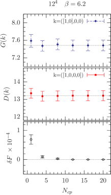
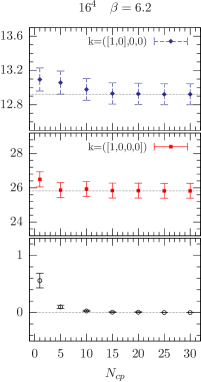
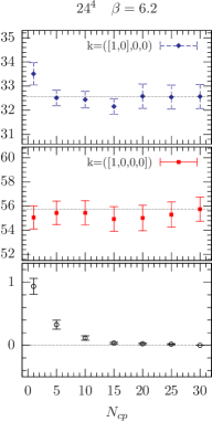
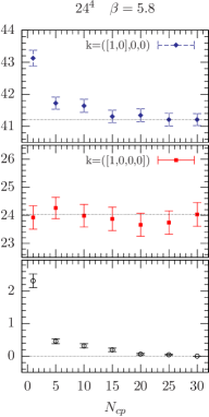
Figure 1: The upper panels show the ghost propagator $G(k)$ as average over two realizations $k=(1,0,0,0)$ and $k=(0,1,0,0)$ of the smallest lattice momentum, measured always on the best gauge copy among $N_{\rm cp}$ copies. In the middle panels the same dependence is shown for the gluon $D(k)$ propagator, however, as average over all four permutations of $k=(1,0,0,0)$. The lower panels show the relative difference $\delta F=1-F^{\texttt{cbc}}/F^{\texttt{bc}}$ of the corresponding current best functional values $F^{\texttt{cbc}}$ to the value $F^{\texttt{bc}}$ of the overall best copy.

III Results for the ghost and gluon propagators

III.1 Lattice samples

For the purpose of this study we have analyzed pure $SU(3)$ gauge configurations which have been thermalized with the standard Wilson action at three values of the inverse coupling constant $\beta=5.8$, $6.0$ and $6.2$. For thermalization an update cycle of one heatbath and four micro-canonical over-relaxation steps was used. As lattice sizes we used $16^{4}$, $24^{4}$ and $32^{4}$. For tests, exposing the inherent problems of the Gribov problem under the aspect of volume dependence, also smaller lattices ($8^{4}$ and $12^{4}$) have been considered at lower cost.

To each thermalized configuration $U$ a random set of $N_{\rm cp}{}$ local gauge transformation $\{g_{x}\}$ were assigned. Each of those served as starting point for a gauge fixing procedure for which we used standard over-relaxation with over-relaxation parameter tuned to $\omega=1.63$. Keeping all $U_{x,\mu}$ fixed this iterative procedure creates a sequence of local gauge transformations $g_{x}$ at sites $x$ with increasing values of the gauge functional (Eq. (5)). Thus, the final Landau gauge is iteratively approximated until the stopping criterion in terms of the transversality (see Eq. (6))

$$\max_{x}\left[\partial_{\mu}{}^{g}\!\!A_{\mu}(x)\right]^{2}<10^{-14}$$ (13)

is fulfilled. Consequently, each random start results in its own local maximum of the gauge functional. Certain extrema of the functional are found multiple times. In fact, this happened frequently on the small lattices, $8^{4}$ and $12^{4}$, but rather seldom on larger lattices. Note that we used the maximum in relation (13) which is very conservative. However, the precision of transversality dictates how symmetric the F-P operator $M$ can be considered. This is crucial for its inversion and thus dictates the final precision of the ghost propagator.

To study the dependence on Gribov copies of the propagators, in the course of $N_{\rm cp}{}$ repetitions for each $U$, the gauge copy with the largest functional value is stored under the name best copy (bc). The first gauge copy is also stored, labeled as first copy (fc). However, it is as good as any other arbitrarily selected gauge copy.

The more gauge copies one gets to inspect, the bigger the likeliness that the copy labeled as bc actually represents the absolute maximum of the functional in Eq. (5). With increasing number $N_{\rm cp}{}$ of copies the expectation value of gauge variant quantities, evaluated on bc representatives, is converging more or less rapidly as we will discuss next.

III.2 How severe is the lattice Gribov problem for the propagators?

First we present results of a combined study of the gluon and ghost propagators on the same sets of fc and bc representatives of our thermalized gauge field configurations. This allows us to assess the importance of the Gribov copy problem.

Numerically, it turns out that the dependence of the ghost propagator on the choice of the best copy is most severe for the smallest momentum. In addition, this depends on the lattice size and $\beta$. Therefore we studied first the dependence of the ghost and gluon propagators at lowest momentum on the (same) best copies as function of the number of gauge copies $N_{\rm cp}$ under inspection. This was done at $\beta=6.2$ where we used $12^{4}$, $16^{4}$ and $24^{4}$ lattices. The number of thermalized configurations used for these three lattice sizes are given in Table 1. To check the dependence on $\beta$ also a simulation at $\beta=5.8$ on a $24^{4}$ lattice was performed.

 

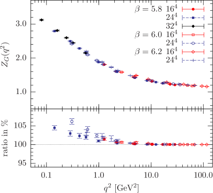
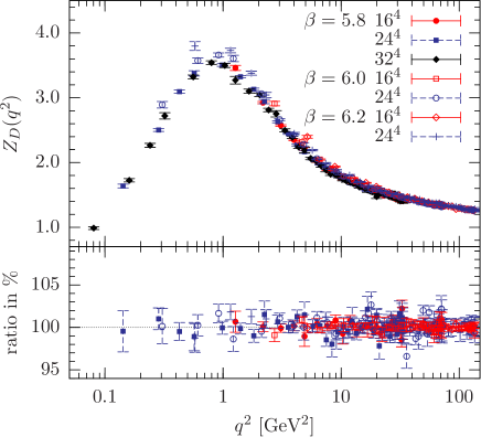
Figure 2: The upper panels show the dressing functions of the ghost $Z_{G}$ and gluon propagator $Z_{D}$ measured on best gauge copies as functions of the momentum $q^{2}$ (scaled to physical units at $\beta=5.8,6.0$ and $6.2$) using various lattice sizes. The lower panels show the ratio $\langle Z^{\rm fc}\rangle/\langle Z^{\rm bc}\rangle$ determined on first (fc) and best (bc) gauge copies using jackknife.

The results of this investigation are show in Fig. 1. While there the ghost propagator is shown as an average over the two realizations $k=(1,0,0,0)$ and $k=(0,1,0,0)$ of the smallest lattice momentum $q(k)$, the gluon propagator has been averaged over all four non-equivalent realizations. Note that $D(k)=D(-k)$. It is clearly visible that the expectation value of the gluon propagator does not change within errors as $N_{\rm cp}{}$ increases, independent of the lattice size and $\beta$. Contrarily, the ghost propagator at $\beta=5.8$ on a $24^{4}$ lattice saturates (on average) if calculated on the best among $N_{\rm cp}{}=15$ gauge copies. At $\beta=6.2$ the number of gauge fixings attempts reduces to $5\leq N_{\rm cp}{}\leq 10$ on a $16^{4}$ and $24^{4}$ lattice. On the $12^{4}$ lattice a small impact of Gribov copies is visible, namely $1<N_{\rm cp}{}\leq 5$. The lower panels of Fig. 1 show the relative difference $\delta F=1-F^{\texttt{cbc}}/F^{\texttt{bc}}$ of the corresponding (current best) functional values $F^{\texttt{cbc}}$ to the value $F^{\texttt{bc}}$ of the overall best copy after $N_{\rm cp}{}=20$, respectively $N_{\rm cp}{}=30$, attempts. This may serve as an indicator how large $N_{\rm cp}{}$ has to be on average for the chosen algorithm to have found a maximum of $F$ close to the global one.

In order to study further the low-momentum dependence of the gluon and ghost dressing functions, $Z_{D}$ and $Z_{G}$, as given by Eq. (1) and Eq. (2) we have performed similar simulations using lattice sizes $12^{4}$, $16^{4}$, $24^{4}$ and $32^{4}$ at $\beta=5.8$, 6.0 and 6.2. Following Ref. Necco and Sommer (2002) these values of $\beta$ correspond to $a^{-1}$=1.446 GeV, 2.118 GeV and 2.914 GeV using the Sommer scale $r_{0}=0.5$ fm. These values of the lattice spacing $a$ associated to $\beta$ turn out to be more appropriate as those formerly used by us and others (see Sternbeck et al. (2005a, b); Silva and Oliveira (2004); Leinweber et al. (1999)).

We have fixed a conservative number of $N_{\rm cp}{}=30$ gauge copies per thermalized configuration on a $16^{4}$ lattice and $N_{\rm cp}{}=40$ on a $24^{4}$ lattice. Both the gluon and the ghost propagator, respectively their dressing functions, have been measured on the same set of fc and bc copies. Due to the large amount of computing time necessary for the $32^{4}$ lattice we could afford to measure the ghost propagator for the first and best among only $N_{\rm cp}{}=10$ copies, which is certainly not enough.

The data for the gluon propagator $D(k)$ have been determined for all momenta at once. However, we used only a subset of momenta for the final analysis. In fact, inspired by Ref. Leinweber et al. (1999), only data $D(k)$ with $k$ lying in a cylinder with radius of one momentum unit along one of the diagonals $\hat{n}=1/2(\pm 1,\pm 1,\pm 1,\pm 1)$ have been selected. Since we are using a symmetric lattice structure only data with $k$ satisfying $\sum_{\mu}k^{2}_{\mu}-(\sum_{\mu}k_{\mu}\hat{n}_{\mu})^{2}\leq 1$ are surviving this cylindrical cut. In agreement with Leinweber et al. (1999) this recipe has drastically reduced lattice artifacts, in particular for large momenta. Additionally, we try to keep finite volume artifacts at lower momenta under control by removing all data $D(k)$ with one or more vanishing momentum components $k_{\mu}$ Leinweber et al. (1999). However, this we have done only for data on a $12^{4}$ and $16^{4}$ lattice. In Sec. III.3 we shall discuss in more detail finite volume effects at various momenta.

In view of this we have chosen appropriate sets of momenta for the ghost propagator, as listed in Table 1 in detail.

The final results of the dressing functions $Z_{D}$ and $Z_{G}$ measured on bc copies are shown in the upper panels of Fig. 2. All momenta $q(k)$ have been mapped to physical momenta using the lattice spacings $a$ given above. As expected the ghost dressing function diverges with decreasing momenta, while the gluon dressing function decreases after passing a turnover at about $q^{2}=0.8$ GeV². However, for the purpose of the expected infrared behavior given in Eq. (3) the data for momenta $q^{2}<0.25$ GeV² are not sufficiently abundant to extract a critical exponent $\kappa_{G}>0.5$ as expected from the Dyson-Schwinger approach. In particular, the fit parameters are not stable under a change of the upper momentum cutoff. The best fits give $\kappa_{G}\approx 0.25$.

In the lower panels of Fig. 2 we present the ratio of the dressing functions, $\langle Z^{\texttt{fc}}\rangle/\langle Z^{\texttt{bc}}\rangle$, calculated using jackknife from first and best gauge copies as a function of the momentum. There the data from simulations on a $32^{4}$ lattice have been excluded, since only $N_{\rm cp}{}=10$ gauge copies have been inspected which would result in an underestimate of the ratio $\langle Z^{\texttt{fc}}\rangle/\langle Z^{\texttt{bc}}\rangle$. As is clear from these panels we do not observe a systematic dependence on the choice of Gribov copies for the gluon propagator. In contrast the ghost propagator is systematically overestimated for fc (arbitrary) gauge copies. This effect holds up to momenta of about 2 GeV².

Comparing also the ratios for the ghost propagator at $q<1$ GeV, the rise at $\beta=6.0$ is obviously larger than that at $\beta=5.8$. In both cases the data are from simulations on a $24^{4}$ lattice. Thus, it seems that by increasing the physical volume (lower $\beta$) the effect of the Gribov ambiguity gets smaller if the same physical momentum is considered. This cannot be due to a too small number $N_{\rm cp}{}$ of inspected gauge copies since, judged from Fig. 1, $N_{\rm cp}{}=40$ seems to be on the safe side.

We conclude: the ghost propagator is systematically dependent on the choice of Gribov copies, while the impact on the gluon propagator is not resolvable within our statistics. However, there are indications that the dependence on Gribov copies decreases with increasing physical volume. This is also in agreement with the data listed in the two lattice studies Bakeev et al. (2004); Cucchieri (1997) of the $SU(2)$ ghost propagator $G$, while it is not explicitly stated there. In fact, in Ref. Bakeev et al. (2004) the ratio $G^{\texttt{fc}}/G^{\texttt{bc}}$ at $\beta=2.2$ on a $8^{4}$ lattice is larger than that on a $16^{4}$ lattice at the same physical momentum.

III.3 Systematic effects of lattice spacings and volumes

We remind that in Fig. 2 we have dropped all data related to a $16^{4}$ lattice with one or more vanishing momentum components $k_{\mu}$. According to Leinweber et al. (1999) this keeps finite volume effects for the gluon propagator under control. It is quite natural to analyze here the different systematic effects on the gluon and ghost propagators of changing either the lattice spacing $a$ or the physical volume $V$. However, due to the preselected set of momenta for the ghost propagator and the values chosen for $\beta$, we can study this here only in a limited way and in a region of intermediate momenta. For the gluon propagator this has been done in more detail by other authors (see e.g.  Bonnet et al. (2001)).

Keeping first the lattice spacing fixed we have found that both the ghost and gluon dressing functions calculated at the same physical momentum $q^{2}$ decrease as the lattice size $L^{4}$ is increased. This is illustrated for various momenta in Fig. 3. There both dressings functions versus the physical momentum are shown for different lattice sizes at either $\beta=5.8$ or $\beta=6.2$. Note, in this figure we have not dropped data with vanishing momentum components $k_{\mu}$ to emphasize the influence of a finite volume on those (low) momenta. We also show data from simulations on a $8^{4}$ and $12^{4}$ lattice. One clearly sees that the lower the momenta the larger the effect due to a finite volume. In comparison with $\beta=5.8$ this is even more drastic at $\beta=6.2$. At this $\beta$ the lattice spacing is about $a=0.068$ fm. Thus the largest volume considered at $\beta=6.2$ is about (1.6 fm)⁴, which is even smaller than the physical volume of a $16^{4}$ lattice at $\beta=5.8$.

Altogether we can state that for both dressing functions finite volume effects are clearly visible at volumes smaller than (2.2 fm)⁴, which corresponds to a $16^{4}$ lattice at $\beta=5.8$. The effect grows with decreasing momenta or decreasing lattice size (see the right panels in Fig. 3). At larger volumes, however, the data for $q>1$ GeV coincide within errors for the different lattice sizes (left panels). Even for $q<1$ GeV we cannot resolve finite volume effects for both dressing functions based on the data related to a $24^{4}$ and $32^{4}$ lattice.

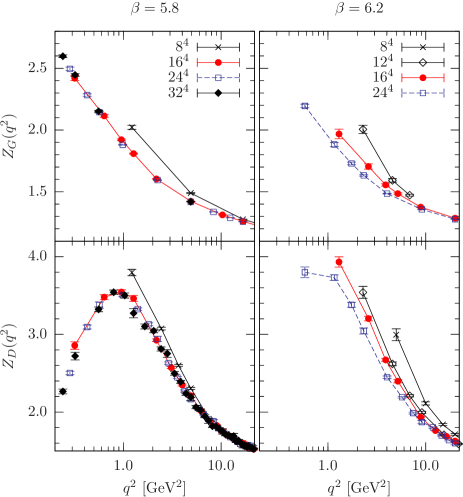
Figure 3: The ghost (upper panels) and gluon (lower panels) dressing functions are shown for different lattice sizes as functions of momentum $q^{2}$. The left panels show data at $\beta=5.8$ and the right ones at $\beta=6.2$. Only data on bc gauge copies are shown here. The lines are drawn to guide the eye.

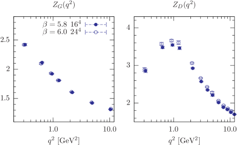
Figure 4: The ghost (left) and the gluon (right) dressing functions at (approximately) fixed physical volume $V_{1}\approx$(2.2 fm)⁴ are shown as functions of momentum $q^{2}$. The data at $\beta=5.8$ (6.0) correspond to a lattice spacing of about a=0.136 fm (0.093 fm). Only data on bc gauge copies are shown here.

 

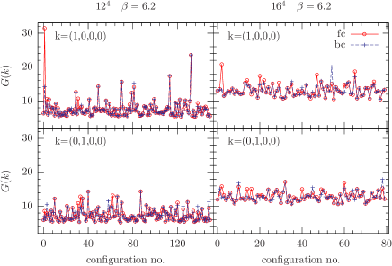
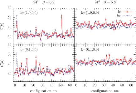
Figure 5: The time histories of the ghost propagator calculated on first (fc) and best (bc) gauge copies on a $12^{4}$, $16^{4}$ and $24^{4}$ lattice at $\beta=6.2$ and $24^{4}$ lattice at $\beta=5.8$. From left to right the corresponding runs listed in Table 1 are No.2, No.3, No.4/No.10 and No.1/No.8. The upper and lower panels show data for the lowest momentum realization $k=(1,0,0,0)$ and $k=(0,1,0,0)$, respectively.

Based on our chosen values for $\beta$ and the lattice sizes we can select equal physical volumes only approximately. Hence also the physical momenta are only approximately the same if the ghost and gluon dressing functions are compared at different $\beta$, e.g. at different lattice spacings. Therefore, it is difficult to analyze the systematic effect of changing $a$ if for both dressing functions small variations in $q^{2}$ are hidden. Consequently, in Fig. 4 we show the data for the ghost and gluon dressing functions approximately at the same physical volume $V\approx(2.2fm)^{4}$ for different $a$, albeit as functions of $q^{2}$. This allows us to disentangle by eyes a change of the data due to varying $a$ from the natural dependence of the propagators on $q^{2}$. Inspecting Fig. 4 one concludes that the gluon dressing function at the same physical momentum and volume increases with decreasing lattice spacing. A similar effect (beyond error bars) we cannot report for the ghost dressing function.

IV The problem of exceptional configurations

We turn now to a peculiarity of the ghost propagator at larger $\beta$ which has also been observed by some of us in an earlier $SU(2)$ study Bakeev et al. (2004). While inspecting our data we found, though rarely, that there are outliers in the Monte Carlo time histories of the ghost propagator at lowest momentum. Those outliers are not equally distributed around the average value, but are rather significantly larger than this.

In Fig. 5 we present time histories of the ghost propagator $G(k)$ measured of fc and bc gauge copies for two smallest momentum realizations $k=(1,0,0,0)$ and $k=(0,1,0,0)$, separately. From left to right the panels are ordered in increasing order of the lattice sizes $12^{4}$, $16^{4}$ and $24^{4}$ at $\beta=6.2$ and $24^{4}$ at $\beta=5.8$.

As can be seen from this figure in the majority extreme spikes are reduced (or even not seen) when the ghost propagator could be measured on a better gauge copy (bc) for a particular configuration. Furthermore, it is obvious that the exceptionality of a given gauge copy is exhibited not simultaneously for all different realizations of the lowest momentum. Consequently, to reduce the impact of such large values on the average ghost propagator one should better average over all momentum realizations giving rise to the same momentum $q$. This has been done for the results shown in Fig. 1 and 2 at least for the lowest momentum at $\beta=6.2$. However, compared to the gluon propagator it takes much more computing time to determine the ghost propagator for all its different realizations of momentum $q(k)$.

In addition, we have tried to find a correlation of such outliers in the history of the ghost propagator with other quantities measured in our simulations. For example we have checked whether there is a correlation between the values of the ghost propagator $G(k)$ as they appear in Fig. 5 with low-lying eigenvalues and eigenvectors of the F-P operator. They are apparent in the contribution of the lowest 10 F-P eigenmodes to the ghost propagator at this particular $k$. This we shall present in a subsequent publication Sternbeck et al. (2005c) where we shall discuss the spectral properties of the F-P operator and its relation to the ghost propagator.

V The running coupling

We shall now focus on the running coupling $\alpha_{s}(q^{2})$ as defined in Eq. (4) where $g^{2}_{0}/(4\pi)=3/(2\pi\beta)$ for $SU(3)$. Given the raw data for the gluon and ghost dressing functions on bc gauge copies the average $Z^{2}_{G}(q^{2})Z_{D}(q^{2})$ and its error have been estimated using the bootstrap method with drawing 500 random samples. Since the ghost-ghost-gluon-vertex renormalization function $Z_{1}$ has been set to one, there is an overall normalization factor which has been fixed by fitting the data for $q^{2}>q^{2}_{c}$ to the well-known perturbative results of the running coupling $\alpha_{\tt 2-loop}$ at 2-loop order (see also Bloch et al. (2004)). Defining $x\equiv q^{2}/\Lambda^{2}_{\tt 2-loop}$, the 2-loop running coupling is given by

$$\alpha_{\tt 2-loop}(x)=\frac{4\pi}{\beta_{0}\ln x}\left\{1-\frac{2\beta_{1}}{\beta^{2}_{0}}\frac{\ln(\ln x)}{\ln x}\right\}.$$ (14)

The $\beta$-function coefficients are $\beta_{0}=11$ and $\beta_{1}=51$ for the $SU(3)$ gauge group and are independent of the renormalization prescription. The value of $\Lambda_{\tt 2-loop}$ has been fixed by the same fit. The lower bound $q^{2}_{c}$ has been chosen such that an optimal value for $\chi^{2}/{\tt dof}$ has been achieved.

The results are shown in Fig. 6. There also the 1-loop contribution is shown where we used the same lower bound $q^{2}_{c}$. The best fit of the 2-loop expression to the data gives $\Lambda_{\tt 2-loop}$=0.88(7) GeV ($\chi^{2}/{\tt dof}=0.96$), while $\Lambda_{\tt 1-loop}$=0.64(7) is obtained ($\chi^{2}/{\tt dof}=1.05$) using just the 1-loop part. For $q^{2}_{c}$ we used $q^{2}_{c}=30$ GeV². The value for $\Lambda_{\tt 2-loop}$ is similar within errors to the $SU(2)$ result given in Ref. Bloch et al. (2004).

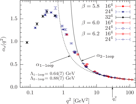
Figure 6: The running coupling $\alpha_{s}(q)$ as a function of momentum $q^{2}$ determined on bc gauge copies.

Approaching the infrared limit in Fig. 6 one clearly sees a running coupling $\alpha_{s}(q^{2})$ increasing for $q^{2}>0.4$ GeV². However, after passing a maximum at $q^{2}\approx 0.4$ GeV² $\alpha_{s}(q^{2})$ decreases again. Such turnover is in agreement with DSE results obtained on a torus Fischer et al. (2002); Fischer and Alkofer (2002); Fischer et al. (2005). Therefore, one can argue that this behavior is a finite lattice effect although we cannot resolve a difference between the different lattice sizes used. A similar infrared behavior for the running coupling has also been observed in different lattice studies Furui and Nakajima (2004b, a). But opposed to Furui and Nakajima (2004a) the existence of a turnover is independent on the choice of Gribov copy, since qualitatively, we have found the same behavior for $\alpha_{s}(q^{2})$ calculated on fc gauge copies.

For completeness we mention that running couplings decreasing in the infrared have also been found in lattice studies of the 3-gluon vertex Boucaud et al. (1998, 2003) and the quark-gluon vertex Skullerud and Kizilersu (2002).

Apart from the finite volume argument given above to explain such a behavior, which prevents us from seeing the limit $\alpha_{s}(0)\neq 0$ mentioned in the Introduction, one could also put into question whether one can really set $Z_{1}(q)=1$ at lower momenta. A recent investigation dedicated to the ghost-ghost-gluon-vertex renormalization function $Z_{1}(q)$ for the case of $SU(2)$ Cucchieri et al. (2004) supports that $Z_{1}(q)\approx 1$ at least for $q>1$ GeV.

VI Conclusions

We have reported on a numerical study of the gluon and ghost propagators in Landau gauge using several lattice sizes at $\beta=5.8$, $6.0$ and $6.2$. Studying the dependence on the choice of Gribov copies, it turns out that for the gluon propagator the effect of Gribov copies stays inside numerical uncertainty, while the impact on the ghost propagator increases as the momentum or $\beta$ is decreased. However, there are indications that the influence of Gribov copies decreases as the physical volume is increased. This is at least expected in the light of Ref. Zwanziger (2004). There it is argued that in the continuum expectation values of correlation functions $\langle A(x_{1})\ldots A(x_{n})\rangle$ over the fundamental modular region $\Lambda$ are equal to those over the Gribov region $\Omega$, since functional integrals are dominated by the common boundary of $\Lambda$ and $\Omega$. Thus Gribov copies inside $\Omega$ should not affect expectation values in the continuum.

While the effect of the Gribov ambiguity on the ghost propagator becomes smaller with increasing $\beta$, exceptionally large values appear in the history of the ghost propagator in agreement with what has been observed first in reference Bakeev et al. (2004). These outliers we have not seen simultaneously for all lattice momenta $k$ realizing the same lowest momentum $q(k)$. However, they are apparent in the contribution of the lowest 10 F-P eigenmodes to the ghost propagator at this particular $k$ Sternbeck et al. (2005c). Therefore it is good practice to measure the ghost propagator for more than one $k$ with the same momentum $q(k)$, in order to reduce the systematic errors coming from such exceptional values.

We have studied the effects of finite volume on the one hand and of finite lattice spacing on the other. The first ones are found to be essential for volumes smaller than $(2.2~{}\mathrm{fm})^{4}$ at the same $\beta$ whereas the discretization effects at the same volume are modest. Our available data did not allow us to extend this analysis to physical momenta below 1 GeV, where the Gribov ambiguity shows up and where a similar separation of finite volume and discretization effects would be desirable. However, we could observe from Fig. 2 that enlarging the volume by decreasing $\beta$ leads to a reduction of the systematic Gribov effect in the ghost propagator.

The dressing functions, $Z_{D}$ and $Z_{G}$, of the gluon and ghost propagators have allowed us to estimate the behavior of a running coupling $\alpha_{s}(q^{2})$ in a momentum subtraction scheme. Going from larger momenta $q^{2}$ to lower ones $\alpha_{s}(q^{2})$ is steadily increasing until $q^{2}\approx 0.4$ GeV². For $q^{2}<0.3$ GeV², however, $\alpha_{s}(q^{2})$ is decreasing. A decreasing running coupling at low momenta is in qualitative agreement with recent DSE results obtained on a torus Fischer et al. (2002); Fischer and Alkofer (2002); Fischer et al. (2005). Therefore one might conclude that the decrease is due to finite lattice volumes we used. It makes it questionable whether lattice simulations in near future can confirm the predicted infrared behavior of the gluon and ghost dressing functions with related exponents $\kappa_{D}=2\kappa_{G}$.

Appendix A Speeding up the inversion of the F-P operator

For the solution of the linear system $M\vec{\phi}=\vec{\psi}_{c}$ with symmetric matrix $M$, the conjugate gradient (CG) algorithm is the method of choice. Its convergence rate depends on the condition number, the ratio of largest to lowest eigenvalue of $M$. When all $U_{x,\mu}=\mathbb{1}$ obviously the F-P operator is minus the Laplacian $\Delta$ with a diagonal color substructure. Thus instead of solving $M\vec{\phi}=\vec{\psi}_{c}$ one rather solves the transformed system

$$[M\Delta^{-1}]\,(\Delta\vec{\phi}\,)=\vec{\psi}_{c}$$

In this way the condition number is reduced, however, the price to pay is one extra matrix multiplication by $\Delta^{-1}$ per iteration cycle. In terms of CPU time this should be more than compensated by the reduction of iterations.

The pre-conditioned CG algorithm (PCG) can be described as follows:

initialize:

$$\vec{r}^{\,(0)} = \vec{\psi}-M\vec{\phi}^{\,(0)},\quad\vec{p}^{\,(0)}=\Delta^{-1}\,\vec{r}^{\,(0)},$$

$$\gamma^{(0)} = (\vec{p}^{\,(0)},\vec{r}^{\,(0)})$$

start do loop: $$k=0,1,\ldots$$

$$\vec{z}^{\,(k)} = M\vec{p}^{\,(k)},\quad\alpha^{(k)}=\gamma^{\,(k)}/(\vec{z}^{\,(k)},\vec{p}^{\,(k)})$$

$$\vec{\phi}^{\,(k+1)} = \vec{\phi}^{\,(k)}+\alpha^{(k)}\vec{p}^{\,(k)}$$

$$\vec{r}^{\,(k+1)} = \vec{r}^{\,(k)}-\alpha^{(k)}\vec{z}^{\,(k)}$$

$$\vec{z}^{\,(k+1)} = \Delta^{-1}\,\vec{r}^{\,(k+1)}$$

$$\gamma^{(k+1)} = (\vec{z}^{\,(k+1)},\vec{r}^{\,(k+1)})$$

if $$(\gamma^{(k+1)}<\varepsilon)\quad\textit{exit do loop}$$

$$\vec{p}^{\,(k+1)} = \vec{z}^{\,(k+1)}+\frac{\gamma^{(k+1)}}{\gamma^{(k)}}\vec{p}^{\,(k)}$$

end do loop

Here $(\cdot,\cdot)$ denotes the scalar product.

To perform the additional matrix multiplication with $\Delta^{-1}$ we used two fast Fourier transformations $\mathcal{F}$, due to $(-\Delta)^{-1}=\mathcal{F}^{-1}\,q^{-2}(k)\,\mathcal{F}$. The performance we achieved is presented in Table 2. We conclude that on larger lattice sizes the reduction of iterations is about 70-75%, while the resulting reduction of CPU time depends on the lattice size. This is because we are using the fast Fourier transformations in a parallel CPU environment. If the ratio of used processors to the lattice size is small (see e.g. the data for $32^{4}$ lattice at this table), almost the same reductions of CPU time as for the number of iterations is achieved.

Further improvement may be achieved by using the multigrid Poisson solver to solve $\Delta\vec{z}^{\,(k)}=\vec{r}^{\,(k)}$. This method is supposed to perform better on parallel machines. Perhaps a further improvement is possible by using as pre-conditioning matrix $\widetilde{M}^{-1}=-\Delta^{-1}-\Delta^{-1}M_{1}\Delta^{-1}+\ldots$ which is an approximation of the F-P operator $M=-\Delta+M_{1}$ to a given order Zwanziger (1994) (see also Furui and Nakajima (2004b)). However, the larger the order, the more matrix multiplications per iteration cycle are required. This may reduce the overall performance. We have not checked so far which is the optimal order.

	CG		PCG		speed up
lattice	iter	CPU[sec]	iter	CPU[sec]	iter	CPU[sec]
$8^{4}$	1400	3.7	570	2.4	60%	35%
$16^{4}$	3900	240	1050	130	73%	46%
$32^{4}$	9900	13400	2250	3900	77%	71%

Table 2: The average number of iterations and CPU time per processor (PE) using the CG and PCG algorithm to invert the F-P operator are given. All inversions have been performed at $\beta=5.8$ with source $\delta^{bc}\exp(2\pi i\,k\!\cdot\!y)$ where $k=(1,0,0,0)$. To compare the different lattice sizes 4 PEs have always been used.

References

- Alkofer and von Smekal (2001) R. Alkofer and L. von Smekal, Phys. Rept. 353, 281 (2001), eprint hep-ph/0007355.
- Fischer and Alkofer (2003) C. S. Fischer and R. Alkofer, Phys. Rev. D67, 094020 (2003), eprint hep-ph/0301094.
- Lerche and von Smekal (2002) C. Lerche and L. von Smekal, Phys. Rev. D65, 125006 (2002), eprint hep-ph/0202194.
- Zwanziger (2002) D. Zwanziger, Phys. Rev. D65, 094039 (2002), eprint hep-th/0109224.
- Zwanziger (2004) D. Zwanziger, Phys. Rev. D69, 016002 (2004), eprint hep-ph/0303028.
- Zwanziger (1994) D. Zwanziger, Nucl. Phys. B412, 657 (1994).
- Gribov (1978) V. N. Gribov, Nucl. Phys. B139, 1 (1978).
- Kugo and Ojima (1979) T. Kugo and I. Ojima, Prog. Theor. Phys. Suppl. 66, 1 (1979).
- von Smekal et al. (1997) L. von Smekal, A. Hauck, and R. Alkofer, Phys. Rev. Lett. 79, 3591 (1997), eprint hep-ph/9705242.
- von Smekal et al. (1998) L. von Smekal, A. Hauck, and R. Alkofer, Ann. Phys. 267, 1 (1998), eprint hep-ph/9707327.
- Bloch et al. (2004) J. C. R. Bloch, A. Cucchieri, K. Langfeld, and T. Mendes, Nucl. Phys. B687, 76 (2004), eprint hep-lat/0312036.
- Taylor (1971) J. C. Taylor, Nucl. Phys. B33, 436 (1971).
- Cucchieri et al. (2004) A. Cucchieri, T. Mendes, and A. Mihara, JHEP 12, 012 (2004), eprint hep-lat/0408034.
- Langfeld et al. (2002) K. Langfeld, H. Reinhardt, and J. Gattnar, Nucl. Phys. B621, 131 (2002), eprint hep-ph/0107141.
- Gattnar et al. (2004) J. Gattnar, K. Langfeld, and H. Reinhardt, Phys. Rev. Lett. 93, 061601 (2004), eprint hep-lat/0403011.
- Bloch et al. (2003) J. C. R. Bloch, A. Cucchieri, K. Langfeld, and T. Mendes, Nucl. Phys. Proc. Suppl. 119, 736 (2003), eprint hep-lat/0209040.
- Oliveira and Silva (2005) O. Oliveira and P. J. Silva, AIP Conf. Proc. 756, 290 (2005), eprint hep-lat/0410048.
- Sternbeck et al. (2005a) A. Sternbeck, E.-M. Ilgenfritz, M. Müller-Preussker, and A. Schiller, Nucl. Phys. Proc. Suppl. 140, 653 (2005a), eprint hep-lat/0409125.
- Sternbeck et al. (2005b) A. Sternbeck, E.-M. Ilgenfritz, M. Müller-Preussker, and A. Schiller, AIP Conf. Proc. 756, 284 (2005b), eprint hep-lat/0412011.
- Furui and Nakajima (2004a) S. Furui and H. Nakajima, Phys. Rev. D70, 094504 (2004a), eprint hep-lat/0403021.
- Furui and Nakajima (2004b) S. Furui and H. Nakajima, Phys. Rev. D69, 074505 (2004b), eprint hep-lat/0305010.
- Fischer et al. (2005) C. S. Fischer, B. Grüter, and R. Alkofer (2005), eprint hep-ph/0506053.
- Fischer et al. (2002) C. S. Fischer, R. Alkofer, and H. Reinhardt, Phys. Rev. D65, 094008 (2002), eprint hep-ph/0202195.
- Fischer and Alkofer (2002) C. S. Fischer and R. Alkofer, Phys. Lett. B536, 177 (2002), eprint hep-ph/0202202.
- Cucchieri (1997) A. Cucchieri, Nucl. Phys. B508, 353 (1997), eprint hep-lat/9705005.
- Bakeev et al. (2004) T. D. Bakeev, E.-M. Ilgenfritz, M. Müller-Preussker, and V. K. Mitrjushkin, Phys. Rev. D69, 074507 (2004), eprint hep-lat/0311041.
- Nakajima and Furui (2004) H. Nakajima and S. Furui, Nucl. Phys. Proc. Suppl. 129, 730 (2004), eprint hep-lat/0309165.
- Silva and Oliveira (2004) P. J. Silva and O. Oliveira, Nucl. Phys. B690, 177 (2004), eprint hep-lat/0403026.
- Leinweber et al. (1999) D. B. Leinweber, J. I. Skullerud, A. G. Williams, and C. Parrinello, (UKQCD), Phys. Rev. D60, 094507 (1999), eprint hep-lat/9811027.
- Suman and Schilling (1996) H. Suman and K. Schilling, Phys. Lett. B373, 314 (1996), eprint hep-lat/9512003.
- Necco and Sommer (2002) S. Necco and R. Sommer, Nucl. Phys. B622, 328 (2002), eprint hep-lat/0108008.
- Bonnet et al. (2001) F. D. R. Bonnet, P. O. Bowman, D. B. Leinweber, A. G. Williams, and J. M. Zanotti, Phys. Rev. D64, 034501 (2001), eprint hep-lat/0101013.
- Sternbeck et al. (2005c) A. Sternbeck, E.-M. Ilgenfritz, M. Müller-Preussker, and A. Schiller, in progress (2005c).
- Boucaud et al. (1998) P. Boucaud, J. P. Leroy, J. Micheli, O. Pene, and C. Roiesnel, JHEP 10, 017 (1998), eprint hep-ph/9810322.
- Boucaud et al. (2003) P. Boucaud et al., JHEP 04, 005 (2003), eprint hep-ph/0212192.
- Skullerud and Kizilersu (2002) J. Skullerud and A. Kizilersu, JHEP 09, 013 (2002), eprint hep-ph/0205318.