DESY 05-070

CERN-PH-TH/2005-45

FTUAM-05-2

IFT-UAM-CSIC/05-16

May 2005

A perturbative study of two four-quark operators
in finite volume renormalization schemes

Starting from the QCD Schrödinger functional (SF), we define a family of renormalization schemes for two four-quark operators, which are, in the chiral limit, protected against mixing with other operators. With the appropriate flavour assignments these operators can be interpreted as part of either the $\Delta F=1$ or $\Delta F=2$ effective weak Hamiltonians. In view of lattice QCD with Wilson-type quarks, we focus on the parity odd components of the operators, since these are multiplicatively renormalized both on the lattice and in continuum schemes. We consider 9 different SF schemes and relate them to commonly used continuum schemes at one-loop order of perturbation theory. In this way the two-loop anomalous dimensions in the SF schemes can be inferred. As a by-product of our calculation we also obtain the one-loop cutoff effects in the step-scaling functions of the respective renormalization constants, for both O($a$) improved and unimproved Wilson quarks. Our results will be needed in a separate study of the non-perturbative scale evolution of these operators.

1 Introduction

In the Standard Model, four-quark operators typically arise as effective interaction vertices when integrating out the large scale physics associated with the weak interactions. Examples are the $\Delta B=2$ operators

$$O^{\Delta B=2}=\left(\bar{b}\gamma_{\mu}(1-\gamma_{5})d\right)^{2},$$ (1.1)

which mediate $B^{0}$–$\bar{B}^{0}$ mixing or their analogues in the case of kaons. Hence, the quantities of interest are matrix elements of four-quark operators between hadronic states, which are inherently non-perturbative in nature. On the other hand, the four-quark operators are originally obtained in perturbation theory and renormalized at a large scale, using e.g. the minimal scheme (MS) of dimensional regularization. If lattice QCD is used for the calculation of the hadronic matrix elements, the matching to the perturbative renormalization schemes poses a problem, since the scale differences involved are potentially large. A general strategy to solve this problem has been proposed some time ago [?]: its starting point is the definition of an intermediate scheme, where the finite space-time volume is used to set the renormalization scale. Finite-size-scaling techniques then allow to step up the energy scale recursively until the perturbative regime is reached, where the continuum schemes can be safely matched in perturbation theory. Previous applications include the running coupling [?] and quark mass [?,?,?], moments of structure functions [?–?], and the static-light axial current [?,?].

This paper is part of a project to apply this strategy to two particularly important four-quark operators with phenomenological applications to $B^{0}$–$\bar{B}^{0}$ or $K^{0}$–$\bar{K}^{0}$ mixing and non-leptonic kaon decays [?–?]. We use the QCD Schrödinger functional to define a family of finite volume renormalization schemes, and report our results for the perturbative matching to more commonly used renormalization schemes. The matching procedure is done in two steps: first the Schrödinger functional is regularized on the lattice with Wilson-type quarks, and the renormalized operators are related to the standard lattice scheme, defined by minimal subtraction of logarithms. Then, using results from the literature, this lattice scheme can be related to a continuum scheme, such as dimensional reduction (DRED) or one of the minimal subtraction schemes ($\rm MS$) in dimensional regularization. Since the two-loop anomalous dimensions are known in these schemes, the one-loop matching then allows the two-loop anomalous dimensions to be inferred in the SF schemes, too.

The paper is organized as follows: in section 2 we start with the definition of the operators and their correlation functions in the Schrödinger functional, which are then used to formulate the renormalization conditions. After a short review of perturbative matching equations between different renormalization schemes (section 3), we collect the equations for the reference schemes (section 4) and report the results of our one-loop computation (section 5). In view of the corresponding non-perturbative computation with Wilson-type quarks, we then discuss perturbative lattice artefacts in the step-scaling functions (section 6) and present our conclusions.

2 Definitions and setup

The four-quark operators we would like to renormalize are of the form

$$O^{\pm}_{\rm LL}=\frac{1}{2}\left[(\bar{\psi}_{1}\gamma_{\mu}(1-\gamma_{5})\psi_{2})(\bar{\psi}_{3}\gamma_{\mu}(1-\gamma_{5})\psi_{4})\pm(\bar{\psi}_{1}\gamma_{\mu}(1-\gamma_{5})\psi_{4})(\bar{\psi}_{3}\gamma_{\mu}(1-\gamma_{5})\psi_{2})\right],$$ (2.2)

where the subscript ${\rm LL}$ refers to the Dirac structure of two left-handed currents, and it is understood that colour indices are contracted within the quark bilinears in round brackets. In order to make contact with phenomenological applications, one just needs to assign the physical quark flavours. For instance, with the identifications

$$\psi_{1}=\psi_{3}=s,\qquad\psi_{2}=\psi_{4}=d,$$ (2.3)

the operator $O^{-}_{\rm LL}$ vanishes while the matrix elements of $O^{+}_{\rm LL}$ appear in the $K^{0}$–$\bar{K}^{0}$ mixing amplitude. Replacing strange by bottom quarks, the same operator mediates $B^{0}$–$\bar{B}^{0}$ mixing. If instead one identifies

$$\psi_{1}=s,\qquad\psi_{2}=d,\qquad\psi_{3}=\psi_{4}=u,c,$$ (2.4)

one obtains the $\Delta S=1$ operators relevant to the $\Delta I=1/2$ rule in non-leptonic kaon decays, in a framework where the charm quark remains an active degree of freedom.

The operators (2.2) can be decomposed in parity-even and -odd components:

$$O^{\pm}_{\rm LL}\equiv O^{\pm}_{\rm(V-A)(V-A)}=O^{\pm}_{\rm VV+AA}-O^{\pm}_{\rm VA+AV},$$ (2.5)

where $\rm V,A$ refer to the Dirac structure of vector and axial vector currents, respectively. In the following we will work with the parity-odd component of the operators,

$$O^{\pm}_{\rm VA+AV}=\frac{1}{2}\left[(\bar{\psi}_{1}\gamma_{\mu}\psi_{2})(\bar{\psi}_{3}\gamma_{\mu}\gamma_{5}\psi_{4})+(\bar{\psi}_{1}\gamma_{\mu}\gamma_{5}\psi_{2})(\bar{\psi}_{3}\gamma_{\mu}\psi_{4})\pm(\psi_{2}\leftrightarrow\psi_{4})\right],$$ (2.6)

rather than staying with the product of two left-handed currents (2.2) as induced by the Standard Model weak interactions. Note that in regularizations that preserve chiral symmetry, parity-even and parity-odd components are related by chiral symmetry and are thus renormalized in the same way. However, the situation changes in lattice regularizations with Wilson-type quarks: while the parity-odd operators $O^{\pm}_{\rm VA+AV}$ are multiplicatively renormalizable [?], their parity-even partners $O^{\pm}_{\rm VV+AA}$ share the lattice symmetries with four other four-quark operators, which leads to a complicated operator mixing problem. Although this problem can be solved non-perturbatively [?], it is a source of additional uncertainties and systematic errors. In this paper this problem is circumvented by imposing renormalization conditions on the parity-odd operator components. Besides its technical advantage this strategy makes sense also from a practical point of view: as has been demonstrated in [?], the introduction of non-standard chirally twisted mass terms (“twisted mass QCD”) redefines the physical parity symmetry so that the parity-odd operator components can play the rôle of operators with either physical parity. As a result, the hadronic matrix elements of operators with even physical parity can be obtained from correlation functions which only involve the lattice operators (2.6). We conclude that our choice to renormalize these parity-odd operator components is irrelevant for chirally symmetric regularizations, but it is advantageous with Wilson-type quarks and does not imply any prejudice on possible phenomenological applications.

2.1 Renormalization conditions

We now choose the lattice regularization with Wilson quarks, possibly O($a$) improved by the Sheikholeslami–Wohlert term in the action [?]. For unexplained notation we refer the reader to ref. [?]. We assume that the bare operators (2.6) are defined locally on the lattice, i.e. all quark and antiquark fields are taken at the same space-time point. To formulate renormalization conditions for the renormalized operators

$$(O_{\rm R})^{\pm}_{\rm VA+AV}=Z^{\pm}_{\rm VA+AV}O^{\pm}_{\rm VA+AV},$$ (2.7)

we use the standard set-up of the Schrödinger functional [?,?] as described in [?]. We consider generic source fields made up of boundary quarks and antiquarks,

$${\cal O}_{12}[\Gamma] = a^{6}\sum_{\rm y,z}\bar{\zeta}_{1}({\bf y})\Gamma\zeta_{2}({{\bf z}}),$$ (2.8)

$${\cal O}^{\prime}_{12}[\Gamma] = a^{6}\sum_{\rm y,z}\bar{\zeta}\kern 1.0pt^{\prime}_{1}({\bf y})\Gamma\zeta\kern 1.0pt^{\prime}_{2}({{\bf z}}),$$ (2.9)

where $\Gamma$ is a Dirac matrix that must anticommute with $\gamma_{0}$ as otherwise the source field vanishes. This is due to the projectors $P_{\pm}=\frac{1}{2}(1\pm\gamma_{0})$, which are implicit in the boundary quark and antiquark fields,

$$\zeta({\bf x})=P_{-}\zeta({\bf x}),\qquad\bar{\zeta}({\bf x})=\bar{\zeta}({\bf x})P_{+},$$ (2.10)

and similarly for the primed fields. The presence of the projectors limits the possible Dirac structures for the quark bilinears at the time boundaries. For instance, it is not possible to define scalar quark bilinear sources, unless one introduces a non-vanishing angular momentum. However, finite momenta typically increase the lattice artefacts, and lead to poor signal-to-noise ratios in numerical simulations, so that we are not going to pursue this further.

The renormalization conditions will be imposed in the massless theory, so that the renormalization constants and the renormalized coupling are quark mass independent by construction. In the absence of chirally twisted mass terms, standard parity is an exact symmetry of the lattice-regularized Schrödinger functional. In order to renormalize the parity-odd operators (2.6) we thus need a total source with negative parity which contains at least 2 quark bilinear sources. Because of the above mentioned problem with the projectors at the time boundaries, we decided to introduce a fifth “spectator quark” and use correlation functions of the generic form:

$$F^{\pm}[\Gamma_{A},\Gamma_{B},\Gamma_{C}](x_{0})=L^{-3}\left\langle{\cal O}_{21}[\Gamma_{A}]O^{\pm}_{\rm VA+AV}(x){\cal O}_{45}[\Gamma_{B}]{\cal O}^{\prime}_{53}[\Gamma_{C}]\right\rangle.$$ (2.11)

The corresponding Feynman diagram is given in the left of fig. 1, where the quark lines correspond to the boundary-to-volume quark propagators $H(x),H^{\prime}(x)$ of refs. [?,?], and to the boundary-to-boundary propagator $K$ of ref. [?], which contains an explicit time-like link variable from Euclidean time $T-a$ to $T$.

We then consider the 5 specific cases

$$F^{\pm}_{1}(x_{0}) = F^{\pm}[\gamma_{5},\gamma_{5},\gamma_{5}](x_{0}),$$ (2.12)

$$F^{\pm}_{2}(x_{0}) = \frac{1}{6}\sum_{i,j,k=1}^{3}\varepsilon_{ijk}F^{\pm}[\gamma_{i},\gamma_{j},\gamma_{k}](x_{0}),$$ (2.13)

$$F^{\pm}_{3}(x_{0}) = \frac{1}{3}\sum_{k=1}^{3}F^{\pm}[\gamma_{5},\gamma_{k},\gamma_{k}](x_{0}),$$ (2.14)

$$F^{\pm}_{4}(x_{0}) = \frac{1}{3}\sum_{k=1}^{3}F^{\pm}[\gamma_{k},\gamma_{5},\gamma_{k}](x_{0}),$$ (2.15)

$$F^{\pm}_{5}(x_{0}) = \frac{1}{3}\sum_{k=1}^{3}F^{\pm}[\gamma_{k},\gamma_{k},\gamma_{5}](x_{0}).$$ (2.16)

These correlation functions describe transitions between parity-even and -odd states at the Euclidean time boundaries, mediated by the parity-odd four-quark operators. In particular, parity-even scalar or axial vector states are produced at the lower time boundary by taking appropriate combinations of pseudoscalar and vector states.

In order to obtain renormalization conditions for the four-quark operators based on these correlation functions, we first have to take care of the source field renormalization. As the boundary quark and antiquark fields are all renormalized multiplicatively by the same renormalization constant [?], this can easily be achieved by forming appropriate ratios of correlation functions. More precisely, with the boundary-to-boundary correlators

$$f_{1} = -\dfrac{1}{2L^{6}}\left\langle{\cal O}_{12}[\gamma_{5}]{\cal O}^{\prime}_{21}[\gamma_{5}]\right\rangle,$$ (2.17)

$$k_{1} = -\dfrac{1}{6L^{6}}\sum_{k=1}^{3}\left\langle{\cal O}_{12}[\gamma_{k}]{\cal O}^{\prime}_{21}[\gamma_{k}]\right\rangle,$$ (2.18)

we consider the following 9 ratios of correlation functions

$$h^{\pm}_{i}(x_{0}) = \dfrac{F^{\pm}_{i}(x_{0})}{f_{1}^{3/2}},\quad i={1,\ldots,5}$$ (2.19)

$$h^{\pm}_{6}(x_{0}) = \dfrac{F^{\pm}_{2}(x_{0})}{k_{1}^{3/2}},$$ (2.20)

$$h^{\pm}_{i+4}(x_{0}) = \dfrac{F^{\pm}_{i}(x_{0})}{f_{1}^{1/2}k_{1}},\quad i={3,4,5}.$$ (2.21)

In these ratios the renormalization of the boundary fields cancels out, i.e. the renormalized ratios are obtained by multiplying with the appropriate four-quark operator renormalization constant. A renormalization condition is now obtained by choosing one of the ratios (2.21), setting the renormalized quark mass to zero, and specifying $T/L$, $x_{0}/L$ and the angle $\theta$ of the spatial boundary conditions [?].

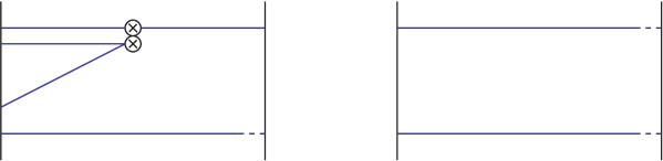
Figure 1: The Feynman diagrams for the four-quark correlation functions $F^{\pm}_{s}(x_{0})$ and the boundary-to-boundary correlators $f_{1},k_{1}$ at tree level. Euclidean time goes from left to right. The double blob indicates the four-quark operator insertion and the dashed links indicate the explicit time-like link variable in the boundary-to-boundary quark propagators.

All parameters are then fixed, and $L$ remains the only scale in the system. Then one requires

$$Z^{\pm}_{\rm VA+AV;s}(g_{0},a\mu)h_{s}^{\pm}(x_{0})=h_{s}^{\pm}(x_{0})|_{g_{0}=0},$$ (2.22)

where the RHS is the free field theory result. The renormalization constant $Z^{\pm}_{\rm VA+AV;s}$ is thus obtained at the renormalization scale $\mu=1/L$, and depends implicitly on all the parameter choices made. In practice, we followed refs. [?,?] and always set $T=L$, $x_{0}=L/2$ and $\theta=0.5$. This leaves us with 9 different SF schemes labelled by $s=1,\ldots,9$ in eq. (2.22). While there are good arguments for choosing $T=L$ [?], there are in general no a priori criteria for a good parameter choice. This can only be judged a posteriori by comparing non-perturbative and perturbative data, or by looking at the apparent convergence of the perturbative expansion of the anomalous dimensions. As it will turn out, there is considerable variation among our 9 choices of renormalization schemes.

3 Anomalous operator dimensions in perturbation theory

Operators and parameters are renormalized at the renormalization scale $\mu$, which in the SF schemes is identified with $1/L$. A change of scale is then governed by the renormalization group. Let us consider QCD with $N_{\rm f}$ mass degenerate quark flavours and $N$ colours, and its Euclidean correlation functions of gauge-invariant composite operators. Limiting ourselves to multiplicatively renormalizable operators, any renormalized $n$-point functions of such operators,

$$G_{n}(x_{1},\ldots,x_{n})=\left\langle O_{1}(x_{1})\cdots O_{n}(x_{n})\right\rangle,$$ (3.23)

satisfies the Callan–Symanzik equation

$$\left\{\mu\dfrac{\partial}{\partial\mu}+\beta(g)\dfrac{\partial}{\partial g}+\tau(g)m\dfrac{\partial}{\partial m}-\sum_{i=1}^{n}\gamma_{O_{i}}(g)\right\}G_{n}=0.$$ (3.24)

The renormalization group functions $\beta$, $\tau$ and $\gamma$ are the $\beta$-function for the coupling and the anomalous dimensions for the quark mass and composite operators respectively. In quark mass independent schemes the renormalization group functions only depend on the renormalized coupling and have perturbative expansions of the form

$$\beta(g) \buildrel{g}\rightarrow 0\over{\sim} -g^{3}\sum_{k=0}^{\infty}b_{k}g^{2k},$$ (3.25)

$$\tau(g) \buildrel{g}\rightarrow 0\over{\sim} -g^{2}\sum_{k=0}^{\infty}d_{k}g^{2k},$$ (3.26)

$$\gamma(g) \buildrel{g}\rightarrow 0\over{\sim} -g^{2}\sum_{k=0}^{\infty}\gamma_{k}g^{2k}.$$ (3.27)

The coefficients are scheme-dependent in general, except for $b_{0},b_{1}$ and $d_{0},\gamma_{0}$. In the normalization adopted here we have (see refs. [?,?,?] for the coefficients up to $k=3$ in the ${\rm\overline{MS\kern-0.50003pt}\kern 0.50003pt}$ scheme and for further references):

$$b_{0} = \left\{\frac{11}{3}N-\frac{2}{3}N_{\rm f}\right\}(4\pi)^{-2},$$ (3.28)

$$d_{0} = \dfrac{3(N^{2}-1)}{N}(4\pi)^{-2},$$ (3.29)

$$b_{1} = \left\{\frac{34}{3}N^{2}-\left(\frac{13}{3}N-N^{-1}\right)N_{\rm f}\right\}(4\pi)^{-4}.$$ (3.30)

Denoting the anomalous dimensions for the operators $O_{\rm VA+AV}^{\pm}$ by $\gamma^{\pm}$, their leading order coefficients are given by [?,?]

$$\gamma_{0}^{\pm}=\dfrac{\pm 6(N\mp 1)}{N}(4\pi)^{-2}.$$ (3.31)

The universality of these coefficients can easily be understood by changing to another quark mass independent scheme. This amounts to finite renormalizations of the form

$$g^{\prime} = g\sqrt{{\cal X}_{\rm g}(g)},$$ (3.32)

$$m^{\prime} = m{\cal X}_{\rm m}(g),$$ (3.33)

$$O^{\prime}_{\rm R} = O_{\rm R}{\cal X}_{O}(g).$$ (3.34)

The $n$-point functions of the primed operators satisfy again a Callan–Symanzik equation of the form (3.24), and the respective renormalization group functions are then related as follows

$$\beta^{\prime}(g^{\prime}) = \left\{\beta(g)\dfrac{\partial g^{\prime}}{\partial g}\right\}_{g=g(g^{\prime})},$$ (3.35)

$$\tau^{\prime}(g^{\prime}) = \left\{\tau(g)+\beta(g)\dfrac{\partial}{\partial g}\ln{\cal X}_{\rm m}(g)\right\}_{g=g(g^{\prime})},$$ (3.36)

$$\gamma^{\prime}(g^{\prime}) = \left\{\gamma(g)+\beta(g)\dfrac{\partial}{\partial g}\ln{\cal X}_{O}(g)\right\}_{g=g(g^{\prime})}.$$ (3.37)

Expanding the renormalization factors in perturbation theory,

$${\cal X}(g)\buildrel{g}\rightarrow 0\over{\sim}1+\sum_{k=1}^{\infty}{\cal X}^{(k)}g^{2k}.$$ (3.38)

one finds that $b_{0},b_{1}$, and $d_{0},\gamma_{0}$ remain indeed unchanged, and for the next-to-leading order anomalous dimensions one arrives at

$$d_{1}^{\prime} = d_{1}+2b_{0}{\cal X}_{\rm m}^{(1)}-d_{0}{\cal X}_{\rm g}^{(1)},$$ (3.39)

$$\gamma_{1}^{\prime} = \gamma_{1}+2b_{0}{\cal X}_{O}^{(1)}-\gamma_{0}{\cal X}_{\rm g}^{(1)}.$$ (3.40)

Hence, if $\gamma_{1}$ is known from a two-loop calculation in some reference scheme, it can be obtained in any other scheme by relating the schemes at one-loop order, thereby avoiding a direct two-loop computation. The situation for any multiplicatively renormalizable operator hence is the same as with the quark mass, where the two-loop anomalous dimension in the SF scheme has been obtained along these lines [?].

4 Reference schemes

The two-loop anomalous dimensions $\gamma_{1}^{\pm}$ have been computed for a variety of schemes [?–?]. The first computation was performed by Altarelli and collaborators [?], using dimensional reduction (DRED) [?]. This result was later confirmed by Buras and Weisz [?], who used dimensional regularization with both the naive and the ’t Hooft–Veltman definition of $\gamma_{5}$ in $D$ dimensions [?]. In the DRED scheme, but with the renormalized coupling defined in the ${\rm\overline{MS\kern-0.50003pt}\kern 0.50003pt}$ scheme (this differs from the renormalized coupling used in [?]), the two-loop anomalous dimension takes the form

$$\gamma^{\pm}_{1,\rm DRED}=\dfrac{N\mp 1}{2N}\left\{\frac{22}{3}N^{2}-21-\frac{4}{3}NN_{\rm f}\pm\left(\frac{113}{3}N+\frac{57}{N}-\frac{20}{3}N_{\rm f}\right)\right\}(4\pi)^{-4}.$$ (4.41)

For later reference we also quote the corresponding results in the NDR (“dimensional regularization with naive $\gamma_{5}$”) and HVDR (“dimensional regularization with ’t Hooft–Veltman $\gamma_{5}$”) schemes, as defined in [?]

$$\gamma^{\pm}_{1,\rm NDR} = \dfrac{N\mp 1}{2N}\left\{-21\pm\left(\frac{57}{N}-\frac{19}{3}N+\frac{4}{3}N_{\rm f}\right)\right\}(4\pi)^{-4},$$ (4.42)

$$\gamma^{\pm}_{1,\rm HVDR} = \dfrac{N\mp 1}{2N}\left\{\frac{88}{3}N^{2}-21-\frac{16}{3}NN_{\rm f}\pm\left(\frac{157}{3}N+\frac{57}{N}-\frac{28}{3}N_{\rm f}\right)\right\}(4\pi)^{-4}.$$ (4.43)

In order to obtain the two-loop anomalous dimensions in the SF schemes, we need the one-loop relations between the renormalized operators and coupling constants,

$$\left(O^{\pm}_{\rm VA+AV}\right)_{\rm SF} = \left(O^{\pm}_{\rm VA+AV}\right)_{\rm DRED}{\cal X}_{\rm SF,DRED}^{\pm}(\bar{g}),$$ (4.44)

$$\bar{g}_{\rm SF}^{2}(L) = \bar{g}^{2}(\mu){\cal X}_{g}(\bar{g}).$$ (4.45)

Here we have denoted the ${\rm\overline{MS\kern-0.50003pt}\kern 0.50003pt}$ coupling by $\bar{g}$, and we assume that the SF coupling has been defined for $N=3$ colours as in [?,?]. There, also the one-loop coefficient for the matching of the couplings has been determined:

$${\cal X}_{g}^{(1)} = 2b_{0}\ln(\mu L)-\dfrac{1}{4\pi}\left(c_{1,0}+c_{1,1}N_{\rm f}\right),$$ (4.46)

$$c_{1,0} = 1.25563(4),$$ (4.47)

$$c_{1,1} = 0.039863(2).$$ (4.48)

The one-loop relation between the renormalized operators will be established in two steps, by first converting to a lattice renormalization scheme ($\rm lat$), which is obtained by minimally subtracting the logarithms [?]. This yields the one-loop relation

$$\left(O_{\rm VA+AV}^{\pm}\right)_{\rm SF}=\left(O_{\rm VA+AV}^{\pm}\right)_{\rm lat}{\cal X}_{\rm SF,lat}^{\pm}(g_{\rm lat}),$$ (4.49)

which will be discussed in more detail in the next section. On the other hand, the relation between the operators in the ${\rm lat}$-scheme and DRED has been established in refs. [?,?,?]. Defining the finite renormalization factor through

$$(O_{\rm VA+AV}^{\pm})_{\rm DRED}=(O_{\rm VA+AV}^{\pm})_{\rm lat}{\cal X}_{\rm DRED,lat}^{\pm}(g_{\rm lat}),$$ (4.50)

the one-loop coefficient is given by

$${\cal X}_{\rm DRED,lat}^{\pm(1)}=\left\{Nz_{1}\pm z_{0}+N^{-1}z_{-1}\right\}(4\pi)^{-2},$$ (4.51)

with coefficients

$$z_{1} = \frac{1}{2}\left(\Delta_{\gamma_{\mu}}+\Delta_{\gamma_{\mu}\gamma_{5}}+2\Delta_{\Sigma_{1}}+1\right),$$ (4.52)

$$z_{0} = \frac{1}{2}\left(\Delta_{\gamma_{\mu}}+\Delta_{\gamma_{\mu}\gamma_{5}}-\Delta_{1}-\Delta_{\gamma_{5}}-1\right),$$ (4.53)

$$z_{-1} = \frac{1}{2}\left(\Delta_{1}+\Delta_{\gamma_{5}}\right)-\left(\Delta_{\gamma_{\mu}}+\Delta_{\gamma_{\mu}\gamma_{5}}+\Delta_{\Sigma_{1}}\right).$$ (4.54)

The $\Delta$’s have been defined in [?,?] and are related to the quark propagator and vertex functions of quark bilinears. Though gauge parameter dependent in general, the above linear combinations are gauge-independent, and a numerical evaluation yields [?,?,?],

$$[z_{1},z_{0},z_{-1}]=\begin{cases}\left[-14.06090(9),\hphantom{+}5.7854(1),\hphantom{0}8.2755(2)\right]&\text{for $c_{\rm sw}=1$},\\ \left[-17.70704(7),-0.9331(1),18.6402(2)\right]&\text{for $c_{\rm sw}=0$},\end{cases}$$ (4.55)

where to this order of perturbation theory $c_{\rm sw}\equiv c_{\rm sw}^{(0)}=0,1$ refers to standard and O($a$) improved Wilson quarks, respectively. With $N=3$, we obtain

$${\cal X}_{\rm DRED,lat}^{+(1)} = \begin{cases}-0.213020(2)&\text{for $c_{\rm sw}=1$},\\ -0.302956(2)&\text{for $c_{\rm sw}=0$},\end{cases}$$ (4.56)

$${\cal X}_{\rm DRED,lat}^{-(1)} = \begin{cases}-0.286293(2)&\text{for $c_{\rm sw}=1$},\\ -0.291138(2)&\text{for $c_{\rm sw}=0$}.\end{cases}$$ (4.57)

Finally, the desired one-loop relation between the SF schemes and the DRED scheme is obtained by combining eqs. (4.49),(4.50), which to one-loop order implies

$${\cal X}_{\rm SF,DRED}^{\pm(1)}={\cal X}_{\rm SF,lat}^{\pm(1)}-{\cal X}_{\rm DRED,lat}^{\pm(1)}.$$ (4.58)

The two-loop anomalous dimensions are then related by formula (3.40), identifying the SF and DRED schemes with the primed and unprimed schemes, respectively.

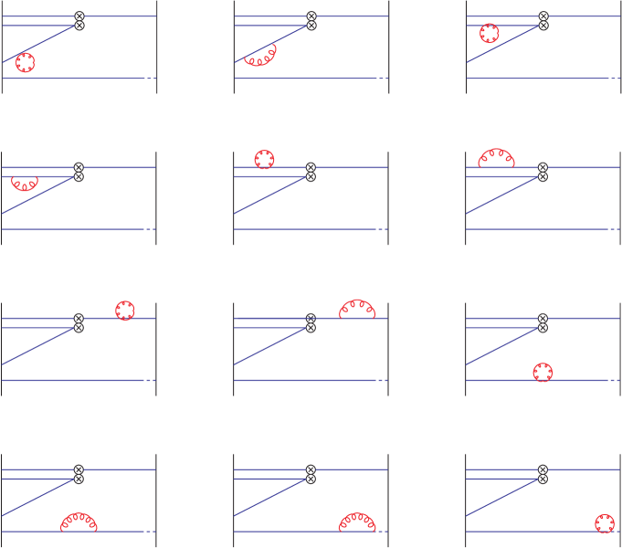
Figure 2: Feynman diagrams of the self-energy type.

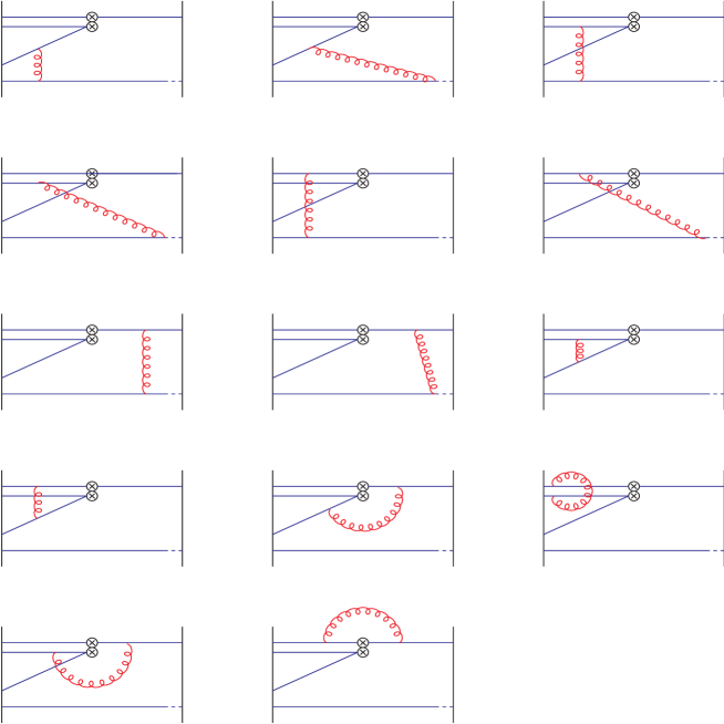
Figure 3: The remaining Feynman diagrams at one-loop order, which are not of the self-energy type.

5 One-loop results

The perturbative expansion of the finite volume correlation functions is straightforward albeit a bit tedious. The technique is well-documented so that we refer to refs. [?,?] for details concerning the gauge-fixing procedure and the parameter tuning necessary to take the continuum limit while keeping the volume fixed in physical units. Here we just describe the technical details pertaining to the application at hand. We generated double precision data for the one-loop diagrams displayed in figs. 2 and 3, for lattice sizes ranging from $L/a=4$ to 32, and we took steps of 2 in order to have a lattice coordinate for $x_{0}=L/2$. We generated data for both the O($a$) improved ($c_{\rm sw}=c_{\rm sw}^{(0)}=1$) and unimproved Wilson quarks ($c_{\rm sw}=0$). In the case of the O($a$) improved action, we also included the effect of the O($a$) counterterm from the boundary proportional to the improvement coefficient $\tilde{c}_{t}$ [?]. We did not attempt to improve the four-quark operators, as there are several O($a$) counterterms, which renders O($a$) improvement impractical. We note, however, that the local operators are O($a$) improved at tree level. Two independent sets of data were generated by two subsets of the authors, and perfect agreement up to rounding errors was found. We also checked the independence of the gauge parameter, and compared with a numerical simulation with gauge group SU(3) at large values of $\beta=6/g_{0}^{2}$ (e.g. $\beta=80$). As disconnected diagrams (with respect to the quark lines) start contributing at order $g_{0}^{4}$, the numerical values for these diagrams set the scale for the expected accuracy of the comparison.

Having passed these checks, we obtained the one-loop expressions for the renormalization constants from the renormalization conditions (2.22). With the notation

$$Z^{\pm}_{\rm VA+AV;s}(g_{0},a/L) = 1+\sum_{n=1}^{\infty}g_{0}^{2n}Z^{\pm}_{s}(L/a)^{(n)},$$ (5.59)

$$F^{\pm}_{i}(x_{0}) = \sum_{n=0}^{\infty}g_{0}^{2n}F^{\pm}_{i}(x_{0})^{(n)}$$ (5.60)

(and analogously for $f_{1},\,k_{1}$), we find

$$Z^{\pm}_{s}(L/a)^{(1)} = -\left\{\frac{F_{i}^{\pm}(L/2)^{(1)}}{F_{i}^{\pm}(L/2)^{(0)}}+\frac{F_{i}^{\pm}(L/2)^{(1)}_{b}}{F_{i}^{\pm}(L/2)^{(0)}}+m_{c}^{(1)}\frac{\partial}{\partial m_{0}}\ln F_{i}^{\pm}(L/2)^{(0)}\right\}$$ (5.61)

$$\mbox{}+\frac{3}{2}z\left\{\frac{f_{1}^{(1)}}{f_{1}^{(0)}}+\frac{f_{1b}^{(1)}}{f_{1}^{(0)}}+m_{c}^{(1)}\frac{\partial}{\partial m_{0}}\ln f_{1}^{(0)}\right\}$$

$$\mbox{}+\frac{3}{2}(1-z)\left\{\frac{k_{1}^{(1)}}{k_{1}^{(0)}}+\frac{k_{1b}^{(1)}}{k_{1}^{(0)}}+m_{c}^{(1)}\frac{\partial}{\partial m_{0}}\ln k_{1}^{(0)}\right\}.$$

Here, the SF schemes $s=1$ to $s=5$ correspond to $i=1,\ldots,5$ and $z=1$, SF scheme $s=6$ translates to $i=2$ and $z=0$, and schemes $s=7-9$ are obtained with $i=3,4,5$ and $z=1/3$. It is assumed that the one-loop expressions are evaluated at the bare mass $m_{0}=0$, i.e. the mass counterterms with (see e.g. [?])

$$am_{c}^{(1)}=\begin{cases}-0.20255651209\,C_{\rm F}&\text{($c_{\rm sw}=1$),}\\ -0.32571411742\,C_{\rm F}&\text{($c_{\rm sw}=0$),}\end{cases}\qquad C_{\rm F}=\dfrac{N^{2}-1}{2N},$$ (5.62)

ensure the condition of vanishing renormalized quark mass to one-loop order. We have also added the contribution of the boundary counterterm proportional to $\tilde{c}_{\rm t}-1$, as indicated by the subscript $b$. These terms only modify the O($a$) cutoff effects and we set them to zero in the case of unimproved Wilson quarks.

In all cases it is expected that the one-loop coefficients $Z_{s}^{\pm}(L/a)^{(1)}$ have an asymptotic expansion in powers of the lattice spacing of the form

$$Z_{s}^{\pm}(L/a)^{(1)}\simeq\sum_{\nu=0}^{\infty}\left(\dfrac{a}{L}\right)^{\nu}\left\{r_{\nu}^{\pm}+s_{\nu}^{\pm}\ln(L/a)\right\}.$$ (5.63)

Here we are mainly interested in the continuum limit, and thus the coefficients for $\nu=0$. One expects $s^{\pm}_{0}$ to be equal to the universal one-loop anomalous dimension, $s_{0}^{\pm}=\gamma_{0}^{\pm}$, and $r_{0}^{\pm}$ is the finite part of the one-loop renormalization constant which determines the one-loop matching between the SF and the $\rm lat$ schemes,

$${\cal X}^{\pm(1)}_{\rm SF,lat}=r_{0}^{\pm}.$$ (5.64)

We have analysed the series using standard extrapolation techniques [?,?]. In all cases we first checked that the coefficients $s^{\pm}_{0}$ of the logarithm are indeed given by the universal one-loop anomalous dimensions. Within the expected numerical precision this is indeed the case: for instance in scheme $s=5$ and for the O($a$) improved action we get

$$s^{+}_{0}/\gamma_{0}^{+}=1.00(1),\qquad s^{-}_{0}/\gamma_{0}^{-}=0.997(6).$$ (5.65)

Having passed this check we subtracted the logarithmic divergence using the expected universal values $s_{0}^{\pm}=\gamma_{0}^{\pm}$. The finite parts $r_{0}^{\pm}$ could then be obtained with an accuracy of 4 significant digits and are given in table 1. The precision is generally better for the O($a$) improved data, owing to the fact that O($a$) improvement of the action together with tree-level improvement of the operators and boundary fields implies the vanishing of the subleading coefficients $s_{1}^{\pm}$.

SF scheme	$r_{0}^{+}(c_{\rm sw}=1)$	$r_{0}^{+}(c_{\rm sw}=0)$	$r_{0}^{-}(c_{\rm sw}=1)$	$r_{0}^{-}(c_{\rm sw}=0)$
$1$	$-0.2444(2)$	$-0.3346(6)$	$-0.0635(2)$	$-0.0683(5)$
$2$	$-0.2917(2)$	$-0.3818(6)$	$-0.1663(1)$	$-0.1711(5)$
$3$	$-0.2360(2)$	$-0.3262(5)$	$-0.0551(1)$	$-0.0599(5)$
$4$	$-0.3053(2)$	$-0.3954(6)$	$-0.1935(2)$	$-0.1983(5)$
$5$	$-0.3004(1)$	$-0.3905(6)$	$-0.1754(1)$	$-0.1801(4)$
$6$	$-0.3043(2)$	$-0.3944(6)$	$-0.1790(1)$	$-0.1837(5)$
$7$	$-0.2444(2)$	$-0.3346(6)$	$-0.0635(2)$	$-0.0683(6)$
$8$	$-0.3137(1)$	$-0.4038(6)$	$-0.2020(1)$	$-0.2067(6)$
$9$	$-0.3088(2)$	$-0.3989(6)$	$-0.1838(2)$	$-0.1885(5)$

Table 1: The one-loop coefficients (5.63) of the renormalization constants for the 9 SF schemes, for both improved and unimproved Wilson quarks.

As a further check we computed the difference between the results for improved and unimproved Wilson quarks. These values must coincide with the ones obtained in perturbation theory on the infinite lattice. More precisely, the relation between the renormalized operators in the lattice minimal subtraction schemes

$$(O^{\pm}_{\rm VA+AV})_{\rm lat({sw})}=(O^{\pm}_{\rm VA+AV})_{\rm lat({wilson})}{\cal X}^{\pm}_{\rm sw,wilson},$$ (5.66)

can be inferred in two ways, leading, at one-loop order, to the equations

$${\cal X}^{\pm(1)}_{\rm sw,wilson}={\cal X}^{\pm(1)}_{\rm DRED,lat({wilson})}-{\cal X}^{\pm(1)}_{\rm DRED,lat({sw})}={\cal X}^{\pm(1)}_{\rm SF,lat({wilson})}-{\cal X}^{\pm(1)}_{\rm SF,lat({sw})}.$$ (5.67)

Numerically, we set $N=3$ and obtain from section 4

$${\cal X}^{+(1)}_{\rm sw,wilson}=-0.089935(4),\qquad{\cal X}^{-(1)}_{\rm sw,wilson}=-0.004845(3).$$ (5.68)

Indeed, passing via the SF scheme reproduces these numerical values albeit to a lesser precision.

Finally, using the coefficients in table 1 and combining the results according to eq. (4.58), we obtain the two-loop anomalous dimensions in the SF schemes. They are collected in table 2, in units of the universal one-loop anomalous dimensions. We observe a large spread of numerical values, which already suggests that not all schemes will be well-suited for practical applications. Concerning the equality of the two-loop anomalous dimensions for the SF schemes $1$ and $7$, there is no obvious explanation. In particular we do not see any reason why the two schemes should be identical and therefore believe that the equality of the anomalous dimensions to one-loop order is an accident.

Scheme	${\gamma_{1}^{+}/\gamma_{0}^{+}}$ $(N=3)$	${\gamma_{1}^{-}/\gamma_{0}^{-}}$ $(N=3)$
SF-1	$0.0207(12)+0.00800(7)N_{\rm f}$	$-0.4668(6)+0.03890(4)N_{\rm f}$
SF-2	$-0.2394(12)+0.02377(7)N_{\rm f}$	$-0.1841(3)+0.02176(2)N_{\rm f}$
SF-3	$0.0669(12)+0.00520(7)N_{\rm f}$	$-0.4899(6)+0.04030(4)N_{\rm f}$
SF-4	$-0.3142(12)+0.02830(7)N_{\rm f}$	$-0.1093(6)+0.01723(4)N_{\rm f}$
SF-5	$-0.2873(6)+0.02667(4)N_{\rm f}$	$-0.1591(3)+0.02025(2)N_{\rm f}$
SF-6	$-0.3087(12)+0.02797(7)N_{\rm f}$	$-0.1492(3)+0.01965(2)N_{\rm f}$
SF-7	$0.0207(12)+0.00800(7)N_{\rm f}$	$-0.4668(6)+0.03890(4)N_{\rm f}$
SF-8	$-0.3604(6)+0.03110(4)N_{\rm f}$	$-0.0860(3)+0.01581(2)N_{\rm f}$
SF-9	$-0.3335(12)+0.02947(7)N_{\rm f}$	$-0.1360(6)+0.01885(4)N_{\rm f}$
$\rm DRED$	$0.093405-0.0056290N_{\rm f}$	$0.045911-0.0014072N_{\rm f}$
$\rm NDR$	$-0.011082+0.0007036N_{\rm f}$	$0.011082+0.0007036N_{\rm f}$
$\rm HVDR$	$0.221112-0.0133688N_{\rm f}$	$-0.035357+0.0035181N_{\rm f}$

Table 2: The two-loop anomalous dimensions in units of the corresponding universal one-loop coefficients, in various renormalization schemes.

$L/a$	$am_{\rm c}^{(1)}(L/a)|_{c_{\rm sw}=1}/C_{\rm F}$	$am_{\rm c}^{(1)}(L/a)|_{c_{\rm sw}=0}/C_{\rm F}$
6	$-0.20321867995$	$-0.31794582875$
8	$-0.20265948108$	$-0.32108637617$
10	$-0.20257791198$	$-0.32267336579$
12	$-0.20256208759$	$-0.32357398613$
14	$-0.20255806667$	$-0.32412959473$
16	$-0.20255683599$	$-0.32449503382$
18	$-0.20255642494$	$-0.32474770548$
20	$-0.20255629201$	$-0.32492948187$
22	$-0.20255626132$	$-0.32506452914$
24	$-0.20255626893$	$-0.32516755709$
26	$-0.20255628989$	$-0.32524792419$
28	$-0.20255631414$	$-0.32531180974$
30	$-0.20255633768$	$-0.32536342485$
32	$-0.20255635903$	$-0.32540571847$
$\infty$	$-0.20255651209$	$-0.32571411742$

Table 3: The one-loop coefficients of the critical mass as obtained from the PCAC condition at finite lattice size. For the parameter choices made here, the convergence to the values at infinite lattice size is quadratic/cubic in $(a/L)$, for standard/O(a) improved Wilson quarks.

6 The step-scaling functions

Beyond perturbation theory, the running of parameters and renormalization constants is traced by computing the corresponding step-scaling functions. For the multiplicatively renormalizable operators (2.6) these are denoted by $\sigma^{\pm}$, and defined in the continuum limit by

$$\sigma_{s}^{\pm}(u)=\lim_{a\rightarrow 0}\Sigma_{s}^{\pm}(u,a/L),\qquad\Sigma_{s}^{\pm}(u,a/L)=\left.\dfrac{Z^{\pm}_{\rm VA+AV;s}(g_{0},a/2L)}{Z^{\pm}_{\rm VA+AV;s}(g_{0},a/L)}\right|_{\bar{g}^{2}(L)=u}.$$ (6.69)

Here again, the renormalized quark mass has been set to zero. Similarly, the step-scaling function for the running coupling in the SF scheme is defined by

$$\sigma(u)=\bar{g}^{2}(2L),\qquad u=\bar{g}^{2}(L).$$ (6.70)

The connection to the renormalization group functions $\beta,\gamma^{\pm}$ is then given by the two coupled equations:

$$\sigma^{\pm}(g^{2})=\exp\left\{\int_{g}^{\sqrt{\sigma(g^{2})}}\!\!{\rm d}g^{\prime}\dfrac{\gamma^{\pm}(g^{\prime})}{\beta(g^{\prime})}\right\},\qquad-\ln 2=\int_{g}^{\sqrt{\sigma(g^{2})}}\!\!{\rm d}g^{\prime}\dfrac{1}{\beta(g^{\prime})}.$$ (6.71)

This implies that the first two coefficients in the perturbative expansion,

$$\sigma_{s}^{\pm}(u)=1+\sigma_{s}^{\pm(1)}u+\sigma_{s}^{\pm(2)}u^{2}+{\rm O}(u^{3}),$$ (6.72)

are given in terms of $b_{0}$ and $\gamma_{0}^{\pm},\gamma_{1}^{\pm}$ as,

$$\sigma_{s}^{\pm(1)} = \gamma_{0}^{\pm}\ln 2,$$ (6.73)

$$\sigma_{s}^{\pm(2)} = \gamma_{1}^{\pm}\ln 2+\left[\frac{1}{2}\left(\gamma_{0}^{\pm}\right)^{2}+b_{0}\gamma_{0}^{\pm}\right](\ln 2)^{2}.$$ (6.74)

	$L=6a$	$L=8a$	$L=10a$	$L=12a$	$L=14a$	$L=16a$
$\delta^{+}_{1}$	$-0.36527$	$-0.23780$	$-0.15261$	$-0.10151$	$-0.07018$	$-0.05008$
$\delta^{+}_{2}$	$0.02422$	$-0.03333$	$-0.02885$	$-0.01913$	$-0.01167$	$-0.00653$
$\delta^{+}_{3}$	$-0.48030$	$-0.32171$	$-0.21396$	$-0.14771$	$-0.10604$	$-0.07863$
$\delta^{+}_{4}$	$0.21731$	$0.09522$	$0.06117$	$0.04699$	$0.03880$	$0.03320$
$\delta^{+}_{5}$	$0.14610$	$0.05147$	$0.03183$	$0.02601$	$0.02308$	$0.02099$
$\delta^{+}_{6}$	$0.19678$	$0.09254$	$0.06316$	$0.05017$	$0.04211$	$0.03631$
$\delta^{+}_{7}$	$-0.36527$	$-0.23780$	$-0.15261$	$-0.10151$	$-0.07018$	$-0.05008$
$\delta^{+}_{8}$	$0.33235$	$0.17913$	$0.12252$	$0.09319$	$0.07466$	$0.06176$
$\delta^{+}_{9}$	$0.26114$	$0.13538$	$0.09317$	$0.07221$	$0.05894$	$0.04955$
$\delta^{-}_{1}$	$0.76256$	$0.45542$	$0.29780$	$0.20823$	$0.15308$	$0.11690$
$\delta^{-}_{2}$	$0.31555$	$0.20900$	$0.14337$	$0.10275$	$0.07664$	$0.05907$
$\delta^{-}_{3}$	$0.82008$	$0.49738$	$0.32847$	$0.23133$	$0.17100$	$0.13118$
$\delta^{-}_{4}$	$0.12247$	$0.08045$	$0.05335$	$0.03663$	$0.02617$	$0.01934$
$\delta^{-}_{5}$	$0.25119$	$0.16615$	$0.11336$	$0.08071$	$0.05981$	$0.04583$
$\delta^{-}_{6}$	$0.22927$	$0.14607$	$0.09736$	$0.06810$	$0.04975$	$0.03765$
$\delta^{-}_{7}$	$0.76256$	$0.45542$	$0.29780$	$0.20823$	$0.15308$	$0.11690$
$\delta^{-}_{8}$	$0.06495$	$0.03850$	$0.02267$	$0.01353$	$0.00824$	$0.00506$
$\delta^{-}_{9}$	$0.19367$	$0.12419$	$0.08269$	$0.05761$	$0.04189$	$0.03155$

Table 4: O(a) improved Wilson quarks: for finite lattice sizes and SF scheme $s=1,\ldots,9$, $\delta_{s}$ is defined as the relative deviation of the one-loop step scaling functions from its continuum value, cf. eq.(6.81).

	$L=6a$	$L=8a$	$L=10a$	$L=12a$	$L=14a$	$L=16a$
$\delta^{+}_{1}$	$-1.84058$	$-1.59016$	$-1.36031$	$-1.17808$	$-1.03557$	$-0.92259$
$\delta^{+}_{2}$	$-1.29860$	$-1.15706$	$-1.00236$	$-0.87333$	$-0.77011$	$-0.68725$
$\delta^{+}_{3}$	$-1.77678$	$-1.55304$	$-1.33618$	$-1.16118$	$-1.02310$	$-0.91301$
$\delta^{+}_{4}$	$-1.38914$	$-1.20924$	$-1.03612$	$-0.89692$	$-0.78750$	$-0.70059$
$\delta^{+}_{5}$	$-1.36068$	$-1.19302$	$-1.02568$	$-0.88964$	$-0.78215$	$-0.69649$
$\delta^{+}_{6}$	$-1.39431$	$-1.21275$	$-1.03855$	$-0.89868$	$-0.78883$	$-0.70162$
$\delta^{+}_{7}$	$-1.84058$	$-1.59016$	$-1.36031$	$-1.17808$	$-1.03557$	$-0.92259$
$\delta^{+}_{8}$	$-1.45294$	$-1.24637$	$-1.06026$	$-0.91382$	$-0.79998$	$-0.71017$
$\delta^{+}_{9}$	$-1.42448$	$-1.23015$	$-1.04981$	$-0.90654$	$-0.79462$	$-0.70607$
$\delta^{-}_{1}$	$1.65366$	$1.37471$	$1.16129$	$1.00085$	$0.87797$	$0.78150$
$\delta^{-}_{2}$	$1.14358$	$0.96017$	$0.81540$	$0.70456$	$0.61875$	$0.55094$
$\delta^{-}_{3}$	$1.62176$	$1.35614$	$1.14922$	$0.99240$	$0.87173$	$0.77670$
$\delta^{-}_{4}$	$1.23412$	$1.01235$	$0.84917$	$0.72814$	$0.63614$	$0.56429$
$\delta^{-}_{5}$	$1.17376$	$0.97756$	$0.82666$	$0.71242$	$0.62454$	$0.55539$
$\delta^{-}_{6}$	$1.19143$	$0.98801$	$0.83350$	$0.71723$	$0.62811$	$0.55813$
$\delta^{-}_{7}$	$1.65366$	$1.37471$	$1.16129$	$1.00085$	$0.87797$	$0.78150$
$\delta^{-}_{8}$	$1.26602$	$1.03091$	$0.86124$	$0.73659$	$0.64238$	$0.56908$
$\delta^{-}_{9}$	$1.20566$	$0.99612$	$0.83873$	$0.72087$	$0.63078$	$0.56018$

Table 5: The same as table 4, but for unimproved Wilson quarks. The cutoff effects are very large, mainly due to the lattice artefacts in the definition of $m_{\rm c}$ on finite lattices (cf. fig. 4).

On the lattice the computation of the step scaling functions $\sigma_{s}^{\pm}(u)$ requires a careful extrapolation of lattice approximants $\Sigma_{s}^{\pm}(u,a/L)$, obtained for different lattice sizes $L/a$ at fixed values $u$. The limit is expected to be reached at a rate proportional to $a/L$, but in practice higher order effects may still be important for the accessible lattice sizes. In perturbation theory we can now address this question by studying the continuum approach of the perturbative coefficients,

$$\Sigma_{s}^{\pm}(u,a/L)=1+\Sigma_{s}^{\pm}(a/L)^{(1)}\,u+\Sigma_{s}^{\pm}(a/L)^{(2)}\,u^{2}+{\rm O}(u^{3}).$$ (6.75)

Our one-loop calculation allows the study of

$$\Sigma_{s}^{\pm}(a/L)^{(1)}=Z_{s}^{\pm}(2L/a)^{(1)}-Z_{s}^{\pm}(L/a)^{(1)}.$$ (6.76)

This is in principle straightforward, but there is a subtlety related to the determination of the zero mass point. With Wilson-type quarks, the chiral limit can only be defined up to cutoff effects. Perturbation theory is special in this respect, as $g_{0}$ and $a$ can be varied independently order by order in the expansion so that a critical mass parameter can be unambiguously defined at each order of perturbation theory (cf. (5.62) for the one-loop results). However, for the perturbative evaluation of cutoff effects to be useful in the analysis of the corresponding non-perturbative simulation data, we would like to mimick exactly the procedure used there. In particular we take over the definition of the zero mass point: on a lattice of size $L/a$, with $T=L$ and $\theta=0$, one determines the bare mass parameter $m_{0}$ for which the PCAC mass

$$m(x_{0})=\dfrac{f_{\rm A}(x_{0}+a)-f_{\rm A}(x_{0}-a)}{4af_{\rm P}(x_{0})}$$ (6.77)

vanishes at the midpoint $x_{0}=L/2$ [?]. In perturbation theory, the condition $m(L/2)=0$ then leads to a perturbative series for the critical mass including cutoff effects,

$$m_{c}(L/a)=\sum_{n=0}^{\infty}m_{c}^{(n)}(L/a)g_{0}^{2n},$$ (6.78)

with the low order results

$$m_{c}^{(0)}(L/a) = 0,$$ (6.79)

$$m_{c}^{(1)}(L/a) = -\left.\dfrac{1}{4a}\left(f_{\rm A}^{(1)}(x_{0}+a)-f_{\rm A}^{(1)}(x_{0}-a)\right)\right|_{m_{0}=0}.$$ (6.80)

We remark that, in the O($a$) improved framework ($c_{\rm sw}=1$), the SF correlation function $f_{\rm A}(x_{0})$ in eq. (6.77) is supposed to include also the O($a$) counterterms proportional to $c_{\rm A}$ and $\tilde{c}_{\rm t}$. However, at one-loop order and with the chosen parameters, these O($a$) counterterms vanish identically. The limiting values of $m_{c}^{(1)}(L/a)$ for infinite lattice size $L/a$ are the usual one-loop coefficients (5.62), which are reached with a rate proportional to $(a/L)^{2}$ and $(a/L)^{3}$ for Wilson and O(a) improved Wilson quarks, respectively. For future reference we have collected the values of $am_{c}^{(1)}(L/a)$ for lattice sizes up to $L/a=32$ in table 3.

Having determined the critical quark mass, the cutoff effects in the step-scaling functions can be evaluated in a straightforward way. Defining the relative deviation of the one-loop coefficients

$$\delta_{s}^{\pm}(a/L)=\Sigma_{s}^{\pm}(a/L)^{(1)}/\sigma_{s}^{\pm(1)}-1,$$ (6.81)

the results for the various SF schemes and both improved and unimproved Wilson quarks are given in tables 4 and 5. As can be seen there, cutoff effects in the one-loop coefficient with O($a$) improved Wilson quarks are typically around the 30-50 percent level at $L/a=6$, and decrease to a few percent level at $L/a=16$. With unimproved Wilson quarks, however, the cutoff effects are found to be much larger, typically going from 150 down to 60-80 percent at the largest lattice size. We found that most of this dramatic effect is indeed due to the usage of $m_{\rm c}(L/a)$ rather than $m_{\rm c}(\infty)$. This is illustrated in fig. 4, where the corresponding values for $\delta^{+}_{1}$ and $\delta^{-}_{2}$ are plotted both for improved and unimproved Wilson quarks.

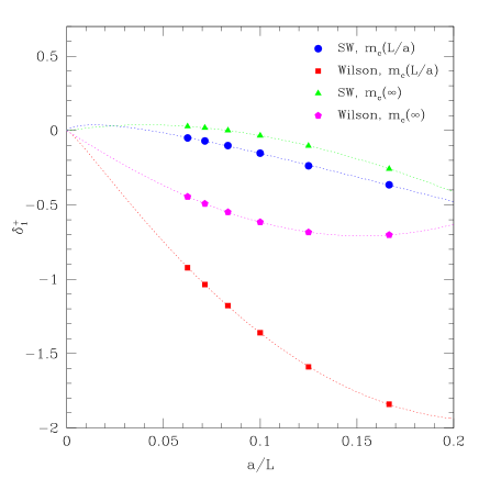
Figure 4: One-loop lattice artefacts $\delta^{+}_{1}$ and $\delta^{-}_{2}$ in the step-scaling function. The data points are obtained with the Wilson and SW actions, each for two definitions of the critical mass. The dashed lines are obtained as 4-parameter fits to the expected asymptotic behaviour and are displayed to guide the eye.

We conclude that cutoff effects in the step-scaling functions can be quite large, and the expected asymptotic dominance of linear lattice artefacts is not yet observed for our data. However, we also note that cutoff effects with the O($a$) improved action are significantly smaller, a fact that is also reflected in the non-perturbative data [?]. Moreover, for the available lattice sizes O($a^{2}$) effects seem to dominate. We take this as an indication that O($a$) improvement of the four-quark operators may be numerically unimportant, at least for the step-scaling functions considered here.

7 Conclusions

We have introduced a family of finite volume renormalization schemes for the two multiplicatively renormalizable four-quark operators in eq. (2.6). The schemes are based on the Schrödinger functional and are defined independently of a particular regularization. By matching, at one-loop order of perturbation theory, to commonly used continuum schemes (NDR, HVDR, DRED), we could infer the 2-loop anomalous operator dimensions in these SF schemes. These results are being used in a corresponding non-perturbative study [?] which completely solves the non-perturbative renormalization problem for these operators in quenched QCD. Based on this work, preliminary results for the kaon bag parameter $B_{K}$ have been presented in [?]. Besides the two multiplicatively renormalizable operators studied here, the complete basis of parity-odd four-quark operators contains eight further operators which form four pairs that mix under renormalization [?]. The study of these mixing problems both in perturbation theory and beyond is left for future work.

Acknowledgements

We thank A. Vladikas for many useful discussions and critical comments on a draft of this paper. S.S and F.P. acknowledge partial support by the cooperation CICYT-INFN 2004. C.P. thanks both the CERN Theory Division and the University of Rome “Tor Vergata” for their hospitality.

References

• [1] K. Jansen et al., Phys. Lett. B 372 (1996) 275 [arXiv:hep-lat/9512009].
• [2] M. Della Morte, R. Frezzotti, J. Heitger, J. Rolf, R. Sommer and U. Wolff [ALPHA Collaboration], arXiv:hep-lat/0411025 and references therein.
• [3] S. Sint and P. Weisz [ALPHA collaboration], Nucl. Phys. B 545 (1999) 529 [arXiv:hep-lat/9808013].
• [4] S. Capitani, M. Lüscher, R. Sommer and H. Wittig [ALPHA Collaboration], Nucl. Phys. B 544 (1999) 669 [arXiv:hep-lat/9810063].
• [5] M. Guagnelli, J. Heitger, F. Palombi, C. Pena and A. Vladikas [ALPHA Collaboration], JHEP 0405 (2004) 001 [arXiv:hep-lat/0402022].
• [6] A. Bucarelli, F. Palombi, R. Petronzio and A. Shindler, Nucl. Phys. B 552 (1999) 379 [arXiv:hep-lat/9808005].
• [7] F. Palombi, R. Petronzio and A. Shindler, Nucl. Phys. B 637 (2002) 243 [arXiv:hep-lat/0203002].
• [8] M. Guagnelli, K. Jansen, F. Palombi, R. Petronzio, A. Shindler and I. Wetzorke [Zeuthen-Rome (ZeRo) collaboration], Nucl. Phys. B 664 (2003) 276 [arXiv:hep-lat/0303012].
• [9] M. Guagnelli, K. Jansen, F. Palombi, R. Petronzio, A. Shindler and I. Wetzorke [Zeuthen-Rome (ZeRo) collaboration], arXiv:hep-lat/0405027.
• [10] M. Kurth and R. Sommer [ALPHA collaboration], Nucl. Phys. B 597 (2001) 488 [arXiv:hep-lat/0007002].
• [11] J. Heitger, M. Kurth and R. Sommer [ALPHA collaboration], Nucl. Phys. B 669 (2003) 173 [arXiv:hep-lat/0302019].
• [12] P. Dimopoulos, J. Heitger, C. Pena, S. Sint and A. Vladikas [ALPHA Collaboration], arXiv:hep-lat/0409026.
• [13] F. Palombi, C. Pena and S. Sint [ALPHA collaboration], arXiv:hep-lat/0408018.
• [14] C. Pena, S. Sint and A. Vladikas, JHEP 0409 (2004) 069 [arXiv:hep-lat/0405028].
• [15] M. Guagnelli, J. Heitger, C. Pena, S. Sint and A. Vladikas [ALPHA collaboration], Nucl. Phys. Proc. Suppl.  119 (2003) 436 [arXiv:hep-lat/0209046].
• [16] A. Donini, V. Giménez, G. Martinelli, C. T. Sachrajda, M. Talevi and A. Vladikas, Nucl. Phys. Proc. Suppl.  47 (1996) 489 [arXiv:hep-lat/9509078].
• [17] A. Donini, V. Giménez, G. Martinelli, M. Talevi and A. Vladikas, Eur. Phys. J. C 10 (1999) 121 [arXiv:hep-lat/9902030].
• [18] R. Frezzotti, P. A. Grassi, S. Sint and P. Weisz [ALPHA collaboration], JHEP 0108 (2001) 058 [arXiv:hep-lat/0101001].
• [19] D. Bećirević et al., Phys. Lett. B 487 (2000) 74 [arXiv:hep-lat/0005013].
• [20] B. Sheikholeslami and R. Wohlert, Nucl. Phys. B259 (1985) 572.
• [21] M. Lüscher, S. Sint, R. Sommer and P. Weisz, Nucl. Phys. B 478 (1996) 365 [arXiv:hep-lat/9605038].
• [22] M. Lüscher and P. Weisz, Nucl. Phys. B 479 (1996) 429 [arXiv:hep-lat/9606016].
• [23] M. Lüscher, S. Sint, R. Sommer and H. Wittig, Nucl. Phys. B 491 (1997) 344 [arXiv:hep-lat/9611015].
• [24] S. Sint and P. Weisz, Nucl. Phys. B 502 (1997) 251 [arXiv:hep-lat/9704001].
• [25] M. Lüscher, R. Narayanan, P. Weisz and U. Wolff, Nucl. Phys. B 384 (1992) 168 [arXiv:hep-lat/9207009].
• [26] S. Sint, Nucl. Phys. B 421 (1994) 135 [arXiv:hep-lat/9312079].
• [27] S. Sint, Nucl. Phys. B 451 (1995) 416 [arXiv:hep-lat/9504005].
• [28] T. van Ritbergen, J. A. M. Vermaseren and S. A. Larin, Phys. Lett. B 400 (1997) 379 [arXiv:hep-ph/9701390].
• [29] K. G. Chetyrkin, Phys. Lett. B 404 (1997) 161 [arXiv:hep-ph/9703278].
• [30] J. A. M. Vermaseren, S. A. Larin and T. van Ritbergen, Phys. Lett. B 405 (1997) 327 [arXiv:hep-ph/9703284].
• [31] M. K. Gaillard and B. W. Lee, Phys. Rev. Lett.  33 (1974) 108.
• [32] G. Altarelli and L. Maiani, Phys. Lett. B 52 (1974) 351.
• [33] G. Altarelli, G. Curci, G. Martinelli and S. Petrarca, Nucl. Phys. B 187 (1981) 461.
• [34] A. J. Buras and P. H. Weisz, Nucl. Phys. B 333 (1990) 66.
• [35] M. Ciuchini, E. Franco, V. Lubicz, G. Martinelli, I. Scimemi and L. Silvestrini, Nucl. Phys. B 523 (1998) 501 [arXiv:hep-ph/9711402].
• [36] A. J. Buras, M. Misiak and J. Urban, Nucl. Phys. B 586 (2000) 397 [arXiv:hep-ph/0005183].
• [37] W. Siegel, Phys. Lett. B 84 (1979) 193.
• [38] G. ’t Hooft and M. J. G. Veltman, Nucl. Phys. B 44 (1972) 189.
• [39] M. Lüscher, R. Sommer, P. Weisz and U. Wolff, Nucl. Phys. B 413 (1994) 481 [arXiv:hep-lat/9309005].
• [40] S. Sint and R. Sommer, Nucl. Phys. B 465 (1996) 71 [arXiv:hep-lat/9508012].
• [41] J. C. Collins, Renormalization (Cambridge Monographs on Mathematical Physics, Cambridge University Press, Cambridge 1984).
• [42] G. Martinelli, Phys. Lett. B 141 (1984) 395.
• [43] E. Gabrielli, G. Martinelli, C. Pittori, G. Heatlie and C. T. Sachrajda, Nucl. Phys. B 362 (1991) 475.
• [44] R. Frezzotti, E. Gabrielli, C. Pittori and G. C. Rossi, Nucl. Phys. B 373 (1992) 781.
• [45] G. Martinelli and Y. C. Zhang, Phys. Lett. B 123 (1983) 433 and B 125 (1983) 77.
• [46] S. Sint, private notes (1996).
• [47] H. Panagopoulos and Y. Proestos, Phys. Rev. D 65 (2002) 014511 [arXiv:hep-lat/0108021].
• [48] M. Lüscher and P. Weisz, Nucl. Phys. B 266 (1986) 309.
• [49] A. Bode, P. Weisz and U. Wolff [ALPHA collaboration], Nucl. Phys. B 576 (2000) 517 [Erratum ibid.  B600 (2001) 453,  B 608 (2001) 481] [arXiv:hep-lat/9911018].
• [50] M. Guagnelli, J. Heitger, C. Pena, S. Sint and A. Vladikas, arXiv:hep-lat/0505002.