ROM2F/2005-07

MS-TP-05-4

CERN-PH-TH/2005-044

FTUAM-05-5

IFT UAM-CSIC/05-17

May 2005

Non-perturbative renormalization of left-left

four-fermion operators in quenched lattice QCD

M. Guagnelli^a, J. Heitger^b, C. Pena^c, S. Sint^d and A. Vladikas^a

^a INFN, Sezione di Roma II

c/o Dipartimento di Fisica, Università di Roma “Tor Vergata”

Via della Ricerca Scientifica 1, I-00133 Rome, Italy

^b Westfälische Wilhelms-Universität Münster, Institut für Theoretische Physik

Wilhelm-Klemm-Strasse 9, D-48149 Münster, Germany

^c CERN, Physics Department, TH Division

CH-1211 Geneva 23, Switzerland

^d Departamento de Física Teórica C-XI and

Instituto de Física Teórica C-XVI,

Universidad Autónoma de Madrid, Cantoblanco E-28049 Madrid, Spain

 Abstract We define a family of Schrödinger Functional renormalization schemes for the four-quark multiplicatively renormalizable operators of the $\Delta F=1$ and $\Delta F=2$ effective weak Hamiltonians. Using the lattice regularization with quenched Wilson quarks, we compute non-perturbatively the renormalization group running of these operators in the continuum limit in a large range of renormalization scales. Continuum limit extrapolations are well controlled thanks to the implementation of two fermionic actions (Wilson and Clover). The ratio of the renormalization group invariant operator to its renormalized counterpart at a low energy scale, as well as the renormalization constant at this scale, is obtained for all schemes.  

1 Introduction

In the quest for accurate quantitative predictions in the non-perturbative sector of the Standard Model, non-perturbative renormalization has become an essential element of lattice QCD calculations. Two schemes are currently in use in many applications, namely the RI/MOM [1] and the Schrödinger Functional (SF) [2]. In the latter scheme the scale evolution of (matrix elements of) renormalized operators can be traced non-perturbatively over a wide range of scales. The validity of perturbation theory at high scales can thus be verified and one may then convert perturbatively to one of the commonly used continuum schemes, such as the ${\overline{\rm MS}}$ scheme of dimensional regularization. Alternatively, one may use low order perturbation theory to extrapolate from high to infinite energies, where the so-called renormalization-group-invariant (RGI) operators are defined. In any case, perturbation theory is only used in the high energy regime where it may be safely applied.

These techniques have been applied to study the scale evolution of various physical quantities, such as the QCD gauge coupling, the quark mass [3, 4, 5, 6] and the moments of pion or nucleon structure functions [7] (both in the quenched approximation and for two dynamical flavours), as well as matrix elements of the heavy-light axial current, with heavy quarks treated in the static approximation [8]. The present work is a first step towards the extension of this SF renormalization and renormalization group (RG) evolution programme to four-quark operators relevant for weak matrix elements. These arise in the OPE as the low energy QCD contribution in weak interaction transitions. They are key elements for the determination of the CKM unitarity triangle (and the subsequent understanding of CP-violation).

We specifically investigate the renormalization of two dimension-six operators with a “left-left” Dirac structure and four fermions with distinct flavours:

$$\begin{split}O_{\rm\scriptscriptstyle LL}^{\pm}(x)&=\frac{1}{2}\big{[}\left(\bar{\psi}_{1}(x)\gamma_{\mu}^{L}\psi_{2}(x)\right)\,\,\left(\bar{\psi}_{3}(x)\gamma_{\mu}^{L}\psi_{4}(x)\right)\\ &~{}~{}~{}~{}~{}~{}~{}~{}\pm\left(\bar{\psi}_{1}(x)\gamma_{\mu}^{L}\psi_{4}(x)\right)\,\,\left(\bar{\psi}_{3}(x)\gamma_{\mu}^{L}\psi_{2}(x)\right)\big{]}\\ &=O_{\rm\scriptscriptstyle VV+AA}^{\pm}-O_{\rm\scriptscriptstyle VA+AV}^{\pm}\ ,\end{split}$$ (1.1)

where $\gamma^{L}_{\mu}=\gamma_{\mu}(1-\gamma_{5})$. The last expression implicitly defines the parity-even and -odd components of $O_{\rm\scriptscriptstyle LL}^{\pm}$, in fairly standard notation. In a chirally symmetric regularization, the operators $O_{\rm\scriptscriptstyle LL}^{\pm}$ are multiplicatively renormalizable. As we opt for lattice regularizations with Wilson fermions, the loss of chiral symmetry generates extra parity-even counterterms with finite mixing coefficients. The parity-odd components $O_{\rm\scriptscriptstyle VA+AV}^{\pm}$ are protected against the generation of parity-odd counterterms by discrete symmetries. For a full account of these renormalization properties see refs. [9, 10]. In the present work we focus on these multiplicatively renormalizable, parity-odd operators $O_{\rm\scriptscriptstyle VA+AV}^{\pm}$.

Once the four generic flavours are identified with specific physical flavours, the corresponding weak matrix elements give rise to a variety of phenomenology. For example, identifying $\psi_{1}$ and $\psi_{3}$ with the strange (or bottom) quark and $\psi_{2}$ and $\psi_{4}$ with the down quark, we obtain the operator $O_{\rm\scriptscriptstyle VA+AV}^{+}$ mediating $\Delta F=2$ transitions ($K^{0}-\bar{K}^{0}$ and $B^{0}-\bar{B}^{0}$ oscillations) in the tmQCD lattice regularization framework [11]. If $\psi_{1}$ is a strange quark field and the others are suitably chosen light and charmed quarks, we are looking into $\Delta S=1$ operators $O_{\rm\scriptscriptstyle VA+AV}^{\pm}$ mediating $K\rightarrow\pi\pi$ transitions. Our results completely determine the renormalization of the operators mediating the $\Delta I=3/2$ channel, whereas for the $\Delta I=1/2$ transitions only logarithmic divergences are removed. This multiplicative renormalization is sufficient in the limit of SU(4) flavour symmetry, of which the chiral limit is a special case. Upon explicit breaking of this symmetry by the masses of the heavier quark flavours, the renormalization programme of the $\Delta I=1/2$ channel is only complete once the question of mixing with operators of lower dimension has been addressed. This mixing is beyond the scope of the current work.

The paper is organised as follows: In sect. 2 we present a general discussion on the RG running of correlation functions of composite operators, leading to the definition of the corresponding renormalization group invariant (RGI) operators. In sect. 3 we introduce the SF renormalization schemes used for the four-fermion operators in question, define the operator step scaling functions (SSF), discuss their properties and show how the operator RG running can be obtained non-perturbatively from them. In sect. 4 we present our non-perturbative computation of the SSF. Our results have been obtained in the quenched approximation. We used both the standard Wilson quark action and its $O(a)$ improved version, with the Sheikholeslami-Wohlert or clover term [12] (henceforth referred to as Clover action).Once extrapolated to the continuum limit, the SSF is used in order to obtain the ratio of the RGI operator to its renormalized counterpart at a hadronic low energy scale. In sect. 5 we compute the operator renormalization constants at this hadronic matching scale. Finally in sect. 6 we discuss our conclusions. Some technical points have been relegated to appendices. Preliminary results had already appeared in refs. [13].

In a companion paper [14] the same calculation has been performed in perturbation theory. The lattice SF schemes have been matched to a standard ${\overline{\rm MS}}$ continuum scheme, at 1-loop in perturbation theory. Combined with the known NLO results of the operator anomalous dimension in the continuum reference scheme, these results give the NLO estimate of the operator step scaling function. These in turn are used in the present work, since part of the calculation involves the RG running of the operators at very high scales in the SF schemes, where NLO perturbation theory may be safely applied.

2 Callan-Symanzik equations and RGI operators

Our starting point is the Callan-Symanzik equation expressing the RG running of correlation functions under a change of renormalization scale $\mu$. Our exposition and notation follows closely that of Refs. [4, 15]. We first consider an arbitrary bare $n$-point correlation function

$$\begin{split}G(x_{1},\ldots,x_{n};g_{0},m_{0,{\rm f}})&=\langle O_{1}(x_{1})\cdots O_{n}(x_{n})\rangle\\ &={\cal Z}^{-1}\int{\cal D}[\psi,\bar{\psi}]{\cal D}[U]e^{-S}O_{1}(x_{1})\cdots O_{n}(x_{n})\ ,\end{split}$$ (2.2)

where the $O_{i}$ are local gauge invariant composite operators and ${\cal Z}$ is the QCD partition function. A regularization such as the lattice (with ultraviolet cutoff $a^{-1}$) is implied. For simplicity we assume that all space-time points are separated; i.e. $x_{i}\neq x_{j}$ for $i\neq j;~{}i,j=1,\ldots,n$. The dependence on the bare parameters $g_{0},m_{0,{\rm f}}$ of the theory has been indicated explicitly. As this is quite cumbersome, occasionally we will omit some of the arguments, in order to simplify the notation. The subscript ${\rm f}=1,\ldots,N_{f}$ borne by the mass indicates flavour (the mass matrix will be henceforth assumed to be diagonal).

It is adequate for the purposes of the present work to consider only multiplicatively renormalized operators (i.e. no operator mixing occurs). Their renormalized correlation functions at scale $\mu$ can be written as

$$G_{\rm R}(x_{1},\ldots,x_{n};\mu,g_{\rm R},m_{{\rm R},\rm f})=\left[\prod_{i=1}^{n}Z_{O_{i}}(g_{0},a\mu)\right]G(x_{1},\ldots,x_{n};g_{0},m_{0,{\rm f}})\ .$$ (2.3)

We denote the renormalized coupling by $g_{\rm R}$ and the renormalized quark masses by $m_{{\rm R},\rm f}$. The operator renormalization constants $Z_{O_{i}}$ are determined by imposing $n$ renormalization conditions on suitably chosen correlation functions of the operators $O_{i}(x)$, at scale $\mu$. In the context of the present discussion these conditions need not be specified; it is crucial however to keep in mind that they are imposed in the chiral limit [16], i.e. we are only considering mass independent renormalization schemes.

The correlation function defined in eq. (2.3) fulfills a Callan-Symanzik equation which determines the RG running of the operator in question:

$$\left[\mu\frac{\partial}{\partial\mu}+\beta(g_{\rm R})\frac{\partial}{\partial g_{\rm R}}+\tau(g_{\rm R})\sum_{{\rm f}=1}^{N_{f}}m_{{\rm R},\rm f}\frac{\partial}{\partial m_{{\rm R},\rm f}}-\sum_{i=1}^{n}\gamma_{O_{i}}(g_{\rm R})\right]G_{\rm R}=\mbox{O}(a)\ ,$$ (2.4)

where $\beta(g_{\rm R})$ in the Callan-Symanzik function, $\tau(g_{\rm R})$ the quark mass anomalous dimension and $\gamma_{O_{i}}(g_{\rm R})$ the anomalous dimension of operator $O_{i}$, which is related to its renormalization constant through

$$\gamma_{O}(\kern 1.0pt\overline{\kern-1.0ptg\kern 0.0pt}\kern 1.0pt(\mu))=\lim_{a\to 0}\left(\mu\frac{\partial}{\partial\mu}Z_{O}(g_{0},a\mu)\right)Z_{O}(g_{0},a\mu)^{-1}\ .$$ (2.5)

Since the renormalization scheme we are working in is mass independent, $\beta$, $\tau$ and $\gamma_{O}$ depend only on the renormalized coupling. Their asymptotic expansions at small values of the coupling are given by

$$\beta(g) \stackrel{{\scriptstyle g\to 0}}{{\sim}}-g^{3}\left(b_{0}+b_{1}g^{2}+b_{2}g^{4}+\ldots\right)\ ,$$ (2.6)

$$\tau(g) \stackrel{{\scriptstyle g\to 0}}{{\sim}}-g^{2}\left(d_{0}+d_{1}g^{2}+d_{2}g^{4}+\ldots\right)\ ,$$ (2.7)

$$\gamma_{O}(g) \stackrel{{\scriptstyle g\to 0}}{{\sim}}-g^{2}\left(\gamma_{O}^{(0)}+\gamma_{O}^{(1)}g^{2}+\gamma_{O}^{(2)}g^{4}+\ldots\right)\ .$$ (2.8)

Running parameters are then defined as usual:

$$q\frac{\partial\kern 1.0pt\overline{\kern-1.0ptg\kern 0.0pt}\kern 1.0pt}{\partial q}=\beta(\kern 1.0pt\overline{\kern-1.0ptg\kern 0.0pt}\kern 1.0pt(q)),~{}~{}~{}~{}~{}~{}~{}q\frac{\partial\kern 2.0pt\overline{\kern-1.0ptm\kern-1.0pt}\kern 1.0pt_{\rm f}}{\partial q}=\tau(\kern 1.0pt\overline{\kern-1.0ptg\kern 0.0pt}\kern 1.0pt(q))\,\,\kern 2.0pt\overline{\kern-1.0ptm\kern-1.0pt}\kern 1.0pt_{\rm f}(q)\ ,$$ (2.9)

supplemented by the boundary conditions

$$\kern 1.0pt\overline{\kern-1.0ptg\kern 0.0pt}\kern 1.0pt(\mu)=g_{\rm R},~{}~{}~{}~{}~{}~{}~{}\kern 2.0pt\overline{\kern-1.0ptm\kern-1.0pt}\kern 1.0pt_{\rm f}(\mu)=m_{{\rm R},\rm f}\ .$$ (2.10)

To define RGI composite operators, we start with the formal integration of eq. (2.4), yielding

$$\begin{split}G_{\rm R}(x_{1},\ldots,x_{n};\mu^{\prime},\kern 1.0pt\overline{\kern-1.0ptg\kern 0.0pt}\kern 1.0pt(\mu^{\prime}),\kern 2.0pt\overline{\kern-1.0ptm\kern-1.0pt}\kern 1.0pt_{\rm f}(\mu^{\prime}))&=\\ =\Big{[}\prod_{i=1}^{n}U_{i}(\mu^{\prime},\mu)\Big{]}G_{\rm R}&(x_{1},\ldots,x_{n};\mu,\kern 1.0pt\overline{\kern-1.0ptg\kern 0.0pt}\kern 1.0pt(\mu),\kern 2.0pt\overline{\kern-1.0ptm\kern-1.0pt}\kern 1.0pt_{\rm f}(\mu))+\mbox{O}(a)\ ,\end{split}$$ (2.11)

where $U_{i}$ is the evolution function

$$U_{i}(\mu^{\prime},\mu)=\exp\left\{\int_{\kern 1.0pt\overline{\kern-1.0ptg\kern 0.0pt}\kern 1.0pt(\mu)}^{\kern 1.0pt\overline{\kern-1.0ptg\kern 0.0pt}\kern 1.0pt(\mu^{\prime})}\frac{\gamma_{O_{i}}(g)}{\beta(g)}{\rm d}g\right\}\ .$$ (2.12)

This function describes the RG evolution in the continuum limit of the renormalized operator $(O_{i})_{\rm R}$ between the renormalization point $\mu$ and an arbitrary scale $\mu^{\prime}$, namely:

$$(O_{i})_{\rm R}(x;\mu^{\prime})=U_{i}(\mu^{\prime},\mu)\,\,(O_{i})_{\rm R}(x;\mu)\ .$$ (2.13)

It can easily be seen to satisfy the RG equation

$$q\frac{\partial U_{i}(q,\mu)}{\partial q}=\gamma_{O}(\kern 1.0pt\overline{\kern-1.0ptg\kern 0.0pt}\kern 1.0pt(q))U_{i}(q,\mu)$$ (2.14)

with initial condition

$$U_{i}(\mu,\mu)=1\ .$$ (2.15)

From eqs. (2.3) and eq. (2.11) we can also express it as a ratio of renormalization constants

$$U_{i}(\mu^{\prime},\mu)=\lim_{a\to 0}\frac{Z_{O_{i}}(g_{0},a\mu^{\prime})}{Z_{O_{i}}(g_{0},a\mu)}\ .$$ (2.16)

The RGI operator could in principle be obtained by splitting the r.h.s. of eq. (2.12) into two integrals (one from $\kern 1.0pt\overline{\kern-1.0ptg\kern 0.0pt}\kern 1.0pt(\mu^{\prime})$ to $\kern 1.0pt\overline{\kern-1.0ptg\kern 0.0pt}\kern 1.0pt=0$ and one from $\kern 1.0pt\overline{\kern-1.0ptg\kern 0.0pt}\kern 1.0pt=0$ to $\kern 1.0pt\overline{\kern-1.0ptg\kern 0.0pt}\kern 1.0pt(\mu)$) and subsequently bringing the $\mu$-dependent integral on the l.h.s. of eq. (2.13). The problem is that $U_{i}(\mu^{\prime},\mu)$ diverges logarithmically in the limit $\mu^{\prime}\to\infty$. This is most clearly seen upon considering the asymptotic expansions admitted by $\beta$ (cf. eq. (2.6)) and $\gamma_{O}$ (cf. eq. (2.8)) at small values of the coupling. Hence, we proceed by casting eq. (2.13) in the form

$$\begin{split}\bigg{[}\frac{\kern 1.0pt\overline{\kern-1.0ptg\kern 0.0pt}\kern 1.0pt^{2}(\mu^{\prime})}{4\pi}\bigg{]}^{-\gamma_{O}^{(0)}/(2b_{0})}O_{\rm R}(x;\mu^{\prime})&=\bigg{[}\frac{\kern 1.0pt\overline{\kern-1.0ptg\kern 0.0pt}\kern 1.0pt^{2}(\mu)}{4\pi}\bigg{]}^{-\gamma_{O}^{(0)}/(2b_{0})}\times\\ \times\exp&\left\{-\int_{\kern 1.0pt\overline{\kern-1.0ptg\kern 0.0pt}\kern 1.0pt(\mu^{\prime})}^{\kern 1.0pt\overline{\kern-1.0ptg\kern 0.0pt}\kern 1.0pt(\mu)}{{\rm d}g}\bigg{(}\frac{\gamma_{O}(g)}{\beta(g)}-\frac{\gamma_{O}^{(0)}}{b_{0}g}\bigg{)}\right\}O_{\rm R}(x;\mu)\,.\\ \end{split}$$ (2.17)

What has been achieved is the finiteness of the r.h.s. of eq. (LABEL:towards_genRGI_2) as $\mu^{\prime}\to\infty$ (i.e. $\kern 1.0pt\overline{\kern-1.0ptg\kern 0.0pt}\kern 1.0pt(\mu^{\prime})\to 0$) for any value of $\mu$. Moreover, since there is no $\mu$-dependence on the l.h.s., also the r.h.s. is $\mu$-independent. Hence, taking the limit $\mu^{\prime}\to\infty$ of eq. (LABEL:towards_genRGI_2), we define a RGI quantity as

$$\hat{O}(x)=\hat{Z}_{O}(\mu)O_{\rm R}(x;\mu)\ ,$$ (2.18)

where we have introduced

$$\hat{Z}_{O}(\mu)=\bigg{[}\frac{\kern 1.0pt\overline{\kern-1.0ptg\kern 0.0pt}\kern 1.0pt^{2}(\mu)}{4\pi}\bigg{]}^{-\gamma_{O}^{(0)}/(2b_{0})}\exp\left\{-\int_{0}^{\kern 1.0pt\overline{\kern-1.0ptg\kern 0.0pt}\kern 1.0pt(\mu)}{{\rm d}g}\bigg{(}\frac{\gamma_{O}(g)}{\beta(g)}-\frac{\gamma_{O}^{(0)}}{b_{0}g}\bigg{)}\right\}\ .$$ (2.19)

It must be stressed that the RGI operator $\hat{O}(x)$ defined above is (unlike $O_{\rm R}(x;\mu)$) independent of the renormalization scheme and scale. The expressions (2.18) and (2.19) for $\hat{O}(x)$ are an exact result, in close analogy to the ones reported in ref. [4] for the RGI quark mass

$$M_{\rm f}=\kern 2.0pt\overline{\kern-1.0ptm\kern-1.0pt}\kern 1.0pt_{\rm f}(\mu)\left(2b_{0}\kern 1.0pt\overline{\kern-1.0ptg\kern 0.0pt}\kern 1.0pt^{2}(\mu)\right)^{-d_{0}/(2b_{0})}\exp\left\{-\int_{0}^{\kern 1.0pt\overline{\kern-1.0ptg\kern 0.0pt}\kern 1.0pt(\mu)}{{\rm d}g}\bigg{(}\frac{\tau(g)}{\beta(g)}-\frac{d_{0}}{b_{0}g}\bigg{)}\right\}\,,$$ (2.20)

and the RGI scale

$$\begin{split}\Lambda=\mu&\left(b_{0}\kern 1.0pt\overline{\kern-1.0ptg\kern 0.0pt}\kern 1.0pt^{2}(\mu)\right)^{-b_{1}/(2b_{0}^{2})}\exp\left\{-\frac{1}{2b_{0}\kern 1.0pt\overline{\kern-1.0ptg\kern 0.0pt}\kern 1.0pt^{2}(\mu)}\right\}\times\\ &\times\exp\left\{-\int_{0}^{\kern 1.0pt\overline{\kern-1.0ptg\kern 0.0pt}\kern 1.0pt(\mu)}{{\rm d}g}\bigg{(}\frac{1}{\beta(g)}+\frac{1}{b_{0}g^{3}}-\frac{b_{1}}{b_{0}^{2}g}\bigg{)}\right\}\,.\end{split}$$ (2.21)

Notice that the only arbitrariness in the definition of these RGI quantities is a constant overall normalization factor. For composite operators in Eq. (2.18) we have adopted the normalization usually employed in the definition of the RGI kaon mixing parameter $\hat{B}_{K}$.

3 RG running of four-fermion operators

Having exposed the general principles for the RG behaviour of multiplicatively renormalizable composite operators, we now pass to the specific case of interest. This refers to the dimension-six composite operators of four distinct quark flavours

$$\begin{split}O_{\rm\scriptscriptstyle VA+AV}^{\pm}(x)=&\frac{1}{2}\big{\{}\big{[}(\bar{\psi}_{1}\gamma_{\mu}\psi_{2})(\bar{\psi}_{3}\gamma_{\mu}\gamma_{5}\psi_{4})+(\bar{\psi}_{1}\gamma_{\mu}\gamma_{5}\psi_{2})(\bar{\psi}_{3}\gamma_{\mu}\psi_{4})\big{]}\\ &\pm\big{[}(\bar{\psi}_{1}\gamma_{\mu}\psi_{4})(\bar{\psi}_{3}\gamma_{\mu}\gamma_{5}\psi_{2})+(\bar{\psi}_{1}\gamma_{\mu}\gamma_{5}\psi_{4})(\bar{\psi}_{3}\gamma_{\mu}\psi_{2})\big{]}\big{\}}\,,\end{split}$$ (3.22)

which are known to be multiplicatively renormalizable [9, 10]. In this section we define the correlation functions of interest, the renormalization conditions imposed and the step scaling functions of the operators $O_{\rm\scriptscriptstyle VA+AV}^{\pm}$.

As anticipated, we opt for the lattice Schrödinger functional (SF) formalism [17, 18, 19]. We regularize QCD on a lattice of extension $L^{3}\times T$ (here $T=L$ always) with periodic boundary conditions in the space directions (up to a phase $\theta$ for the fermion fields) and Dirichlet boundary conditions in the Euclidean time direction [18, 19]. Otherwise the lattice gauge and fermionic field actions are of the standard Wilson type; the Clover $\mbox{O}(a)$ improved version of the fermionic action is also used. The operators $O_{\rm\scriptscriptstyle VA+AV}^{\pm}(x)$ are defined locally on the lattice; i.e. all quark fields live at the point $x$.

The paper follows closely the notation of ref. [20], to which the reader is referred for unexplained notation.

3.1 Schrödinger Functional correlation functions

Bare composite operators are defined at both time boundaries in terms of the boundary fields $\zeta$ and $\zeta^{\prime}$ of refs. [19, 20, 21],

$$\begin{split}{\cal O}_{12}[\Gamma]&=a^{6}\sum_{\mathbf{x},\mathbf{y}}\bar{\zeta}_{1}(\mathbf{x})\Gamma\zeta_{2}(\mathbf{y})\,,\\ {\cal O}^{\prime}_{12}[\Gamma]&=a^{6}\sum_{\mathbf{x},\mathbf{y}}\bar{\zeta}^{\prime}_{1}(\mathbf{x})\Gamma\zeta^{\prime}_{2}(\mathbf{y})\,.\end{split}$$ (3.23)

The indices 1,2 label distinct flavours. Unprimed fields are defined on the $x_{0}=0$ boundary, primed ones on the $x_{0}=T$ one. There are two allowed independent choices for the Dirac matrices, namely $\Gamma=\gamma_{5}$ and $\Gamma=\gamma_{k}$ (with $k=1,2,3$). This is due to the SF Dirichlet boundary conditions of the quark fields, which involve positive and negative projection operators $P_{\pm}={\scriptstyle{{1\over 2}}}(1\pm\gamma_{0})$ [21]. The presence of these projectors implies that boundary sources with other Dirac matrices $\Gamma$ either vanish or are identical to those with $\gamma_{5}$ or $\gamma_{k}$.

The bare correlation functions of the four-fermion operators are now chosen as follows:

$${\cal F}^{\pm}_{[\Gamma_{\rm A},\Gamma_{\rm B},\Gamma_{\rm C}]}(x_{0})=\frac{1}{L^{3}}\langle{\cal O}_{21}[\Gamma_{\rm A}]{\cal O}_{45}[\Gamma_{\rm B}]\,\,\,O_{\rm\scriptscriptstyle VA+AV}^{\pm}(x)\,\,\,{\cal O}^{\prime}_{53}[\Gamma_{\rm C}]\rangle\,.$$ (3.24)

These are depicted, in terms of valence quark lines, in Fig. 1. Since the boundary operators defined in eqs. (3.23) involve sums over all 3-space at each time boundary, translational invariance implies that the above correlation functions depend only on time. A few words are in place in order to motivate the choice of this rather complicated quantity, involving three composite operators at the boundary. As stated above, the boundary operators can either be ${\cal O}_{12}[\gamma_{5}]$ or ${\cal O}_{12}[\gamma_{k}]$ (and ${\cal O}^{\prime}_{12}[\gamma_{5}]$, ${\cal O}^{\prime}_{12}[\gamma_{k}]$). Moreover, the bulk operators $O_{\rm\scriptscriptstyle VA+AV}^{\pm}(x)$ are parity-odd. These facts, combined with the requirement that cubic symmetry be respected by the correlation functions, give as simplest possibilities the following five, in principle independent correlation functions:

$$\begin{split}F^{\pm}_{1}(x_{0})&={\cal F}^{\pm}_{[\gamma_{5},\gamma_{5},\gamma_{5}]}(x_{0})\,,\\ F^{\pm}_{2}(x_{0})&=\frac{1}{6}\sum_{j,k,l=1}^{3}\epsilon_{jkl}{\cal F}^{\pm}_{[\gamma_{j},\gamma_{k},\gamma_{l}]}(x_{0})\,,\\ F^{\pm}_{3}(x_{0})&=\frac{1}{3}\sum_{k=1}^{3}{\cal F}^{\pm}_{[\gamma_{5},\gamma_{k},\gamma_{k}]}(x_{0})\,,\\ F^{\pm}_{4}(x_{0})&=\frac{1}{3}\sum_{k=1}^{3}{\cal F}^{\pm}_{[\gamma_{k},\gamma_{5},\gamma_{k}]}(x_{0})\,,\\ F^{\pm}_{5}(x_{0})&=\frac{1}{3}\sum_{k=1}^{3}{\cal F}^{\pm}_{[\gamma_{k},\gamma_{k},\gamma_{5}]}(x_{0})\,.\end{split}$$ (3.25)

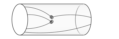
Figure 1: Four-fermion correlation functions in a finite spacetime volume with Schrödinger Functional boundary conditions. The lines denote valence quark propagation of different flavours; the double dots in the bulk denote the four-fermion operator.

We will also need the boundary-to-boundary correlation functions

$$\begin{split}f_{1}&=-\frac{1}{2L^{6}}\langle{\cal O}^{\prime}_{12}[\gamma_{5}]\,\,\,{\cal O}_{21}[\gamma_{5}]\rangle\,,\\ k_{1}&=-\frac{1}{6L^{6}}\sum_{k=1}^{3}\langle{\cal O}^{\prime}_{12}[\gamma_{k}]\,\,\,{\cal O}_{21}[\gamma_{k}]\rangle\,.\end{split}$$ (3.26)

In terms of valence quark propagators, these correlation functions are depicted in Fig. 2.

In practical simulations, these correlation functions are computed as traces of the boundary-to-bulk valence quark propagators $H_{\rm f}(x)$ and $H^{\prime}_{\rm f}(x)$, defined in ref. [22].

3.2 Schrödinger Functional renormalization schemes

Before turning to the renormalization of four-fermion operators, we recall that SF renormalization schemes are mass independent; i.e. renormalization is performed in the chiral limit. The renormalization scale is set at $\mu=1/L$; the renormalized coupling $\kern 1.0pt\overline{\kern-1.0ptg\kern 0.0pt}\kern 1.0pt(1/L)$ (defined in ref. [3]) and quark mass $\kern 2.0pt\overline{\kern-1.0ptm\kern-1.0pt}\kern 1.0pt(1/L)$ (defined in refs. [4, 15]) are then only functions of this scale.

Upon removing the ultraviolet cutoff (i.e. $a\rightarrow 0$), the bare correlation functions defined in eqs. (3.24, 3.26) diverge logarithmically. The divergence due to the boundary fields is removed by considering suitable ratios of correlation functions. Several choices can be made, giving rise to different correlator ratios. In the present work we will be considering the following nine specific cases

$$\begin{split}h^{\pm}_{\rm i}(x_{0})=\frac{F^{\pm}_{\rm i}(x_{0})}{f_{1}^{3/2}}&\qquad{\rm i}=1,\dots,5\ ,\\ h^{\pm}_{6}(x_{0})=\frac{F^{\pm}_{2}(x_{0})}{k_{1}^{3/2}}&\ ,\\ h^{\pm}_{{\rm i}+4}(x_{0})=\frac{F^{\pm}_{\rm i}(x_{0})}{f_{1}^{1/2}k_{1}}&\qquad{\rm i}=3,4,5\ ,\end{split}$$ (3.27)

which renormalize as the four-fermion operators $O_{\rm\scriptscriptstyle VA+AV}^{\pm}$ themselves:

$$h^{\pm}_{\rm R;s}(x_{0};\mu)=Z_{\rm\scriptscriptstyle VA+AV;{\rm s}}^{\pm}(g_{0},a\mu)h^{\pm}_{\rm s}(x_{0};g_{0})\qquad{\rm s}=1,\ldots,9\ .$$ (3.28)

The above renormalization constants are fixed by imposing the following renormalization conditions on the correlator $h^{\pm}_{\rm s}$ on time-slice $x_{0}=L/2$ (for all ${\rm s}=1,\dots,9$) at scale $\mu=1/L$ and fixed renormalized coupling $\kern 1.0pt\overline{\kern-1.0ptg\kern 0.0pt}\kern 1.0pt^{2}(1/L)=u$ in the chiral limit:

$$Z_{\rm\scriptscriptstyle VA+AV;{\rm s}}^{\pm}(g_{0},a\mu)h^{\pm}_{\rm s}(x_{0};g_{0})=h^{\pm}_{\rm s}(x_{0};g_{0})\bigg{|}_{g_{0}=0}\,\,;$$ (3.29)

i.e. at tree level $Z_{\rm\scriptscriptstyle VA+AV;s}^{\pm}=1$ by construction. We will always impose eq. (3.29) at $\theta=0.5$ [4, 15]. The nine correlator ratios chosen above give rise to nine in principle distinct SF renormalization schemes for each of the two operators.

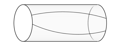
Figure 2: Boundary-to-boundary correlation function in a finite spacetime volume with Schrödinger Functional boundary conditions. The lines denote valence quark propagation of different flavours.

The above construction hinges on a theory of five flavours, the fifth one being a spectator quark. This, however, is only apparent. As already mentioned in the introduction, we make contact with a specific weak matrix element by judiciously attributing specific physical flavour labels to the above five nominal flavours. For example, the identifications

$$\psi_{1}=\psi_{3}=s\,,\qquad\psi_{2}=\psi_{4}=d\,,\qquad\psi_{5}=u$$ (3.30)

lead (up to an irrelevant factor of 2 arising from a doubling of Wick contractions) to the renormalization of the “left-left” operator $O_{\rm\scriptscriptstyle VA+AV}^{+}$, which mediates $\Delta S=2$ transitions.

3.3 Step scaling functions

The step scaling functions (SSF) of the four-fermion operators of eq. (3.22) are defined as

$$\Sigma_{\rm\scriptscriptstyle VA+AV;s}^{\pm}(u,a/L)=\frac{Z_{\rm\scriptscriptstyle VA+AV;{\rm s}}^{\pm}(g_{0},a/2L)}{Z_{\rm\scriptscriptstyle VA+AV;{\rm s}}^{\pm}(g_{0},a/L)}\Bigg{|}_{m=0,~{}\kern 1.0pt\overline{\kern-1.0ptg\kern 0.0pt}\kern 1.0pt^{2}(1/L)=u}\,\,.$$ (3.31)

This is in close analogy to the quark mass case [4]; i.e. $\Sigma_{\rm\scriptscriptstyle VA+AV;s}^{\pm}$ is defined in the chiral limit $m(g_{0})=0$, for a lattice of a given resolution $L/a$ and at fixed renormalized coupling $\kern 1.0pt\overline{\kern-1.0ptg\kern 0.0pt}\kern 1.0pt^{2}(1/L)=u$. The precise definition of the current quark mass $m(g_{0})$ can be found in ref. [4]. The lattice SSF $\Sigma_{\rm\scriptscriptstyle VA+AV;s}^{\pm}$ is not unique: it depends on the details of the lattice regularization (e.g. the type of lattice action chosen, the level of $\mbox{O}(a)$ improvement etc.). It has, however, a well defined continuum limit, which should be unique (i.e. universality should hold). We denote the continuum SSF by

$$\sigma_{\rm\scriptscriptstyle VA+AV;s}^{\pm}(u)=\lim_{a\to 0}\Sigma_{\rm\scriptscriptstyle VA+AV;s}^{\pm}(u,a/L)\,\,.$$ (3.32)

In terms of the operators’ evolution function $U_{\rm\scriptscriptstyle VA+AV;s}^{\pm}$ and anomalous dimension $\gamma_{\rm\scriptscriptstyle VA+AV;s}^{\pm}$ the SSF can be written as (cf. eqs. (2.12,2.16))

$$\sigma_{\rm\scriptscriptstyle VA+AV;s}^{\pm}(u)=U_{\rm\scriptscriptstyle VA+AV;s}^{\pm}\Big{(}\frac{1}{2L},\frac{1}{L}\Big{)}=\exp\left\{\int_{\kern 1.0pt\overline{\kern-1.0ptg\kern 0.0pt}\kern 1.0pt(1/L)}^{\kern 1.0pt\overline{\kern-1.0ptg\kern 0.0pt}\kern 1.0pt(1/2L)}\frac{\gamma_{\rm\scriptscriptstyle VA+AV;s}^{\pm}(g)}{\beta(g)}\,{\rm d}g\right\}\,.$$ (3.33)

Thus the physical meaning of $\sigma_{\rm\scriptscriptstyle VA+AV;s}^{\pm}$ emerges readily from the above as the operator evolution function between two scales differing by a factor of 2. It is a quantity closely related to the anomalous dimension of the corresponding operator.

We stress that the operator anomalous dimension is scheme dependent. Its perturbative expansion is known to two-loop order; the universal one-loop coefficient is

$$\gamma_{\rm\scriptscriptstyle VA+AV}^{\pm(0)}=\pm\frac{1}{(4\pi)^{2}}\frac{6(N\mp 1)}{N}\,,$$ (3.34)

($N$ being the number of colours) while the two-loop coefficients $\gamma_{\rm\scriptscriptstyle VA+AV;s}^{\pm(1)}$ have been calculated in [14] for the schemes defined by eqs. (3.29).

Finally, from eq. (2.19) we immediately obtain the following expression for the factor relating the renormalized operator at a scale $\mu$ with its RGI counterpart:

$$\begin{split}\hat{Z}_{\rm VA+AV;s}^{\pm}(\mu)=\bigg{[}\frac{\kern 1.0pt\overline{\kern-1.0ptg\kern 0.0pt}\kern 1.0pt^{2}(\mu)}{4\pi}\bigg{]}^{-\gamma_{\rm\scriptscriptstyle VA+AV}^{\pm(0)}/(2b_{0})}&\times\\ \times\exp\bigg{\{}-\int_{0}^{\kern 1.0pt\overline{\kern-1.0ptg\kern 0.0pt}\kern 1.0pt(\mu)}&{{\rm d}g}\bigg{(}\frac{\gamma_{\rm\scriptscriptstyle VA+AV;s}^{\pm}(g)}{\beta(g)}-\frac{\gamma_{\rm\scriptscriptstyle VA+AV;s}^{\pm(0)}}{b_{0}g}\bigg{)}\bigg{\}}\,.\end{split}$$ (3.35)

It is the aim of the present work to provide accurate estimates of the above quantity in all nine schemes and for a large range of scales $\mu=1/L$ (albeit in the quenched approximation).

It is useful to keep in mind that the only flavour dependence of $\hat{Z}_{\rm VA+AV;s}^{\pm}(\mu)$ is through $N_{f}$; there is no dependence on the values of the physical quark masses, as this quantity in defined (and computed) in the chiral limit. Thus it can be readily used in the renormalization of various physical matrix elements.

3.4 RG running of four-fermion operators

Once the step scaling functions $\sigma_{\rm\scriptscriptstyle VA+AV;s}^{\pm}$ have been computed through numerical simulation, the ratio of renormalized correlation functions involving the four-fermion operators of interest between the minimum and maximum renormalization scales covered by these simulations can be worked out. In order to be consistent with the notation of ref. [4], we denote the former by $\mu_{\rm min}=(2L_{\rm max})^{-1}$. The ratio in question is then obtained in two steps:

First the SSF of the gauge coupling

$$\sigma(u)=\left.\kern 1.0pt\overline{\kern-1.0ptg\kern 0.0pt}\kern 1.0pt^{2}(1/2L)\right|_{\kern 1.0pt\overline{\kern-1.0ptg\kern 0.0pt}\kern 1.0pt^{2}(1/L)=u}\ ,$$ (3.36)

computed in [3, 4], is used in order to determine the correspondence between renormalized couplings and renormalization scales. This is done through the recursion

$$u_{l}=\sigma(u_{l+1})\,,$$ (3.37)

with $u_{0}=\kern 1.0pt\overline{\kern-1.0ptg\kern 0.0pt}\kern 1.0pt^{2}(1/L_{\rm max})=3.48$ the initial value.

Second the SSF $\sigma_{\rm\scriptscriptstyle VA+AV;s}^{\pm}$, known non-perturbatively, is used for this sequence of couplings in order to compute the quantity

$$U_{\rm\scriptscriptstyle VA+AV;s}^{\pm}(\mu_{\rm min},2^{k}\mu_{\rm min})=\prod_{l=0}^{k-1}\left[\sigma_{\rm\scriptscriptstyle VA+AV;{\rm s}}^{\pm}(u_{l})\right]\,.$$ (3.38)

The number of recursion steps $k$ has to be chosen so that the (large) scale $2^{k}\mu_{\rm min}$ lies in the range covered by the computation of the SSF. In practice (cf. section 4), it is safe to take $k=7$, which means that $2^{k}\mu_{\rm min}$ is deep in the region where perturbation theory can be expected to apply.

The final step in our calculation is the computation of the RG running factor of eq. (3.35) at the renormalization point $\mu_{\rm min}$, written as a product:

$$\hat{Z}_{\rm VA+AV;s}^{\pm}(\mu_{\rm min})=U_{\rm\scriptscriptstyle VA+AV;s}^{\pm}(2^{k}\mu_{\rm min},\mu_{\rm min})\hat{Z}_{\rm VA+AV;s}^{\pm}(2^{k}\mu_{\rm min})\ .$$ (3.39)

The first factor on the r.h.s. is known from eq. (3.38). The second factor, which involves a (presumably) perturbative scale $2^{k}\mu_{\rm min}$, is calculated from eq. (3.35) with the NNLO and NLO perturbative expressions of $\beta(g)$ and $\gamma_{\rm\scriptscriptstyle VA+AV;s}^{\pm}(g)$, respectively. Clearly the underlying assumption is that the truncation of the perturbative series at NLO is safe at this scale. This is a scheme dependent statement. The perturbative results of ref. [14] indicate that, for schemes $s=1,3,7$, the NLO coefficient of $\gamma_{\rm\scriptscriptstyle VA+AV;s}^{+}$ is of the same sign and much smaller than the LO one; $s=1$ is the scheme with the smallest NLO coefficient. In all other schemes the relative sign is negative. For $\gamma_{\rm\scriptscriptstyle VA+AV;s}^{-}$ the ratio is negative for all nine schemes, with $s=8$ the smallest in absolute value. Conservatively, we indicate $s=1$ and $s=8$ as the most suitable schemes for operators $O_{\rm\scriptscriptstyle VA+AV}^{+}$ and $O_{\rm\scriptscriptstyle VA+AV}^{-}$ respectively. We stress that these choices are only dictated by the behaviour of the NLO perturbative results; the non-perturbative computation is equally reliable for all nine schemes considered. In any case, we have carried out our computations for all schemes.

4 Non-perturbative computation of the step scaling function

In this section we present the computation of $\Sigma_{\rm\scriptscriptstyle VA+AV;s}^{\pm}$ and its extrapolation to the continuum limit. We also obtain estimates of the corresponding RGI quantity (or, more precisely, of the expression of eq. (3.39) at a hadronic scale). The method of computation parallels closely that of refs. [4, 5] for the SSF of the quark mass $\Sigma_{\rm\scriptscriptstyle P}$.

4.1 Wilson and Clover actions

We have used both the standard Wilson action and its $\mbox{O}(a)$ improved version (Clover) in our simulations. Our notation is fairly standard; $\beta\equiv 6/g_{0}^{2}$ is the inverse coupling and $\kappa\equiv 1/[2am_{0}+8]$ is the hopping parameter. At fixed bare coupling we define $\kappa_{\rm cr}$ as the value where the PCAC quark mass $m(g_{0})$ of ref. [4] vanishes. Following [4], the computation of $\kappa_{\rm cr}$ is done at $\theta=0$.

The $\mbox{O}(a)$ Symanzik improvement of the Schrödinger Functional has been worked out in refs. [18, 20, 12]. For the pure gauge action, it amounts to modifying it by introducing time-boundary counterterms proportional to $[c_{\rm t}(g_{0}^{2})-1]$. For the fermionic action we must introduce the well-known clover counterterm in the lattice bulk, proportional to $c_{\rm sw}(g_{0}^{2})$, and time-boundary counterterms proportional to $[\tilde{c}_{\rm t}(g_{0}^{2})-1]$. Correlation functions of composite operators may then also be $\mbox{O}(a)$ improved by including in their lattice definition the appropriate higher dimension counterterms. Since for dimension-six operators, such as the ones of eq. (3.22), there are several dimension-seven counterterms, we will not pursue operator improvement in this work.

The improvement coefficient $c_{\rm sw}$ has been computed non-perturbatively for a range of values of the bare coupling $g_{0}$; see ref. [26]. The coefficients $c_{\rm t}$ and $\tilde{c}_{\rm t}$ are known only in perturbation theory, to NLO [27] and LO [21] respectively:

$$c_{\rm t}(g_{0}^{2}) =1-0.089g_{0}^{2}-0.030g_{0}^{4}\,\,,$$ (4.40)

$$\tilde{c}_{\rm t}(g_{0}^{2}) =1-0.018g_{0}^{2}\,.$$ (4.41)

In the present work we will distinguish two approaches to the continuum limit:

1. What we call “Wilson action results” (or “Wilson case” for short) consists in setting $c_{\rm sw}=0\,\,$. Moreover, we set $\tilde{c}_{\rm t}=1$, while the one-loop value (eq. (4.40) truncated to O($g_{0}^{2}$)) is used for $c_{\rm t}$.

2. What we call “Clover action results” (or “Clover case” for short) consists in using the Clover action with a non-perturbative $c_{\rm sw}$. The one-loop value from eqs. (4.40) and (4.41) is used for $c_{\rm t}$ and $\tilde{c}_{\rm t}$ respectively.

In both cases the four-fermion operator is left unimproved, so the dominant discretisation effects are expected to be $\mbox{O}(a)$. We note, however, that the correlation functions (3.25) are $\mbox{O}(a)$ improved at tree-level, implying that all $\mbox{O}(a)$ counterterms to the local four-quark operators vanish at this order. Thus, for the Clover case we are left with discretisation errors which are ${\cal O}(g_{0}^{2}a)$.

4.2 Continuum limit of the step scaling function

For both the Wilson and Clover action the lattice SSF $\Sigma_{\rm\scriptscriptstyle VA+AV;s}^{\pm}$ have been evaluated at 14 values of the renormalized coupling $\kern 1.0pt\overline{\kern-1.0ptg\kern 0.0pt}\kern 1.0pt(1/L)$, each for four lattice resolutions $L/a=6,8,12$ and $16$. The tuning of $\beta$ at the four $L/a$ values, corresponding to a fixed renormalized coupling $\kern 1.0pt\overline{\kern-1.0ptg\kern 0.0pt}\kern 1.0pt^{2}(1/L)=u$, has been taken over from ref. [4]. The values of $\kappa_{\rm cr}$ are taken from refs. [4, 7, 5]. The typical statistics accumulated for small lattices is of several hundred configurations. For the largest lattices the number of configurations ranges from around 60 at the weaker couplings to around 200 at the stronger ones. It has to be stressed that Wilson and Clover data have been obtained from independent ensembles of gauge configurations.

A full collection of our raw data for $\Sigma_{\rm\scriptscriptstyle VA+AV;s}^{\pm}$ is available from the authors upon request. In Tables C.1-C.4 we present our results for $\Sigma_{\rm\scriptscriptstyle VA+AV;1}^{+}$ and $\Sigma_{\rm\scriptscriptstyle VA+AV;8}^{-}$; see the discussion after eq. (3.39) for a motivation behind this choice. The quality of the data for the other schemes is comparable. The SSF $\Sigma_{\rm\scriptscriptstyle VA+AV;s}^{\pm}$ must be extrapolated to zero lattice spacing $a/L$ (at fixed gauge coupling) in order to obtain its continuum limit counterpart $\sigma_{\rm\scriptscriptstyle VA+AV;s}^{\pm}$. Since the four-fermion operators have not been improved, we expect the dominant discretisation effects to be $\mbox{O}(a)$ both for the Wilson and Clover action data and thus a linear behaviour in $a/L$. Nevertheless we have performed fits on both datasets with two ansätze

$$\Sigma_{\rm\scriptscriptstyle VA+AV;s}^{\pm}(u,a/L) =\sigma_{\rm\scriptscriptstyle VA+AV;s}^{\pm}(u)+\rho(u)(a/L)\ ,$$ (4.42)

$$\Sigma_{\rm\scriptscriptstyle VA+AV;s}^{\pm}(u,a/L) =\sigma_{\rm\scriptscriptstyle VA+AV;s}^{\pm}(u)+\rho(u)(a/L)^{2}\ .$$ (4.43)

An issue raised in refs. [4, 5] is the number of data points which should be included in each fit. In those works the $L/a=6$ results were dropped from the fits, being too far from the continuum limit. We have performed fits with all data (4-point fits) and also without the $L/a=6$ data (3-point fits). This means that we have applied a total of four fitting procedures (the two ansätze of eqs. (4.42,4.43), each for a 3- and a 4-point fit).

The details related to the continuum limit extrapolation are presented in Appendix B. From that discussion we conclude that a conservative choice consists in performing 3-point fits (i.e. drop the data computed at the largest lattice spacing) which are linear in $(a/L)$. The 1-loop perturbative discretisation errors have been divided out of $\Sigma_{\rm\scriptscriptstyle VA+AV;s}^{\pm}$ in the Wilson case. Moreover, following ref. [7], we constrain the fits to the Clover and Wilson action data (at a given renormalized coupling) to have a unique continuum limit. The outcome of this procedure is illustrated in Figs. C.1,C.2 for the two schemes of reference, and reported in Tables C.5,C.6 for all schemes. We consider results obtained from these combined fits to be our best, and use them in the next step of the analysis.

4.3 Continuum step scaling function and RG running

The previous analysis has yielded accurate results for the continuum SSF $\sigma_{\rm\scriptscriptstyle VA+AV;s}^{\pm}$ for a wide range of renormalized couplings. The data in this range of couplings can be represented by a polynomial of the form

$$\sigma_{\rm\scriptscriptstyle VA+AV;s}^{\pm}(u)=1+\sum_{n=1}^{N}s^{\pm}_{n}u^{n}\,\,\,.$$ (4.44)

This ansatz is motivated by the form of the perturbative series. In perturbation theory the first two coefficients are known:

$$s_{1}^{\pm}=\gamma_{\rm\scriptscriptstyle VA+AV}^{\pm(0)}\ln 2\,,$$ (4.45)

$$s_{2}^{\pm}=\gamma_{\rm\scriptscriptstyle VA+AV;s}^{\pm(1)}\ln 2+\Big{[}\frac{1}{2}(\gamma_{\rm\scriptscriptstyle VA+AV}^{\pm(0)})^{2}+b_{0}\gamma_{\rm\scriptscriptstyle VA+AV}^{\pm(0)}\Big{]}(\ln 2)^{2}\,.$$ (4.46)

The LO coefficient is universal, while the NLO one is scheme dependent and has been calculated in ref. [14]. As a result of the rather strong scheme dependence of the NLO anomalous dimension, also $s_{2}^{\pm}$ varies significantly between different schemes. In Figs. C.3,C.4 (see left columns only) we compare the LO and NLO perturbative predictions for the SSF to the non-perturbative results of the present work. We observe that, while the LO results are close to the non-perturbative ones at least for weak couplings, the NLO corrections show marked disagreement for certain schemes. This simply indicates poor convergence of the NLO perturbative series for some schemes.

The values of the coefficients $s_{n}^{\pm}$ of eq. (4.44) have been obtained through a suitable fitting procedure (see below for details). We can then compute the running of the composite operator between the scales $\mu_{\rm min}$ and $2^{k}\mu_{\rm min}$ as explained in sect. 3.4 (cf. eq. (3.38)). As input for the recursion in eq. (3.37) we use the SSF of the renormalized coupling and its fit to a polynomial

$$\sigma(u)=u\Big{[}1+\sum_{n=1}^{4}\sigma_{n}u^{n}\Big{]}\,\,\,,$$ (4.47)

as obtained in refs. [3, 4], with $\sigma_{1}$ and $\sigma_{2}$ fixed from PT and $\sigma_{3}$, $\sigma_{4}$ kept as fit parameters. Then we apply eq. (3.38) with $k=7$ iteration steps (corresponding to the range of scales covered by our simulation), and finally eq. (3.39) to obtain the RGI renormalization factor $\hat{Z}_{\rm VA+AV;s}^{\pm}(\mu_{\rm min})$. The reliability of the computation of both factors on the r.h.s. of eq. (3.39) may in principle be compromised by a poor convergence of the perturbative series at NLO, which is indeed the case in some schemes. In particular the first factor could be affected if the coefficient $s_{2}$ is kept fixed to its NLO value in the fit. The second factor could also clearly be affected, since it is calculated to NLO.

Before addressing these issues, we discuss how we obtain a faithful fit to our data for $\sigma_{\rm\scriptscriptstyle VA+AV;s}^{\pm}(u)$, based on eq. (4.44). We keep the first order coefficient $s_{1}$ fixed to its perturbative value and perform a series of fits:
(A) one-parameter fits with with $s_{2}$ a free parameter;
(B) two-parameter fits with $s_{2}$ and $s_{3}$ as free parameters;
(C) one-parameter fits with $s_{2}$ fixed from PT and $s_{3}$ a free parameter;
(D) three-parameter fits with $s_{2}$, $s_{3}$ and $s_{4}$ as free parameters;
(E) two-parameter fits with $s_{2}$ fixed from PT and $s_{3}$, $s_{4}$ as free parameters.
The results of these fits are summarised in Tables C.7,C.8. We see that the SSF $\sigma_{\rm\scriptscriptstyle VA+AV;s}^{+}$ is well fit in all cases ($\chi^{2}/{\rm d.o.f.}\sim 1$). Also the SSF $\sigma_{\rm\scriptscriptstyle VA+AV;s}^{-}$ is always modelled well by the fitting curves, with the only exception of Fit C in schemes 1 and 7, where the $\chi^{2}/{\rm d.o.f.}$ is slightly higher. In any case, it appears that even in those schemes where the NLO RG running does not match the NP one, the fits are satisfactory, as the effect of the fixed NLO value of $s^{\pm}_{2}$ is compensated by the higher order free parameters.

The results for the the RG running factor $\hat{Z}_{\rm VA+AV;s}^{\pm}(\mu_{\rm min})$ are also shown in Tables C.7,C.8. The errors borne by these numbers have been computed as outlined in Appendix B of ref. [4]. They do not include the effect of the uncertainty in the determination of $L_{\rm max}/r_{0}$, reported in ref. [24], which is numerically well below the error already present. The most important overall feature of these results is that all possible fits provide numbers compatible within $1\sigma$. This shows that the fit systematics are well under control. We conservatively take our best result to be that of fit D, which has the largest error, and report our final best estimates for $\hat{Z}_{\rm VA+AV;s}^{\pm}(\mu_{\rm min})$ in Table 1. The result of fit D for the SSF (errors included) is represented in the form of shaded areas in Figs. C.3,C.4 (left columns).

We now return to our earlier discussion concerning the systematic effect on the two factors on the r.h.s. of eq. (3.39), induced by the poor NLO behaviour of the perturbative series in some schemes. By comparing final results obtained with $s_{2}$ fixed to the NLO value to those where $s_{2}$ is a free fitting parameter, we confirm that the use of perturbative input for the fit introduces no significant effect to the first factor (i.e. the running between the scales $\mu_{\rm min}$ and $2^{k}\mu_{\rm min}$). A proper assessment of the systematics on the second factor could only be obtained by calculating it to NNLO, which in turn would require knowledge of the perturbative coefficient $\gamma_{\rm\scriptscriptstyle VA+AV;s}^{\pm(2)}$. As the former is not available, we can estimate the size of the effect by redoing the computation with an educated guess for $\gamma_{\rm\scriptscriptstyle VA+AV;s}^{\pm(2)}$. We have used two ansätze: First, we postulate that $\gamma_{\rm\scriptscriptstyle VA+AV;s}^{\pm(2)}/\gamma_{\rm\scriptscriptstyle VA+AV;s}^{\pm(1)}=\gamma_{\rm\scriptscriptstyle VA+AV;s}^{\pm(1)}/\gamma_{\rm\scriptscriptstyle VA+AV}^{\pm(0)}$. Second, $\gamma_{\rm\scriptscriptstyle VA+AV;s}^{\pm(2)}$ is obtained from the perturbative expression

$$\begin{split}s_{3}^{\pm}=\gamma_{\rm\scriptscriptstyle VA+AV;s}^{\pm(2)}(\ln 2)&+\Big{[}\gamma_{\rm\scriptscriptstyle VA+AV}^{\pm(0)}\gamma_{\rm\scriptscriptstyle VA+AV;s}^{\pm(1)}+2b_{0}\gamma_{\rm\scriptscriptstyle VA+AV;s}^{\pm(1)}+b_{1}\gamma_{\rm\scriptscriptstyle VA+AV}^{\pm(0)}\Big{]}(\ln 2)^{2}\\ &+\Big{[}\frac{1}{6}(\gamma_{\rm\scriptscriptstyle VA+AV}^{\pm(0)})^{3}+b_{0}(\gamma_{\rm\scriptscriptstyle VA+AV}^{\pm(0)})^{2}+\frac{4}{3}b_{0}^{2}\gamma_{\rm\scriptscriptstyle VA+AV}^{\pm(0)}\Big{]}(\ln 2)^{3}\,.\end{split}$$ (4.48)

with $s_{3}^{\pm}$ estimated from Fit C. The outcome of both checks is that the running factors in Table 1 for $O_{\rm\scriptscriptstyle VA+AV}^{+}$ remain compatible within errors for all schemes. In the case of $O_{\rm\scriptscriptstyle VA+AV}^{-}$ they change by more than one standard deviation only for ${\rm s}=1,3,7$. These are indeed the schemes with largest NLO anomalous dimensions. We then conclude that the systematic uncertainty induced by the NLO matching in these three cases is not safely covered by the quoted error, and therefore these schemes should be discarded. As an even more conservative approach, we suggest that all schemes for which $|\gamma_{\rm\scriptscriptstyle VA+AV;s}^{\pm(1)}/\gamma_{\rm\scriptscriptstyle VA+AV}^{\pm(0)}|>0.2$ be discarded. This stricter requirement would leave us with schemes 1,3,7 for $O_{\rm\scriptscriptstyle VA+AV}^{+}$ and schemes 2,4,5,6,8,9 for $O_{\rm\scriptscriptstyle VA+AV}^{-}$, which is our final choice of schemes deemed fully reliable.

The RG running of the two operators is shown in Figs. C.3,C.4 (right columns). A few comments are in place:

1. What is plotted is the RG running of the inverse of $\hat{Z}_{\rm VA+AV;s}^{\pm}$, which has the same scale dependence as the physical matrix elements of the corresponding operator (cf. eq. (2.18)).

2. A glance at eq. (3.39) reminds us that $\hat{Z}_{\rm VA+AV;s}^{\pm}(\mu)$ is the product of the evolution function $U_{\rm\scriptscriptstyle VA+AV;s}^{\pm}(2^{k}\mu_{\rm min},\mu)$ and the quantity $\hat{Z}_{\rm VA+AV;s}^{\pm}(2^{k}\mu_{\rm min})$. While the latter quantity is computed in PT (with a 3-loop $\beta$-function and a 2-loop anomalous dimension), the former is the key outcome of our non-perturbative calculation. Thus, by construction, the non-perturbative points coincide at scale $2^{k}\mu_{\rm min}$ with the perturbative curve, evaluated at the same order in PT as the quantity $\hat{Z}_{\rm VA+AV;s}^{\pm}(2^{k}\mu_{\rm min})$.

3. The two perturbative curves in each plot are independent of any parameters, once the scale and the coupling are fixed. The degree of convergence of the two curves at large scales $\mu/\Lambda$ reflects the reliability of the perturbative estimates of the operator anomalous dimension. Clearly, some schemes show a better perturbative behaviour than others.

4. The non-perturbative points are obtained as in eq. (3.39), with the factor $U_{\rm\scriptscriptstyle VA+AV;s}^{\pm}(2^{k}\mu_{\rm min},\mu)$ calculated from fit D of the SSF. In some cases the non-perturbative result follows closely the NLO perturbative one up to surprisingly small scales. This is explicitly seen to be a scheme dependent situation.

5. These plots justify our strict criterion of scheme selection, as detailed above.

$s$	$\hat{Z}_{\rm VA+AV;s}^{+}(\mu_{\rm min})$	$\hat{Z}_{\rm VA+AV;s}^{-}(\mu_{\rm min})$
1	1.111(19)	0.486(7)∗
2	1.074(24)∗	0.451(10)
3	1.008(19)	0.398(7)∗
4	1.190(24)∗	0.541(9)
5	1.171(23)∗	0.522(10)
6	1.315(24)∗	0.549(9)
7	1.151(19)	0.453(7)∗
8	1.358(25)∗	0.618(10)
9	1.338(23)∗	0.598(9)

Table 1: Final results for the RG running factors $\hat{Z}_{\rm VA+AV;s}^{\pm}(\mu_{\rm min})$. The schemes which suffer from systematic uncertainties related to perturbation theory have been indicated with an asterisk (as argued in the text, a strict criterion adopted for discarding a scheme is $|\gamma_{\rm\scriptscriptstyle VA+AV;s}^{\pm(1)}/\gamma_{\rm\scriptscriptstyle VA+AV}^{\pm(0)}|>0.2$).

5 Connection to hadronic observables

The RGI operator, as defined in eq. (2.18), can be connected to its bare counterpart via a total renormalization factor, given by

$${\hat{O}_{\rm\scriptscriptstyle VA+AV}}^{\pm}(x)=\mathcal{Z}_{\rm\scriptscriptstyle VA+AV;s}^{\pm}(g_{0})O_{\rm\scriptscriptstyle VA+AV}^{\pm}(x;g_{0})\ .$$ (5.49)

Once the RG running of the four-fermion operator from the reference scale $\mu_{\rm min}=(2L_{\rm max})^{-1}$ has been determined via the SSF, this factor decomposes into:

$$\mathcal{Z}_{\rm\scriptscriptstyle VA+AV;s}^{\pm}(g_{0})=\hat{Z}_{\rm VA+AV;s}^{\pm}(\mu_{\rm min})\,Z_{\rm\scriptscriptstyle VA+AV;s}^{\pm}(g_{0},a\mu_{\rm min})\ .$$ (5.50)

We stress that $\mathcal{Z}_{\rm\scriptscriptstyle VA+AV;s}^{\pm}$ is a scale-independent quantity, which furthermore depends on the renormalization scheme only via cutoff effects. On the other hand, it depends on the particular lattice regularization chosen, though only through the factor $Z_{\rm\scriptscriptstyle VA+AV;s}^{\pm}(g_{0},a\mu_{\rm min})$, the computation of which is much less expensive than the one of the running $\hat{Z}_{\rm VA+AV;s}^{\pm}(\mu_{\rm min})$.

The non-perturbative computation of $Z_{\rm\scriptscriptstyle VA+AV;s}^{\pm}(g_{0},a\mu_{\rm min})$ has been performed at four values of $\beta$ for each scheme and four-fermion operator, both with Clover and Wilson actions. The results are given in Tables C.9-C.12. Upon multiplying by the corresponding ratios in Table 1, the total renormalization factors are obtained. These can be further fitted to polynomials of the form

$$\mathcal{Z}_{\rm\scriptscriptstyle VA+AV;s}^{\pm}(g_{0})=a^{\pm}_{s}+b^{\pm}_{s}(\beta-6)+c^{\pm}_{s}(\beta-6)^{2}\ ,$$ (5.51)

which can be subsequently used to obtain the total renormalization factor at any value of $\beta$ within the covered range [6.0219,6.4956], which comprises the typical $\beta$-values used in the computation of bare observables in physically large volumes. We supply in Table 2 the resulting fit coefficients for both the Clover and the Wilson case. These parameterisations represent our data with an accuracy of at least $1\%$ (this comprises the point $\beta=6.0$). The contribution from the error in the RGI renormalization factors of Table 1 has been neglected: since these factors have been computed in the continuum limit, they should be added in quadrature after the quantity renormalized with the factor in eq. (5.50) has been extrapolated itself to the continuum limit.

	Clover action			Wilson action
$s$	$a_{s}^{+}~{}~{}$	$b_{s}^{+}~{}$	$c_{s}^{+}~{}$	$a_{s}^{+}~{}~{}$	$b_{s}^{+}~{}$	$c_{s}^{+}~{}$
1	0.884	0.17	0.00	0.710	0.24	$-0.05$
2∗	0.929	0.13	0.06	0.725	0.26	$-0.05$
3	0.890	0.15	0.02	0.701	0.26	$-0.07$
4∗	0.939	0.14	0.05	0.736	0.25	$-0.03$
5∗	0.930	0.14	0.04	0.724	0.25	$-0.01$
6∗	0.925	0.15	0.04	0.741	0.21	$0.02$
7	0.886	0.17	0.00	0.710	0.23	$-0.02$
8∗	0.934	0.15	0.04	0.745	0.22	$0.01$
9∗	0.926	0.15	0.03	0.734	0.21	$0.03$

	Clover action			Wilson action
$s$	$a_{s}^{-}~{}~{}$	$b_{s}^{-}~{}$	$c_{s}^{-}~{}$	$a_{s}^{-}~{}~{}$	$b_{s}^{-}~{}$	$c_{s}^{-}~{}$
1∗	0.267	$0.02$	$-0.03$	0.311	$-0.06$	0.05
2	0.293	$-0.01$	$0.03$	0.324	$-0.06$	0.06
3∗	0.269	$0.01$	$-0.01$	0.308	$-0.04$	0.01
4	0.301	$-0.01$	$0.02$	0.329	$-0.06$	0.08
5	0.288	$-0.01$	$0.02$	0.318	$-0.06$	0.08
6	0.290	$-0.01$	$0.02$	0.329	$-0.08$	0.09
7∗	0.266	$0.02$	$-0.02$	0.311	$-0.05$	0.03
8	0.299	$-0.01$	$0.01$	0.334	$-0.08$	0.10
9	0.288	$0.00$	$0.01$	0.323	$-0.08$	0.09

Table 2: Fits to the total renormalization factor of eq. (5.50). The schemes which suffer from systematic uncertainties related to perturbation theory have been indicated with an asterisk (cf. Section 4).

6 Conclusions

The present work is the first non-perturbative calculation of the RG evolution function of four-fermion operators for scales ranging from the hadronic to the perturbative regime. We limit ourselves to operators with a “left-left” Dirac structure, which are multiplicatively renormalizable. This is the simplest possible case, as operators with other Dirac structures mix under renormalization.

The method employed is the finite size scaling approach based on the Schrödinger Functional. The Wilson lattice regularization has been used for both gluon and fermion fields. Combining lattice results from Wilson and Clover fermion actions enhances our control of continuum limit extrapolations, when obtaining the continuum step scaling function for a large range of scales. From the step scaling function and the perturbative estimate of the operator anomalous dimension at NLO, we obtain the ratio of the RGI operator to its renormalized counterpart at a hadronic scale. Nine different renormalization schemes have been used for each operator. Some of these schemes have turned out to be unstable, but this is only due to the bad convergence of the perturbative result for the anomalous dimension at NLO.

We envisage that our results will be used as follows:

1. In simulations using Wilson type fermions and the bare operators of eq. eq. (3.22) the matrix elements of these bare operators at fixed $\beta$ should be multiplied by the renormalization factors given in eq. (5.51), including a 1 percent error in quadrature. After continuum extrapolation, an additional error should be included in quadrature, corresponding to the errors quoted in table 1.

2. In simulations using some variant of Ginsparg-Wilson quarks (overlap quarks, domain-wall quarks, etc.) the results of table 1 can still be used, as these are obtained in the continuum limit. What needs to be re-done is the calculation of the renormalization factor at the low energy matching scale $L=1.436\,r_{0}$ (the equivalent of tables 13 and 14). There are two ways of achieving this:

   • Via a direct evaluation of the renormalization conditions of eq. (3.29) at the matching scale. Obviously, this requires the formulation of the Schrödinger functional for Ginsparg-Wilson type quarks, e.g. along the lines of ref. [30].

   • Via an indirect matching, as done in [31] for the chiral condensate. In order to achieve this one just needs to compute in both regularizations a matrix element of the four-quark operator at matched physical conditions. The ratio between the bare matrix element computed with Ginsparg-Wilson fermions and the renormalized matrix element with Wilson quarks (in a given SF scheme) then yields the desired matching factor.

A first application using Wilson type fermions consists in the computation of $B_{K}$ in a tmQCD framework. Preliminary results have appeared in ref. [32].

A A note on the difference between SF schemes

The renormalization constants computed perturbatively at one-loop in [14] are equal for some of the SF schemes considered in the present work, namely for schemes $s=1,7$ for both $O_{\rm\scriptscriptstyle VA+AV}^{+}$ and $O_{\rm\scriptscriptstyle VA+AV}^{-}$. Consequently, the same is true for the respective NLO anomalous dimensions. This may suggest that the two schemes are identical.

The non-perturbative results of this work show no such identity at the level of renormalization constants: at the largest values of the renormalized coupling, the values of $Z_{\rm\scriptscriptstyle VA+AV1,7}^{\pm}$ typically differ by several standard deviations. The difference is however less marked for the step scaling functions $\Sigma_{\rm\scriptscriptstyle VA+AV1,7}^{\pm}$, which even at the strongest couplings differ only by around $1\sigma$.

This leaves us with the possibility that the two anomalous dimensions (which are defined in the continuum limit) are identical. Our data do not allow to discard this possibility, since the two SSFs exhibit good compatibility (cf. Tables C.5, C.6). It has to be noted, however, that the continuum limit result is remarkably similar for many of the schemes considered. Therefore, the question whether identities between different schemes take place in the continuum limit cannot be strictly decided based on the available data.

B Continuum limit extrapolation

The results of the fitting procedures adopted can be summarised as follows:

1. The statistical accuracy of our result for $\sigma_{\rm\scriptscriptstyle VA+AV;s}^{\pm}$ is always better than $2\%$ and typically of $O(1-2\%)$ for the largest couplings. The results for the linear or quadratic coefficients $\rho$ have large statistical uncertainties (up to $100\%$), reflecting an overall weak cutoff dependence of $\Sigma_{\rm\scriptscriptstyle VA+AV;s}^{\pm}$.

2. The results for $\sigma_{\rm\scriptscriptstyle VA+AV;s}^{+}$ obtained by a 3-point fit are compatible to those obtained by a 4-point fit (at fixed coupling $u$), when the Clover action is used. This is also true for $\sigma_{\rm\scriptscriptstyle VA+AV;s}^{-}$, with only a few exceptions (schemes $s=3,7$), where for one or two couplings there are discrepancies of at most $1.3\sigma$.

   With the Wilson action the situation tends to worsen. For $\sigma_{\rm\scriptscriptstyle VA+AV;s}^{+}$ we have (for each scheme) up to two or three couplings which show discrepancies of at most $1.6\sigma$, while for $\sigma_{\rm\scriptscriptstyle VA+AV;s}^{-}$ we have up to six couplings (depending on the scheme) which show discrepancies typically ranging from $1\sigma$ to $3.3\sigma$.

   We do not see any systematic trend related to the fitting ansatz (linear or quadratic).

   Naturally, 3-point fit results have a larger error.

3. The results for $\sigma_{\rm\scriptscriptstyle VA+AV;s}^{+}$ obtained by fitting 3-points linearly are always compatible to those obtained by a quadratic fit (at fixed coupling $u$) when the Clover action is used. When 4 points are fitted, there is occasional disagreement (at worst for two couplings and $3\sigma$ for most schemes). With the Wilson action things are less stable: with 4-point fits there are discrepancies for up to seven couplings per scheme (worst case is $6\sigma$ at strong coupling). With 3-point fits we have up to three discrepancies per scheme (worst case is $4\sigma$).

   The results for $\sigma_{\rm\scriptscriptstyle VA+AV;s}^{-}$ with the Clover action show marked disagreement for up to nine couplings per scheme between linear and quadratic fitting (worst case is $6\sigma$), when 4-point fits are used. With 3-point fits we have at worst discrepancies at three couplings (schemes 3,7) at the $2\sigma$ level. The Wilson results show discrepancies (up to $6\sigma$) for most couplings irrespective of the number of fitted points.

4. The goodness of fit is satisfactory ($\chi^{2}/{\rm d.o.f.}<3$) in most cases, while in a limited number of couplings the value tends to rise considerably. This does not depend systematically on the number of fitted points and choice of fitting ansatz. In any case, given the small number of fitted data points, $\chi^{2}/{\rm d.o.f.}$ is a goodness-of-fit criterion of relatively limited value. Instead, the total $\chi^{2}/{\rm d.o.f.}$ varies mostly between 1 and 2, indicating satisfactory overall quality of the fits, save for a few exceptions for $\sigma_{\rm\scriptscriptstyle VA+AV;s}^{-}$ (Wilson case with 4-point fits) where the value is as high as 5.

One-loop discretisation effects can be divided out of the lattice SSF by defining the quantity

$$\tilde{\Sigma}_{\rm\scriptscriptstyle VA+AV;s}^{\pm}(u,a/L)=\frac{\Sigma_{\rm\scriptscriptstyle VA+AV;s}^{\pm}(u,a/L)}{1+u\,\,k^{\pm}_{1;s}(a/L)}\,\,.$$ (B.52)

The coefficient $k^{\pm}_{1;s}(a/L)$ is defined by expanding the ratio $\Sigma_{\rm\scriptscriptstyle VA+AV;s}^{\pm}/\sigma_{\rm\scriptscriptstyle VA+AV;s}^{\pm}$ in perturbation theory as

$$\frac{\Sigma_{\rm\scriptscriptstyle VA+AV;s}^{\pm}(u,a/L)}{\sigma_{\rm\scriptscriptstyle VA+AV;s}^{\pm}(u)}=1+u\,\,k^{\pm}_{1;s}(a/L)+u^{2}\,\,k^{\pm}_{2;s}(a/L)+\ldots$$ (B.53)

and has been computed at various values of $a/L$ in [14], where it is given in terms of the quantity $\delta^{\pm}_{s}=k^{\pm}_{1;s}/(\gamma_{\rm\scriptscriptstyle VA+AV}^{\pm(0)}\ln 2)$. The continuum limit of $\tilde{\Sigma}_{\rm\scriptscriptstyle VA+AV;s}^{\pm}$ is trivially the same as that of $\Sigma_{\rm\scriptscriptstyle VA+AV;s}^{\pm}$, but the former quantity may approach it faster, as it has discretisation errors which are of order $u^{2}$.

We find that the above procedure has significant impact on the Wilson case. The fits become more stable in several ways which are discussed here in correspondence to the criteria listed above:

1. The results for $\sigma_{\rm\scriptscriptstyle VA+AV;s}^{-}$ obtained by a 3-point fit are incompatible to those obtained by a 4-point fit (at fixed coupling $u$) only in three schemes for at most 5 couplings and with a 1.5$\sigma$ discrepancy.

2. The results for $\sigma_{\rm\scriptscriptstyle VA+AV;s}^{+}$ obtained by fitting 3-points linearly show discrepancies to those obtained by a quadratic fit (at fixed coupling $u$) for at most 3 couplings per scheme. These discrepancies are typically 2$\sigma$ (in one case 3$\sigma$). For $\sigma_{\rm\scriptscriptstyle VA+AV;s}^{-}$ and for two schemes only, we have discrepancies of less than 2$\sigma$ for a few couplings.

3. The total $\chi^{2}/{\rm d.o.f.}$ is always below 1.5.

For the Clover case the continuum extrapolation of $\tilde{\Sigma}_{\rm\scriptscriptstyle VA+AV}^{\pm}$ is always compatible to that of $\Sigma_{\rm\scriptscriptstyle VA+AV}^{\pm}$. Furthermore, no significant change in the error size of the extrapolated results has been observed. For the Wilson case, where perturbative cutoff effects are in general large, the slope of the extrapolation decreases quite significantly in most cases and certainly at strong couplings. However, the extrapolated values from $\tilde{\Sigma}_{\rm\scriptscriptstyle VA+AV}^{\pm}$ and $\Sigma_{\rm\scriptscriptstyle VA+AV}^{\pm}$ are again compatible and bear similar errors, but for a few exceptions (strongest couplings in schemes 1,3,7), where the difference between the extrapolated values from $\tilde{\Sigma}_{\rm\scriptscriptstyle VA+AV}^{-}$ and $\Sigma_{\rm\scriptscriptstyle VA+AV}^{-}$ is slightly larger than $1\sigma$. We conclude on the grounds of the above considerations, that the best result for $\sigma_{\rm\scriptscriptstyle VA+AV;s}^{\pm}(u)$ in the Wilson case is that obtained by extrapolating $\tilde{\Sigma}_{\rm\scriptscriptstyle VA+AV}^{\pm}$.

Finally, in the spirit of ref. [5], we perform combined fits of Clover and Wilson data (at fixed renormalized coupling), constrained to a common continuum limit. This is expected to reduce the uncertainty of the results for $\sigma_{\rm\scriptscriptstyle VA+AV}^{\pm}$. To muster support for this procedure we have checked the compatibility of the values of $\sigma_{\rm\scriptscriptstyle VA+AV}^{\pm}$, obtained from linear three-point fits to the Clover data, to those obtained from linear three-point fits to perturbatively $\mbox{O}(a)$ improved Wilson data; recall that these are our best fits for each of the two datasets. In each renormalization scheme the two results only disagreed (typically by $1$ to $2\,\sigma$ and at worst by $2.5\,\sigma$) in a few cases (for one, two or three couplings). These rare discrepancies appear both at weak and strong couplings. Overall, this is supportive of the universality of the continuum limit and justifies the option of constrained fits. For these fits the typical $\chi^{2}/{\rm d.o.f.}$ range is between 1 and 2 and at worst 4, while the total $\chi^{2}/{\rm d.o.f.}$ is around 1.2 for $\Sigma_{\rm\scriptscriptstyle VA+AV}^{+}$ and 1.0 for $\Sigma_{\rm\scriptscriptstyle VA+AV}^{-}$.

C Tables and figures

$\beta~{}~{}~{}$	$\frac{L}{a}$	$~{}~{}~{}\kern 1.0pt\overline{\kern-1.0ptg\kern 0.0pt}\kern 1.0pt^{2}(L)$	$~{}~{}~{}~{}~{}~{}\kappa_{\rm cr}$	$Z_{1}^{+}\left(g_{0},\frac{L}{a}\right)$	$Z_{1}^{+}\left(g_{0},\frac{2L}{a}\right)$	$\Sigma_{1}^{+}\left(u,\frac{a}{L}\right)$
10.7503	6	0.8873(5)	0.130591(4)	0.8822(13)	0.8892(24)	1.0079(31)
11.0000	8	0.8873(10)	0.130439(3)	0.8893(14)	0.8998(24)	1.0118(31)
11.3384	12	0.8873(30)	0.130251(2)	0.8964(22)	0.9136(31)	1.0192(43)
11.5736	16	0.8873(25)	0.130125(2)	0.9033(20)	0.9211(38)	1.0197(48)
10.0500	6	0.9944(7)	0.131073(5)	0.8743(14)	0.8817(23)	1.0085(31)
10.3000	8	0.9944(13)	0.130889(3)	0.8799(19)	0.8921(23)	1.0139(34)
10.6086	12	0.9944(30)	0.130692(2)	0.8943(24)	0.9134(31)	1.0214(44)
10.8910	16	0.9944(28)	0.130515(2)	0.8980(20)	0.9153(38)	1.0193(48)
9.5030	6	1.0989(8)	0.131514(5)	0.8654(15)	0.8793(28)	1.0161(37)
9.7500	8	1.0989(13)	0.131312(3)	0.8714(16)	0.8906(25)	1.0220(34)
10.0577	12	1.0989(40)	0.131079(3)	0.8816(24)	0.9050(31)	1.0265(45)
10.3419	16	1.0989(44)	0.130876(2)	0.8984(25)	0.9102(36)	1.0131(49)
8.8997	6	1.2430(13)	0.132072(9)	0.8523(12)	0.8685(21)	1.0190(29)
9.1544	8	1.2430(14)	0.131838(4)	0.8622(15)	0.8846(31)	1.0260(40)
9.5202	12	1.2430(35)	0.131503(3)	0.8777(20)	0.8928(38)	1.0172(49)
9.7350	16	1.2430(34)	0.131335(3)	0.8868(38)	0.9168(40)	1.0338(63)
8.6129	6	1.3293(12)	0.132380(6)	0.8463(17)	0.8627(31)	1.0194(42)
8.8500	8	1.3293(21)	0.132140(5)	0.8572(17)	0.8806(32)	1.0273(43)
9.1859	12	1.3293(60)	0.131814(3)	0.8735(27)	0.8875(41)	1.0160(56)
9.4381	16	1.3293(40)	0.131589(2)	0.8861(24)	0.9122(52)	1.0295(65)
8.3124	6	1.4300(20)	0.132734(10)	0.8409(13)	0.8570(22)	1.0191(31)
8.5598	8	1.4300(21)	0.132453(5)	0.8508(17)	0.8722(30)	1.0252(41)
8.9003	12	1.4300(50)	0.132095(3)	0.8658(29)	0.8987(41)	1.0380(59)
9.1415	16	1.4300(58)	0.131855(3)	0.8819(21)	0.9091(57)	1.0308(69)
7.9993	6	1.5553(15)	0.133118(7)	0.8324(11)	0.8490(33)	1.0199(42)
8.2500	8	1.5553(24)	0.132821(5)	0.8440(18)	0.8719(36)	1.0331(48)
8.5985	12	1.5533(70)	0.132427(3)	0.8639(31)	0.8916(45)	1.0321(64)
8.8323	16	1.5533(70)	0.132169(3)	0.8764(30)	0.9060(58)	1.0338(75)

Table C.1: Results for the step scaling function $\Sigma_{\rm\scriptscriptstyle VA+AV;1}^{+}$ with Clover action.

$\beta~{}~{}~{}$	$\frac{L}{a}$	$~{}~{}~{}\kern 1.0pt\overline{\kern-1.0ptg\kern 0.0pt}\kern 1.0pt^{2}(L)$	$~{}~{}~{}~{}~{}~{}\kappa_{\rm cr}$	$Z_{1}^{+}\left(g_{0},\frac{L}{a}\right)$	$Z_{1}^{+}\left(g_{0},\frac{2L}{a}\right)$	$\Sigma_{1}^{+}\left(u,\frac{a}{L}\right)$
7.7170	6	1.6950(26)	0.133517(8)	0.8247(17)	0.8501(12)	1.0308(26)
7.9741	8	1.6950(28)	0.133179(5)	0.8349(15)	0.8702(36)	1.0423(47)
8.3218	12	1.6950(79)	0.132756(4)	0.8612(11)	0.8923(36)	1.0361(44)
8.5479	16	1.6950(90)	0.132485(3)	0.8713(30)	0.9121(51)	1.0468(69)
7.4082	6	1.8811(22)	0.133961(8)	0.8136(18)	0.8386(12)	1.0307(27)
7.6547	8	1.8811(28)	0.133632(6)	0.8304(16)	0.8673(35)	1.0444(47)
7.9993	12	1.8811(38)	0.133159(4)	0.8553(12)	0.8847(47)	1.0344(57)
8.2415	16	1.8811(99)	0.132847(3)	0.8691(46)	0.9056(44)	1.0420(75)
7.1214	6	2.1000(39)	0.134423(9)	0.8040(18)	0.8316(13)	1.0343(28)
7.3632	8	2.1000(45)	0.134088(6)	0.8223(18)	0.8591(38)	1.0448(52)
7.6985	12	2.1000(80)	0.133599(4)	0.8484(12)	0.8909(37)	1.0501(46)
7.9560	16	2.100(11)	0.133229(3)	0.8661(32)	0.9050(42)	1.0449(62)
6.7807	6	2.4484(37)	0.134994(11)	0.7928(19)	0.8259(15)	1.0418(31)
7.0197	8	2.4484(45)	0.134639(7)	0.8121(19)	0.8483(40)	1.0446(55)
7.3551	12	2.4484(80)	0.134141(5)	0.8407(13)	0.8925(46)	1.0616(57)
7.6101	16	2.448(17)	0.133729(4)	0.8634(37)	0.9171(52)	1.0622(75)
6.5512	6	2.770(7)	0.135327(12)	0.7877(20)	0.8249(11)	1.0472(30)
6.7860	8	2.770(7)	0.135056(8)	0.8067(20)	0.8590(45)	1.0648(62)
7.1190	12	2.770(11)	0.134513(5)	0.8361(14)	0.9027(35)	1.0797(46)
7.3686	16	2.770(14)	0.134114(3)	0.8556(40)	0.9234(53)	1.0792(80)
6.3665	6	3.111(4)	0.135488(6)	0.7791(24)	0.8203(39)	1.0529(60)
6.6100	8	3.111(6)	0.135339(3)	0.8011(24)	0.8540(52)	1.0660(72)
6.9322	12	3.111(12)	0.134855(3)	0.8332(32)	0.9155(46)	1.0988(69)
7.1911	16	3.111(16)	0.134411(3)	0.8575(30)	0.9316(63)	1.0864(83)
6.2204	6	3.480(8)	0.135470(15)	0.7759(11)	0.8355(34)	1.0768(46)
6.4527	8	3.480(14)	0.135543(9)	0.7955(14)	0.8668(56)	1.0896(73)
6.7750	12	3.480(39)	0.135121(5)	0.8358(28)	0.9143(57)	1.0939(77)
7.0203	16	3.480(21)	0.134707(4)	0.8620(31)	0.9472(59)	1.0988(79)

Table C.1: (continued)

$\beta~{}~{}~{}$	$\frac{L}{a}$	$~{}~{}~{}\kern 1.0pt\overline{\kern-1.0ptg\kern 0.0pt}\kern 1.0pt^{2}(L)$	$~{}~{}~{}~{}~{}~{}\kappa_{\rm cr}$	$Z_{1}^{+}\left(g_{0},\frac{L}{a}\right)$	$Z_{1}^{+}\left(g_{0},\frac{2L}{a}\right)$	$\Sigma_{1}^{+}\left(u,\frac{a}{L}\right)$
10.7503	6	0.8873(5)	0.134696(7)	0.8386(15)	0.8299(19)	0.9896(29)
11.0000	8	0.8873(10)	0.134548(6)	0.8440(14)	0.8381(22)	0.9930(31)
11.3384	12	0.8873(30)	0.134277(5)	0.8515(20)	0.8517(28)	1.0002(40)
11.5736	16	0.8873(25)	0.134068(6)	0.8565(21)	0.8578(44)	1.0015(57)
10.0500	6	0.9944(7)	0.135659(8)	0.8238(18)	0.8175(20)	0.9924(33)
10.3000	8	0.9944(13)	0.135457(5)	0.8297(15)	0.8218(22)	0.9905(32)
10.6086	12	0.9944(30)	0.135160(4)	0.8396(23)	0.8416(33)	1.0024(48)
10.8910	16	0.9944(28)	0.134849(6)	0.8510(23)	0.8508(52)	0.9998(67)
9.5030	6	1.0989(8)	0.136520(5)	0.8157(19)	0.8042(22)	0.9859(35)
9.7500	8	1.0989(13)	0.136310(3)	0.8159(17)	0.8182(21)	1.0028(33)
10.0577	12	1.0989(40)	0.135949(4)	0.8284(23)	0.8256(33)	0.9966(49)
10.3419	16	1.0989(44)	0.135572(4)	0.8414(32)	0.8467(34)	1.0063(56)
8.8997	6	1.2430(13)	0.137706(5)	0.7977(19)	0.7921(23)	0.9930(37)
9.1544	8	1.2430(14)	0.137400(4)	0.8053(18)	0.7981(26)	0.9911(39)
9.5202	12	1.2430(35)	0.136855(2)	0.8192(24)	0.8199(25)	1.0009(42)
9.7350	16	1.2430(34)	0.136523(4)	0.8215(27)	0.8305(45)	1.0110(64)
8.6129	6	1.3293(12)	0.138346(6)	0.7903(23)	0.7808(24)	0.9880(42)
8.8500	8	1.3293(21)	0.138057(4)	0.7964(18)	0.7884(28)	0.9900(42)
9.1859	12	1.3293(60)	0.137503(2)	0.8090(27)	0.8135(30)	1.0056(50)
9.4381	16	1.3293(40)	0.137061(4)	0.8183(39)	0.8265(38)	1.0100(67)
8.3124	6	1.4300(20)	0.139128(11)	0.7777(20)	0.7727(23)	0.9936(39)
8.5598	8	1.4300(21)	0.138742(7)	0.7878(19)	0.7834(31)	0.9944(46)
8.9003	12	1.4300(50)	0.138120(8)	0.8041(27)	0.8049(38)	1.0010(58)
9.1415	16	1.4300(58)	0.137655(5)	0.8176(27)	0.8165(50)	0.9987(69)
7.9993	6	1.5553(15)	0.140003(11)	0.7687(21)	0.7570(24)	0.9848(41)
8.2500	8	1.5553(24)	0.139588(8)	0.7773(19)	0.7724(29)	0.9937(45)
8.5985	12	1.5533(70)	0.138847(6)	0.7949(29)	0.7997(42)	1.0060(64)
8.8323	16	1.5533(70)	0.138339(7)	0.8095(34)	0.8170(55)	1.0093(80)

Table C.2: Results for the step scaling function $\Sigma_{\rm\scriptscriptstyle VA+AV;1}^{+}$ with Wilson action.

$\beta~{}~{}~{}$	$\frac{L}{a}$	$~{}~{}~{}\kern 1.0pt\overline{\kern-1.0ptg\kern 0.0pt}\kern 1.0pt^{2}(L)$	$~{}~{}~{}~{}~{}~{}\kappa_{\rm cr}$	$Z_{1}^{+}\left(g_{0},\frac{L}{a}\right)$	$Z_{1}^{+}\left(g_{0},\frac{2L}{a}\right)$	$\Sigma_{1}^{+}\left(u,\frac{a}{L}\right)$
7.7170	6	1.6950(26)	0.140954(12)	0.7628(22)	0.7451(24)	0.9768(42)
7.9741	8	1.6950(28)	0.140438(8)	0.7646(20)	0.7638(42)	0.9990(61)
8.3218	12	1.6950(79)	0.139589(6)	0.7853(30)	0.8001(45)	1.0188(69)
8.5479	16	1.6950(90)	0.139058(6)	0.7971(35)	0.8141(55)	1.0213(82)
7.4082	6	1.8811(22)	0.142145(11)	0.7474(23)	0.7251(27)	0.9702(47)
7.6547	8	1.8811(28)	0.141572(9)	0.7529(22)	0.7550(29)	1.0028(48)
7.9993	12	1.8811(38)	0.140597(6)	0.7758(31)	0.7783(43)	1.0032(68)
8.2415	16	1.8811(99)	0.139900(6)	0.7877(33)	0.7990(46)	1.0143(72)
7.1214	6	2.1000(39)	0.143416(11)	0.7187(25)	0.7101(28)	0.9880(52)
7.3632	8	2.1000(45)	0.142749(9)	0.7346(21)	0.7351(42)	1.0007(64)
7.6985	12	2.1000(80)	0.141657(6)	0.7658(22)	0.7690(35)	1.0042(54)
7.9560	16	2.100(11)	0.140817(7)	0.7824(36)	0.7958(46)	1.0171(75)
6.7807	6	2.4484(37)	0.145286(11)	0.7044(25)	0.6894(27)	0.9787(52)
7.0197	8	2.4484(45)	0.144454(7)	0.7210(24)	0.7209(31)	0.9999(54)
7.3551	12	2.4484(80)	0.143113(6)	0.7527(27)	0.7556(48)	1.0039(73)
7.6101	16	2.448(17)	0.142107(6)	0.7635(36)	0.7853(48)	1.0286(79)
6.5512	6	2.770(7)	0.146825(11)	0.6886(28)	0.6702(26)	0.9733(55)
6.7860	8	2.770(7)	0.145859(7)	0.7080(25)	0.6942(43)	0.9805(70)
7.1190	12	2.770(11)	0.144299(8)	0.7359(33)	0.7543(37)	1.0250(68)
7.3686	16	2.770(14)	0.143175(7)	0.7638(47)	0.7860(47)	1.0291(88)
6.3665	6	3.111(4)	0.148317(10)	0.6779(30)	0.6478(24)	0.9556(55)
6.6100	8	3.111(6)	0.147112(7)	0.6962(27)	0.6882(34)	0.9885(62)
6.9322	12	3.111(12	0.145371(7)	0.7294(30)	0.7444(46)	1.0206(76)
7.1911	16	3.111(16	0.144060(8)	0.7589(43)	0.7896(55)	1.0405(93)
6.2204	6	3.480(8)	0.149685(15)	0.6583(32)	0.6295(27)	0.9563(62)
6.4527	8	3.480(14)	0.148391(9)	0.6814(27)	0.6681(51)	0.9805(84)
6.7750	12	3.480(39)	0.146408(7)	0.7254(27)	0.7355(59)	1.0139(90)
7.0203	16	3.480(21)	0.145025(8)	0.7511(35)	0.7990(48)	1.0638(81)

Table C.2: (continued)

$\beta~{}~{}~{}$	$\frac{L}{a}$	$~{}~{}~{}\kern 1.0pt\overline{\kern-1.0ptg\kern 0.0pt}\kern 1.0pt^{2}(L)$	$~{}~{}~{}~{}~{}~{}\kappa_{\rm cr}$	$Z_{8}^{-}\left(g_{0},\frac{L}{a}\right)$	$Z_{8}^{-}\left(g_{0},\frac{2L}{a}\right)$	$\Sigma_{8}^{-}\left(u,\frac{a}{L}\right)$
10.7503	6	0.8873(5)	0.130591(4)	0.8147(10)	0.7852(16)	0.9638(23)
11.0000	8	0.8873(10)	0.130439(3))	0.8077(10)	0.7811(17)	0.9671(24)
11.3384	12	0.8873(30)	0.130251(22)	0.8032(13)	0.7776(19)	0.9681(28)
11.5736	16	0.8873(25)	0.130125(22)	0.7960(15)	0.7724(34)	0.9704(46)
10.0500	6	0.9944(7)	0.131073(5)	0.7968(10)	0.7653(16)	0.9605(23)
10.3000	8	0.9944(13)	0.130889(3)	0.7919(14)	0.7621(17)	0.9624(27)
10.6086	12	0.9944(30)	0.130692(22)	0.7828(15)	0.7533(24)	0.9623(36)
10.8910	16	0.9944(28)	0.130515(22)	0.7798(13)	0.7508(28)	0.9628(39)
9.5030	6	1.0989(8)	0.131514(5)	0.7827(12)	0.7457(19)	0.9527(28)
9.7500	8	1.0989(13)	0.131312(3)	0.7736(11)	0.7419(17)	0.9590(26)
10.0577	12	1.0989(40)	0.131079(33)	0.7654(17)	0.7359(21)	0.9615(35)
10.3419	16	1.0989(44)	0.130876(22)	0.7645(18)	0.7320(21)	0.9575(36)
8.8997	6	1.2430(13)	0.132072(9)	0.7598(8)	0.7256(15)	0.9550(22)
9.1544	8	1.2430(14)	0.131838(4)	0.7562(11)	0.7188(21)	0.9505(31)
9.5202	12	1.2430(35)	0.131503(3)	0.7473(13)	0.7159(23)	0.9580(35)
9.7350	16	1.2430(34)	0.131335(3)	0.7444(22)	0.7145(24)	0.9598(43)
8.6129	6	1.3293(12)	0.132380(6)	0.7473(13)	0.7092(21)	0.9490(33)
8.8500	8	1.3293(21)	0.132140(5)	0.7416(13)	0.7096(21)	0.9569(33)
9.1859	12	1.3293(60)	0.131814(3)	0.7367(19)	0.6985(24)	0.9481(41)
9.4381	16	1.3293(40)	0.131589(2)	0.7303(17)	0.6983(34)	0.9562(52)
8.3124	6	1.4300(20)	0.132734(10)	0.7371(10)	0.6939(16)	0.9414(25)
8.5598	8	1.4300(21)	0.132453(5)	0.7308(12)	0.6901(21)	0.9443(33)
8.9003	12	1.4300(50)	0.132095(3)	0.7219(19)	0.6869(27)	0.9515(45)
9.1415	16	1.4300(58)	0.131855(3)	0.7196(15)	0.6850(27)	0.9519(42)
7.9993	6	1.5553(15)	0.133118(7)	0.7187(9)	0.6723(24)	0.9354(35)
8.2500	8	1.5553(24)	0.132821(5)	0.7135(14)	0.6747(24)	0.9456(38)
8.5985	12	1.5533(70)	0.132427(3)	0.7109(20)	0.6681(29)	0.9398(49)
8.8323	16	1.5533(70)	0.132169(3)	0.7023(23)	0.6667(34)	0.9493(58)

Table C.3: Results for the step scaling function $\Sigma_{\rm\scriptscriptstyle VA+AV;8}^{-}$ with Clover action.

$\beta~{}~{}~{}$	$\frac{L}{a}$	$~{}~{}~{}\kern 1.0pt\overline{\kern-1.0ptg\kern 0.0pt}\kern 1.0pt^{2}(L)$	$~{}~{}~{}~{}~{}~{}\kappa_{\rm cr}$	$Z_{8}^{-}\left(g_{0},\frac{L}{a}\right)$	$Z_{8}^{-}\left(g_{0},\frac{2L}{a}\right)$	$\Sigma_{8}^{-}\left(u,\frac{a}{L}\right)$
7.7170	6	1.6950(26)	0.133517(8)	0.7045(13)	0.6558(8)	0.9309(21)
7.9741	8	1.6950(28)	0.133179(5)	0.6998(11)	0.6551(19)	0.9361(31)
8.3218	12	1.6950(79)	0.132756(4)	0.6964(7)	0.6533(25)	0.9381(37)
8.5479	16	1.6950(90)	0.132485(3)	0.6887(23)	0.6472(33)	0.9397(57)
7.4082	6	1.8811(22)	0.133961(8)	0.6828(14)	0.6307(9)	0.9237(23)
7.6547	8	1.8811(28)	0.133632(6)	0.6801(13)	0.6336(23)	0.9316(38)
7.9993	12	1.8811(38)	0.133159(4)	0.6775(8)	0.6273(30)	0.9259(46)
8.2415	16	1.8811(99)	0.132847(3)	0.6762(32)	0.6268(27)	0.9269(59)
7.1214	6	2.1000(39)	0.134423(9)	0.6622(14)	0.6036(10)	0.9115(24)
7.3632	8	2.1000(45)	0.134088(6)	0.6583(13)	0.6053(24)	0.9195(41)
7.6985	12	2.1000(80)	0.133599(4)	0.6568(8)	0.6060(27)	0.9227(43)
7.9560	16	2.100(11)	0.133229(3)	0.6500(21)	0.6027(24)	0.9272(48)
6.7807	6	2.4484(37)	0.134994(11)	0.6330(16)	0.5639(10)	0.8908(28)
7.0197	8	2.4484(45)	0.134639(7)	0.6295(14)	0.5667(27)	0.9002(47)
7.3551	12	2.4484(80)	0.134141(5)	0.6287(9)	0.5669(29)	0.9017(48)
7.6101	16	2.448(17)	0.133729(4)	0.6280(23)	0.5737(26)	0.9135(53)
6.5512	6	2.770(7)	0.135327(12)	0.6079(17)	0.5311(8)	0.8737(28)
6.7860	8	2.770(7)	0.135056(8)	0.6056(15)	0.5403(30)	0.8922(54)
7.1190	12	2.770(11)	0.134513(5)	0.6057(10)	0.5398(21)	0.8912(38)
7.3686	16	2.770(14)	0.134114(3)	0.6059(27)	0.5396(30)	0.8906(63)
6.3665	6	3.111(4)	0.135488(6)	0.5830(18)	0.4976(26)	0.8535(52)
6.6100	8	3.111(6)	0.135339(3)	0.5868(17)	0.5144(32)	0.8766(60)
6.9322	12	3.111(12)	0.134855(3)	0.5860(22)	0.5090(29)	0.8686(59)
7.1911	16	3.111(16)	0.134411(3)	0.5931(21)	0.5226(34)	0.8811(65)
6.2204	6	3.480(8)	0.135470(15)	0.5615(9)	0.4652(24)	0.8285(45)
6.4527	8	3.480(14)	0.135543(9)	0.5629(11)	0.4739(35)	0.8419(64)
6.7750	12	3.480(39)	0.135121(5)	0.5703(20)	0.4877(31)	0.8552(62)
7.0203	16	3.480(21)	0.134707(4)	0.5671(20)	0.4811(32)	0.8484(64)

Table C.3: (continued)

$\beta~{}~{}~{}$	$\frac{L}{a}$	$~{}~{}~{}\kern 1.0pt\overline{\kern-1.0ptg\kern 0.0pt}\kern 1.0pt^{2}(L)$	$~{}~{}~{}~{}~{}~{}\kappa_{\rm cr}$	$Z_{8}^{-}\left(g_{0},\frac{L}{a}\right)$	$Z_{8}^{-}\left(g_{0},\frac{2L}{a}\right)$	$\Sigma_{8}^{-}\left(u,\frac{a}{L}\right)$
10.7503	6	0.8873(5)	0.134696(7)	0.8410(11)	0.7891(14)	0.9383(21)
11.0000	8	0.8873(10)	0.134548(6)	0.8248(10)	0.7809(15)	0.9468(22)
11.3384	12	0.8873(30)	0.134277(5)	0.8110(13)	0.7709(20)	0.9506(29)
11.5736	16	0.8873(25)	0.134068(6)	0.8024(13)	0.7691(24)	0.9585(34)
10.0500	6	0.9944(7)	0.135659(8)	0.8243(12)	0.7698(15)	0.9339(23)
10.3000	8	0.9944(13)	0.135457(5)	0.8093(10)	0.7586(17)	0.9374(24)
10.6086	12	0.9944(30)	0.135160(4)	0.7956(14)	0.7531(26)	0.9466(37)
10.8910	16	0.9944(28)	0.134849(6)	0.7876(15)	0.7510(30)	0.9535(42)
9.5030	6	1.0989(8)	0.136520(5)	0.8121(12)	0.7521(17)	0.9261(25)
9.7500	8	1.0989(13)	0.136310(3)	0.7966(11)	0.7439(16)	0.9338(24)
10.0577	12	1.0989(40)	0.135949(4)	0.7818(15)	0.7341(25)	0.9390(37)
10.3419	16	1.0989(44)	0.135572(4)	0.7739(22)	0.7293(23)	0.9424(40)
8.8997	6	1.2430(13)	0.137706(5)	0.7933(13)	0.7321(17)	0.9229(26)
9.1544	8	1.2430(14)	0.137400(4)	0.7786(11)	0.7188(20)	0.9232(29)
9.5202	12	1.2430(35)	0.136855(2)	0.7609(15)	0.7120(22)	0.9357(34)
9.7350	16	1.2430(34)	0.136523(4)	0.7514(17)	0.7084(28)	0.9428(43)
8.6129	6	1.3293(12)	0.138346(6)	0.7872(15)	0.7158(15)	0.9093(26)
8.8500	8	1.3293(21)	0.138057(4)	0.7694(12)	0.7038(20)	0.9147(30)
9.1859	12	1.3293(60)	0.137503(2)	0.7503(16)	0.6980(23)	0.9303(37)
9.4381	16	1.3293(40)	0.137061(4)	0.7430(25)	0.6891(29)	0.9275(50)
8.3124	6	1.4300(20)	0.139128(11)	0.7693(15)	0.7017(18)	0.9121(29)
8.5598	8	1.4300(21)	0.138742(7)	0.7569(13)	0.6885(21)	0.9096(32)
8.9003	12	1.4300(50)	0.138120(8)	0.7419(18)	0.6877(32)	0.9269(49)
9.1415	16	1.4300(58)	0.137655(5)	0.7316(19)	0.6818(31)	0.9319(49)
7.9993	6	1.5553(15)	0.140003(11)	0.7600(16)	0.6797(19)	0.8943(31)
8.2500	8	1.5553(24)	0.139588(8)	0.7423(13)	0.6739(22)	0.9079(34)
8.5985	12	1.5533(70)	0.138847(6)	0.7300(19)	0.6681(35)	0.9152(54)
8.8323	16	1.5533(70)	0.138339(7)	0.7208(28)	0.6594(31)	0.9148(56)

Table C.4: Results for the step scaling function $\Sigma_{\rm\scriptscriptstyle VA+AV;8}^{-}$ with Wilson action.

$\beta~{}~{}~{}$	$\frac{L}{a}$	$~{}~{}~{}\kern 1.0pt\overline{\kern-1.0ptg\kern 0.0pt}\kern 1.0pt^{2}(L)$	$~{}~{}~{}~{}~{}~{}\kappa_{\rm cr}$	$Z_{8}^{-}\left(g_{0},\frac{L}{a}\right)$	$Z_{8}^{-}\left(g_{0},\frac{2L}{a}\right)$	$\Sigma_{8}^{-}\left(u,\frac{a}{L}\right)$
7.7170	6	1.6950(26)	0.140954(12)	0.7443(16)	0.6638(20)	0.8918(33)
7.9741	8	1.6950(28)	0.140438(8)	0.7292(15)	0.6636(30)	0.9100(45)
8.3218	12	1.6950(79)	0.139589(6)	0.7131(20)	0.6535(30)	0.9164(49)
8.5479	16	1.6950(90)	0.139058(6)	0.7038(22)	0.6445(41)	0.9157(65)
7.4082	6	1.8811(22)	0.142145(11)	0.7280(17)	0.6404(21)	0.8797(35)
7.6547	8	1.8811(28)	0.141572(9)	0.7123(16)	0.6339(25)	0.8899(40)
7.9993	12	1.8811(38)	0.140597(6)	0.6965(21)	0.6269(33)	0.9001(55)
8.2415	16	1.8811(99)	0.139900(6)	0.6855(26)	0.6303(36)	0.9195(63)
7.1214	6	2.1000(39)	0.143416(11)	0.7040(18)	0.6116(23)	0.8688(40)
7.3632	8	2.1000(45)	0.142749(9)	0.6886(16)	0.6009(32)	0.8726(51)
7.6985	12	2.1000(80)	0.141657(6)	0.6754(16)	0.5992(22)	0.8872(39)
7.9560	16	2.100(11)	0.140817(7)	0.6688(24)	0.5995(29)	0.8964(54)
6.7807	6	2.4484(37)	0.145286(11)	0.6818(18)	0.5807(22)	0.8517(39)
7.0197	8	2.4484(45)	0.144454(7)	0.6644(17)	0.5678(25)	0.8546(44)
7.3551	12	2.4484(80)	0.143113(6)	0.6537(19)	0.5576(35)	0.8530(59)
7.6101	16	2.448(17)	0.142107(6)	0.6452(25)	0.5735(42)	0.8889(74)
6.5512	6	2.770(7)	0.146825(11)	0.6596(21)	0.5459(23)	0.8276(44)
6.7860	8	2.770(7)	0.145859(7)	0.6430(20)	0.5370(34)	0.8351(59)
7.1190	12	2.770(11)	0.144299(8)	0.6303(24)	0.5366(28)	0.8513(55)
7.3686	16	2.770(14)	0.143175(7)	0.6273(31)	0.5423(38)	0.8645(74)
6.3665	6	3.111(4)	0.148317(10)	0.6420(22)	0.5124(21)	0.7981(43)
6.6100	8	3.111(6)	0.147112(7)	0.6276(21)	0.5100(25)	0.8126(48)
6.9322	12	3.111(12)	0.145371(7)	0.6124(22)	0.5053(38)	0.8251(69)
7.1911	16	3.111(16)	0.144060(8)	0.6059(27)	0.5151(33)	0.8501(66)
6.2204	6	3.480(8)	0.149685(15)	0.6236(24)	0.4871(25)	0.7811(50)
6.4527	8	3.480(14)	0.148391(9)	0.6017(22)	0.4759(43)	0.7909(77)
6.7750	12	3.480(39)	0.146408(7)	0.5955(21)	0.4808(46)	0.8074(82)
7.0203	16	3.480(21)	0.145025(8)	0.5863(25)	0.4917(45)	0.8386(85)

Table C.4: (continued)

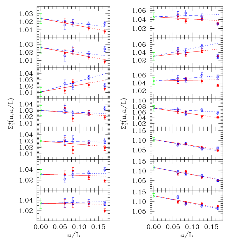
Figure C.1: Continuum extrapolations of $\Sigma_{\rm\scriptscriptstyle VA+AV;1}^{+}$ at fixed renormalized coupling $u$ for the improved action (full symbols, solid line) and the unimproved action (open symbols, dashed line). The $L/a=6$ data points have not been included in the fits. The value of $u$ increases from top to bottom and from left to right.

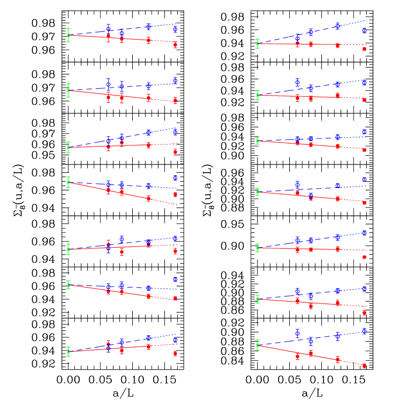
Figure C.2: Continuum extrapolations of $\Sigma_{\rm\scriptscriptstyle VA+AV;8}^{-}$ at fixed renormalized coupling $u$ for the improved action (full symbols, solid line) and the unimproved action (open symbols, dashed line). The $L/a=6$ data points have not been included in the fits. The value of $u$ increases from top to bottom and from left to right.

$~{}u$	$~{}\sigma^{+}_{1}(u)$	$~{}\sigma^{+}_{2}(u)$	$~{}\sigma^{+}_{3}(u)$	$~{}\sigma^{+}_{4}(u)$	$~{}\sigma^{+}_{5}(u)$
0.8873	1.024(6)	1.022(7)	1.026(7)	1.020(7)	1.020(7)
0.9944	1.026(7)	1.028(8)	1.029(7)	1.025(8)	1.025(8)
1.0989	1.011(7)	1.008(8)	1.012(7)	1.006(7)	1.007(7)
1.2430	1.030(8)	1.031(9)	1.034(8)	1.028(9)	1.028(8)
1.3293	1.030(8)	1.031(10)	1.034(9)	1.027(9)	1.027(9)
1.4300	1.031(9)	1.035(11)	1.035(9)	1.031(10)	1.031(10)
1.5553	1.034(10)	1.038(12)	1.040(10)	1.032(11)	1.033(11)
1.6950	1.046(9)	1.052(11)	1.055(10)	1.043(10)	1.044(10)
1.8811	1.030(10)	1.035(12)	1.039(10)	1.027(11)	1.028(11)
2.1000	1.045(9)	1.060(12)	1.058(10)	1.048(10)	1.050(10)
2.4484	1.074(10)	1.093(13)	1.095(11)	1.073(12)	1.074(12)
2.770	1.104(11)	1.143(15)	1.138(12)	1.110(13)	1.112(12)
3.111	1.118(12)	1.157(17)	1.157(14)	1.120(14)	1.124(14)
3.480	1.130(12)	1.186(18)	1.180(15)	1.140(15)	1.146(14)

$~{}u$	$~{}\sigma^{+}_{6}(u)$	$~{}\sigma^{+}_{7}(u)$	$~{}\sigma^{+}_{8}(u)$	$~{}\sigma^{+}_{9}(u)$
0.8873	1.018(7)	1.023(6)	1.017(7)	1.017(7)
0.9944	1.022(8)	1.025(7)	1.021(8)	1.021(8)
1.0989	1.005(7)	1.010(7)	1.004(7)	1.004(7)
1.2430	1.024(8)	1.029(8)	1.023(8)	1.024(8)
1.3293	1.024(9)	1.029(8)	1.023(9)	1.022(8)
1.4300	1.025(9)	1.029(8)	1.025(9)	1.024(9)
1.5553	1.027(10)	1.033(9)	1.025(10)	1.026(10)
1.6950	1.035(10)	1.044(9)	1.031(10)	1.033(9)
1.8811	1.018(10)	1.028(9)	1.016(10)	1.017(10)
2.1000	1.034(9)	1.041(9)	1.031(9)	1.033(9)
2.4484	1.050(11)	1.066(9)	1.045(10)	1.047(10)
2.770	1.072(11)	1.090(10)	1.063(11)	1.065(10)
3.111	1.073(12)	1.100(11)	1.064(11)	1.068(11)
3.480	1.084(12)	1.111(11)	1.074(12)	1.079(11)

Table C.5: Continuum extrapolations of $\Sigma_{\rm\scriptscriptstyle VA+AV;s}^{+}$ combining Clover and (perturbatively $\mbox{O}(a)$ improved) Wilson data. Linear dependence on $(a/L)$ is assumed for both actions. The $L/a=6$ data have not been taken into account.

$~{}u$	$~{}\sigma^{-}_{1}(u)$	$~{}\sigma^{-}_{2}(u)$	$~{}\sigma^{-}_{3}(u)$	$~{}\sigma^{-}_{4}(u)$	$~{}\sigma^{-}_{5}(u)$
0.8873	0.981(5)	0.978(6)	0.985(6)	0.973(5)	0.974(6)
0.9944	0.971(6)	0.975(7)	0.976(7)	0.971(6)	0.970(6)
1.0989	0.968(5)	0.963(7)	0.972(7)	0.959(6)	0.961(6)
1.2430	0.976(6)	0.980(8)	0.984(7)	0.974(6)	0.975(7)
1.3293	0.961(6)	0.960(9)	0.967(8)	0.955(7)	0.955(8)
1.4300	0.963(6)	0.975(8)	0.972(8)	0.968(7)	0.969(8)
1.5553	0.950(8)	0.952(11)	0.960(10)	0.944(8)	0.944(9)
1.6950	0.954(7)	0.962(10)	0.970(9)	0.949(8)	0.951(9)
1.8811	0.953(7)	0.956(11)	0.966(9)	0.943(9)	0.942(10)
2.1000	0.934(7)	0.967(11)	0.959(8)	0.947(8)	0.951(9)
2.4484	0.943(8)	0.971(13)	0.982(10)	0.941(10)	0.942(10)
2.770	0.911(8)	0.986(14)	0.974(10)	0.934(10)	0.938(11)
3.111	0.908(8)	0.987(15)	0.982(11)	0.930(11)	0.939(12)
3.480	0.896(10)	0.995(16)	0.983(12)	0.926(12)	0.935(13)

$~{}u$	$~{}\sigma^{-}_{6}(u)$	$~{}\sigma^{-}_{7}(u)$	$~{}\sigma^{-}_{8}(u)$	$~{}\sigma^{-}_{9}(u)$
0.8873	0.974(5)	0.982(6)	0.971(5)	0.971(5)
0.9944	0.971(6)	0.973(6)	0.968(5)	0.967(6)
1.0989	0.960(5)	0.970(6)	0.957(5)	0.958(6)
1.2430	0.973(6)	0.980(6)	0.969(6)	0.970(6)
1.3293	0.954(7)	0.963(7)	0.951(6)	0.950(7)
1.4300	0.967(7)	0.967(7)	0.962(6)	0.963(7)
1.5553	0.943(9)	0.953(8)	0.938(7)	0.938(8)
1.6950	0.947(8)	0.960(7)	0.939(7)	0.940(8)
1.8811	0.940(9)	0.956(8)	0.932(8)	0.932(9)
2.1000	0.944(8)	0.944(7)	0.931(7)	0.935(8)
2.4484	0.933(10)	0.956(8)	0.916(8)	0.917(9)
2.770	0.925(10)	0.932(8)	0.895(9)	0.898(10)
3.111	0.917(11)	0.935(9)	0.885(9)	0.893(10)
3.480	0.910(12)	0.927(10)	0.872(11)	0.880(12)

Table C.6: Continuum extrapolations of $\Sigma_{\rm\scriptscriptstyle VA+AV;s}^{-}$ combining Clover and (perturbatively $\mbox{O}(a)$ improved) Wilson data. Linear dependence on $(a/L)$ is assumed for both actions. The $L/a=6$ data have not been taken into account.

$s$	Fit	$s_{1}$	$s_{2}$		$s_{3}$	$s_{4}$		$\frac{\chi^{2}}{{\rm d.o.f.}}$	$\hat{Z}_{\rm s}^{+}(\mu_{\rm min})$
1	A	0.01755762	0.	00529(56)				1.27	1.095(16)
	B	0.01755762	0.	0006(23)	0.00167(81)			1.02	1.108(18)
	C	0.01755762	0.	00137(2)	0.00142(19)			0.95	1.105(15)
	D	0.01755762	$-$0.	0021(70)	0.0041(59)	$-$0.	0005(12)	1.10	1.111(19)
	E	0.01755762	0.	00137(2)	0.0012(12)	0.	00006(38)	1.03	1.106(16)
2	A	0.01755762	0.	00873(76)				1.75	1.050(21)
	B	0.01755762	$-$0.	0006(29)	0.0035(11)			0.99	1.067(22)
	C	0.01755762	$-$0.	00320(2)	0.00438(27)			0.97	1.076(20)
	D	0.01755762	$-$0.	0068(87)	0.0091(75)	$-$0.	0011(15)	1.02	1.074(24)
	E	0.01755762	$-$0.	00320(2)	0.0060(16)	$-$0.	00055(51)	0.95	1.069(21)
3	A	0.01755762	0.	00884(63)				1.83	0.990(17)
	B	0.01755762	0.	0014(25)	0.00275(90)			1.22	1.004(18)
	C	0.01755762	0.	00218(2)	0.00248(23)			1.13	1.001(15)
	D	0.01755762	$-$0.	0030(76)	0.0066(65)	$-$0.	0008(13)	1.29	1.008(19)
	E	0.01755762	0.	00218(2)	0.0024(13)	0.	00004(43)	1.22	1.001(16)
4	A	0.01755762	0.	00537(66)				1.57	1.163(20)
	B	0.01755762	$-$0.	0023(26)	0.00281(94)			0.95	1.182(22)
	C	0.01755762	$-$0.	00451(2)	0.00356(23)			0.93	1.191(19)
	D	0.01755762	$-$0.	0086(80)	0.0084(68)	$-$0.	0011(14)	0.97	1.190(24)
	E	0.01755762	$-$0.	00451(2)	0.0050(14)	$-$0.	00047(45)	0.91	1.183(20)
5	A	0.01755762	0.	00584(63)				1.60	1.143(19)
	B	0.01755762	$-$0.	0020(26)	0.00285(91)			0.92	1.164(21)
	C	0.01755762	$-$0.	00404(1)	0.00353(22)			0.89	1.173(18)
	D	0.01755762	$-$0.	0084(78)	0.0085(66)	$-$0.	0011(13)	0.93	1.171(23)
	E	0.01755762	$-$0.	00404(1)	0.0049(13)	$-$0.	00044(43)	0.88	1.165(19)

Table C.7: Fits to the continuum step scaling functions $\sigma_{\rm\scriptscriptstyle VA+AV;s}^{+}$ and results for the ratio $\hat{Z}_{\rm VA+AV;s}^{+}(\mu_{\rm min})$.

$s$	Fit	$s_{1}$	$s_{2}$		$s_{3}$	$s_{4}$		$\frac{\chi^{2}}{{\rm d.o.f.}}$	$\hat{Z}_{\rm s}^{+}(\mu_{\rm min})$
6	A	0.01755762	0.	00136(56)				0.96	1.294(20)
	B	0.01755762	$-$0.	0030(24)	0.00154(83)			0.75	1.309(22)
	C	0.01755762	$-$0.	00442(2)	0.00203(19)			0.72	1.317(18)
	D	0.01755762	$-$0.	0071(74)	0.0052(62)	$-$0.	0007(12)	0.79	1.315(24)
	E	0.01755762	$-$0.	00442(2)	0.0030(12)	$-$0.	00030(39)	0.74	1.310(20)
7	A	0.01755762	0.	00387(51)				1.06	1.138(16)
	B	0.01755762	0.	0004(22)	0.00122(77)			0.93	1.148(17)
	C	0.01755762	0.	00137(2)	0.00091(18)			0.87	1.144(14)
	D	0.01755762	$-$0.	0019(68)	0.0033(56)	$-$0.	0004(11)	1.00	1.151(19)
	E	0.01755762	0.	00137(2)	0.0006(11)	0.	00010(36)	0.94	1.146(16)
8	A	0.01755762	0.	00049(55)				0.87	1.338(20)
	B	0.01755762	$-$0.	0037(24)	0.00147(83)			0.67	1.353(22)
	C	0.01755762	$-$0.	00533(1)	0.00204(19)			0.66	1.362(18)
	D	0.01755762	$-$0.	0070(73)	0.0044(61)	$-$0.	0006(12)	0.71	1.358(25)
	E	0.01755762	$-$0.	00533(1)	0.0030(12)	$-$0.	00032(39)	0.66	1.355(20)
9	A	0.01755762	0.	00092(52)				0.92	1.316(19)
	B	0.01755762	$-$0.	0033(23)	0.00150(79)			0.70	1.332(21)
	C	0.01755762	$-$0.	00485(2)	0.00200(18)			0.67	1.341(17)
	D	0.01755762	$-$0.	0075(71)	0.0050(59)	$-$0.	0007(11)	0.72	1.338(23)
	E	0.01755762	$-$0.	00485(2)	0.0029(12)	$-$0.	00030(37)	0.68	1.333(19)

Table C.7: (continued)

$s$	Fit	$s_{1}$	$s_{2}$		$s_{3}$		$s_{4}$		$\frac{\chi^{2}}{{\rm d.o.f.}}$	$\hat{Z}_{\rm s}^{-}(\mu_{\rm min})$
1	A	$-0.03511524$	0.	00252(42)					1.87	0.497(6)
	B	$-0.03511524$	0.	0085(18)	$-$0.	00217(63)			1.03	0.490(7)
	C	$-0.03511524$	0.	01531(2)	$-$0.	00448(15)			2.06	0.479(6)
	D	$-0.03511524$	0.	0154(54)	$-$0.	0082(46)	0.	00122(91)	0.96	0.486(7)
	E	$-0.03511524$	0.	01531(2)	$-$0.	00815(92)	0.	00120(30)	0.88	0.486(6)
2	A	$-0.03511524$	0.	00941(69)					0.72	0.449(9)
	B	$-0.03511524$	0.	0069(26)	0.	00094(93)			0.70	0.450(9)
	C	$-0.03511524$	0.	00539(1)	0.	00146(25)			0.67	0.453(8)
	D	$-0.03511524$	0.	0049(77)	0.	0028(67)	$-$0.	0004(14)	0.76	0.451(10)
	E	$-0.03511524$	0.	00539(1)	0.	0023(14)	$-$0.	00029(46)	0.69	0.451(9)
3	A	$-0.03511524$	0.	00934(53)					0.75	0.401(6)
	B	$-0.03511524$	0.	0113(22)	$-$0.	00071(78)			0.75	0.399(6)
	C	$-0.03511524$	0.	01612(2)	$-$0.	00235(19)			1.05	0.392(5)
	D	$-0.03511524$	0.	0140(68)	$-$0.	0030(57)	0.	0005(11)	0.80	0.398(7)
	E	$-0.03511524$	0.	01612(2)	$-$0.	0048(11)	0.	00080(37)	0.74	0.397(6)
4	A	$-0.03511524$	0.	00407(52)					0.81	0.541(8)
	B	$-0.03511524$	0.	0042(20)	$-$0.	00006(73)			0.87	0.541(9)
	C	$-0.03511524$	0.	00276(2)	0.	00045(18)			0.85	0.544(8)
	D	$-0.03511524$	0.	0046(61)	$-$0.	0004(52)	0.	0001(11)	0.95	0.541(9)
	E	$-0.03511524$	0.	00276(2)	0.	0012(11)	$-$0.	00023(35)	0.88	0.542(8)
5	A	$-0.03511524$	0.	00466(56)					0.69	0.521(9)
	B	$-0.03511524$	0.	0041(23)	0.	00022(80)			0.74	0.522(9)
	C	$-0.03511524$	0.	00451(1)	0.	00007(20)			0.69	0.521(8)
	D	$-0.03511524$	0.	0044(67)	$-$0.	0001(57)	0.	0001(11)	0.81	0.522(10)
	E	$-0.03511524$	0.	00451(1)	$-$0.	0002(12)	0.	00008(39)	0.74	0.522(8)

Table C.8: Fits to the continuum step scaling functions $\sigma_{\rm\scriptscriptstyle VA+AV;s}^{-}$ and results for the ratio $\hat{Z}_{\rm VA+AV;s}^{-}(\mu_{\rm min})$.

$s$	Fit	$s_{1}$	$s_{2}$		$s_{3}$		$s_{4}$		$\frac{\chi^{2}}{{\rm d.o.f.}}$	$\hat{Z}_{\rm s}^{-}(\mu_{\rm min})$
6	A	$-0.03511524$	0.	00297(52)					0.81	0.551(9)
	B	$-0.03511524$	0.	0044(20)	$-$0.	00052(72)			0.83	0.550(9)
	C	$-0.03511524$	0.	00416(1)	$-$0.	00044(18)			0.77	0.550(8)
	D	$-0.03511524$	0.	0058(60)	$-$0.	0018(52)	0.	0003(10)	0.90	0.549(9)
	E	$-0.03511524$	0.	00416(1)	$-$0.	0004(11)	$-$0.	00001(35)	0.83	0.550(8)
7	A	$-0.03511524$	0.	00491(44)					1.34	0.462(6)
	B	$-0.03511524$	0.	0094(19)	$-$0.	00162(66)			0.95	0.457(6)
	C	$-0.03511524$	0.	01531(2)	$-$0.	00362(15)			1.62	0.447(5)
	D	$-0.03511524$	0.	0154(58)	$-$0.	0068(48)	0.	00103(95)	0.92	0.453(7)
	E	$-0.03511524$	0.	01531(2)	$-$0.	00673(95)	0.	00102(31)	0.85	0.453(6)
8	A	$-0.03511524$	$-$0.	00017(45)					1.00	0.622(9)
	B	$-0.03511524$	0.	0021(18)	$-$0.	00082(64)			0.95	0.620(9)
	C	$-0.03511524$	0.	00194(1)	$-$0.	00078(16)			0.88	0.621(8)
	D	$-0.03511524$	0.	0048(54)	$-$0.	0033(46)	0.	00051(94)	1.01	0.618(10)
	E	$-0.03511524$	0.	00194(1)	$-$0.	00089(95)	0.	00004(31)	0.95	0.621(8)
9	A	$-0.03511524$	0.	00038(50)					0.89	0.600(9)
	B	$-0.03511524$	0.	0022(20)	$-$0.	00065(72)			0.89	0.599(10)
	C	$-0.03511524$	0.	00370(2)	$-$0.	00118(18)			0.87	0.595(9)
	D	$-0.03511524$	0.	0057(61)	$-$0.	0038(52)	0.	0006(10)	0.94	0.596(10)
	E	$-0.03511524$	0.	00370(2)	$-$0.	0022(11)	0.	00032(35)	0.87	0.598(9)

Table C.8: (continued)

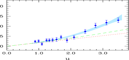
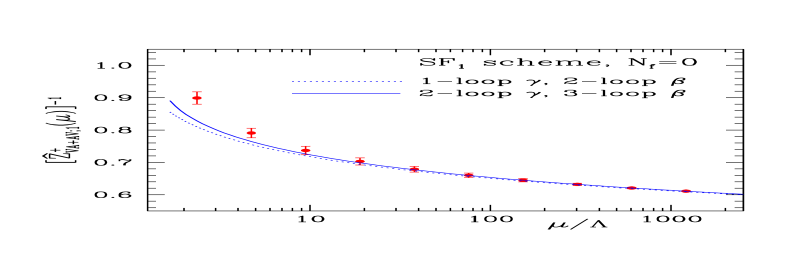
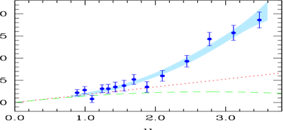
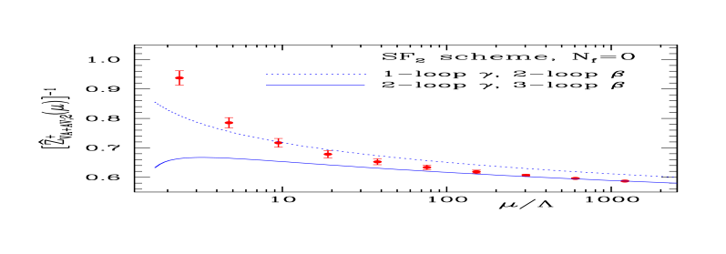
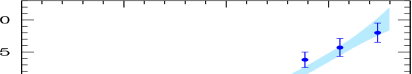
Figure C.3: Left column: The step scaling function $\sigma_{\rm\scriptscriptstyle VA+AV;s}^{+}(u)$ (discrete points) as obtained non-perturbatively from combined fits to Clover and Wilson data. The shaded area is the result of fit D to the points (see text). The dotted (dashed) line is the LO (NLO) perturbative result. Right column: RG running of $O_{\rm\scriptscriptstyle VA+AV}^{+}$ obtained non-perturbatively (discrete points) at specific values of the renormalization scale $\mu$, in units of $\Lambda$ (taken from ref. [4]). The lines are perturbative results at the indicated order for the Callan-Symanzik $\beta$-function and the operator anomalous dimension $\gamma$.

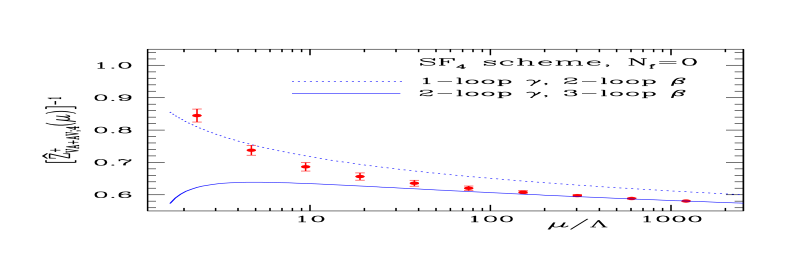
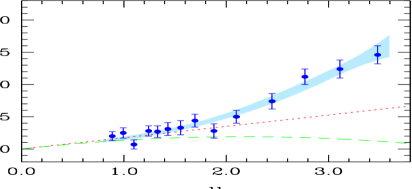
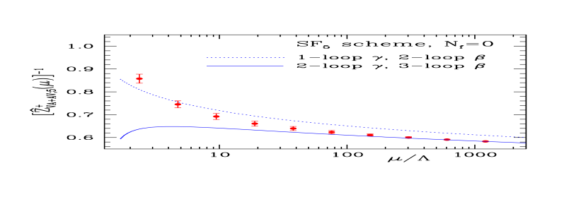
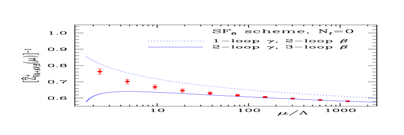
Figure C.3: (continued)

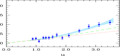
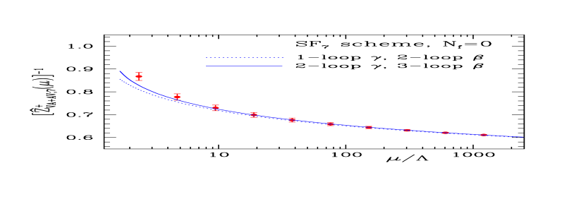
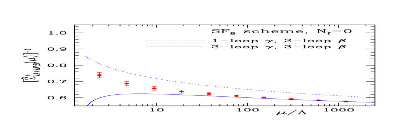
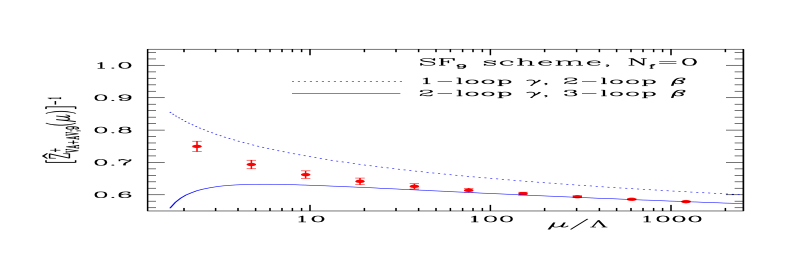
Figure C.3: (continued)

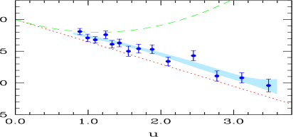
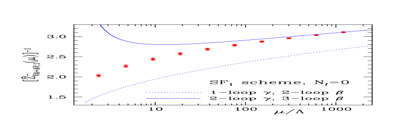
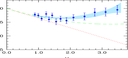
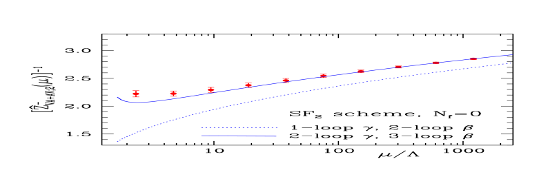
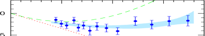
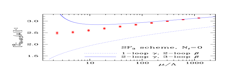
Figure C.4: Left column: The step scaling function $\sigma_{\rm\scriptscriptstyle VA+AV;s}^{-}(u)$ (discrete points) as obtained non-perturbatively from combined fits to Clover and Wilson data. The shaded area is the result of fit D to the points (see text). The dotted (dashed) line is the LO (NLO) perturbative result. Right column: RG running of $O_{\rm\scriptscriptstyle VA+AV}^{-}$ obtained non-perturbatively (discrete points) at specific values of the renormalization scale $\mu$, in units of $\Lambda$ (taken from ref. [4]). The lines are perturbative results at the indicated order for the Callan-Symanzik $\beta$-function and the operator anomalous dimension $\gamma$.

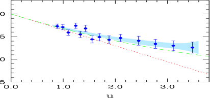
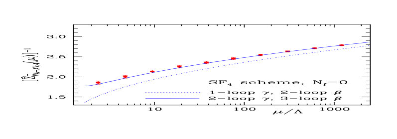
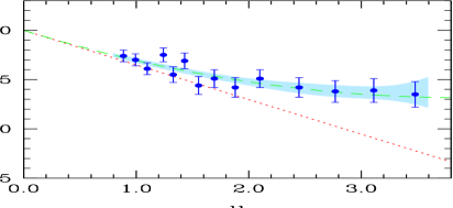
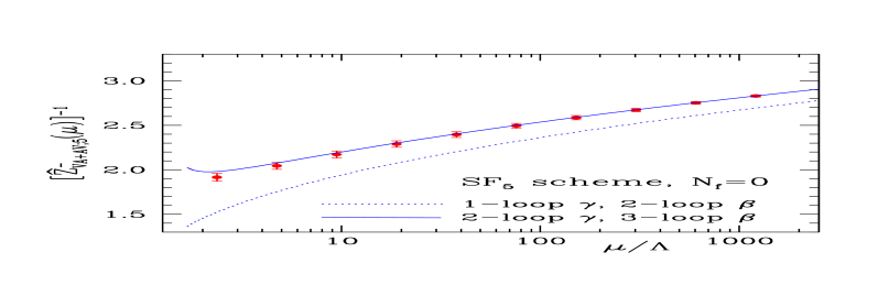
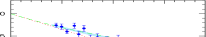
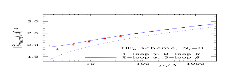
Figure C.4: (continued)

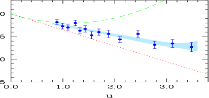
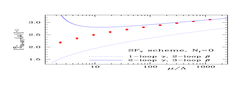
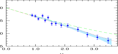
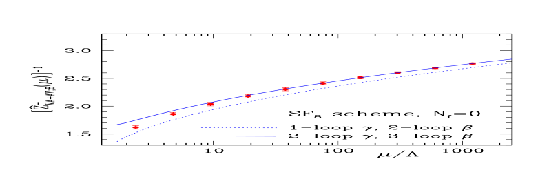
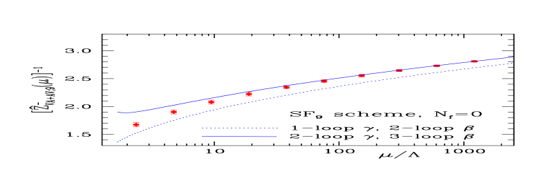
Figure C.4: (continued)

		Clover action		Wilson action
$\beta~{}~{}~{}$	$\frac{L}{a}$	$~{}~{}~{}~{}~{}~{}\kappa_{\rm cr}$	$Z_{\rm\scriptscriptstyle VA+AV;s}^{+}$	$~{}~{}~{}~{}~{}~{}\kappa_{\rm cr}$	$Z_{\rm\scriptscriptstyle VA+AV;s}^{+}$
6.0219	8	0.135043(17)	0.7985(27)	0.153371(10)	0.6435(28)
6.1628	10	0.135643(11)	0.8228(17)	0.152012(7)	0.6743(24)
6.2885	12	0.135739(13)	0.8400(20)	0.150752(10)	0.6978(33)
6.4956	16	0.135577(7)	0.8758(46)	0.148876(13)	0.7377(48)
6.0219	8	0.135043(17)	0.8661(42)	0.153371(10)	0.6802(37)
6.1628	10	0.135643(11)	0.8873(26)	0.152012(7)	0.7145(33)
6.2885	12	0.135739(13)	0.9029(31)	0.150752(10)	0.7413(46)
6.4956	16	0.135577(7)	0.9412(74)	0.148876(13)	0.7861(66)
6.0219	8	0.135043(17)	0.8851(36)	0.153371(10)	0.7010(33)
6.1628	10	0.135643(11)	0.9105(22)	0.152012(7)	0.7370(29)
6.2885	12	0.135739(13)	0.9272(26)	0.150752(10)	0.7647(40)
6.4956	16	0.135577(7)	0.9667(61)	0.148876(13)	0.8096(58)
6.0219	8	0.135043(17)	0.7911(32)	0.153371(10)	0.6232(29)
6.1628	10	0.135643(11)	0.8100(20)	0.152012(7)	0.6534(26)
6.2885	12	0.135739(13)	0.8252(24)	0.150752(10)	0.6768(36)
6.4956	16	0.135577(7)	0.8585(56)	0.148876(13)	0.7183(52)
6.0219	8	0.135043(17)	0.7963(32)	0.153371(10)	0.6226(29)
6.1628	10	0.135643(11)	0.8153(20)	0.152012(7)	0.6534(25)
6.2885	12	0.135739(13)	0.8307(24)	0.150752(10)	0.6770(35)
6.4956	16	0.135577(7)	0.8633(56)	0.148876(13)	0.7215(50)

Table C.9: Results for $Z_{\rm\scriptscriptstyle VA+AV;s}^{+}(g_{0},L/a)$ at fixed scale $L=1.436\,r_{0}$ (corresponding to $\mu_{\rm min}=(2L_{\rm max})^{-1}$). Each block contains the results from a different renormalization condition ($s=1,\ldots,5$).

		Clover action		Wilson action
$\beta~{}~{}~{}$	$\frac{L}{a}$	$~{}~{}~{}~{}~{}~{}\kappa_{\rm cr}$	$Z_{\rm\scriptscriptstyle VA+AV;s}^{+}$	$~{}~{}~{}~{}~{}~{}\kappa_{\rm cr}$	$Z_{\rm\scriptscriptstyle VA+AV;s}^{+}$
6.0219	8	0.135043(17)	0.7058(25)	0.153371(10)	0.5670(25)
6.1628	10	0.135643(11)	0.7236(16)	0.152012(7)	0.5919(22)
6.2885	12	0.135739(13)	0.7388(19)	0.150752(10)	0.6104(29)
6.4956	16	0.135577(7)	0.7686(43)	0.148876(13)	0.6486(42)
6.0219	8	0.135043(17)	0.7722(24)	0.153371(10)	0.6209(26)
6.1628	10	0.135643(11)	0.7948(15)	0.152012(7)	0.6501(22)
6.2885	12	0.135739(13)	0.8111(18)	0.150752(10)	0.6719(29)
6.4956	16	0.135577(7)	0.8446(40)	0.148876(13)	0.7122(42)
6.0219	8	0.135043(17)	0.6902(24)	0.153371(10)	0.5520(23)
6.1628	10	0.135643(11)	0.7071(15)	0.152012(7)	0.5764(20)
6.2885	12	0.135739(13)	0.7219(17)	0.150752(10)	0.5946(27)
6.4956	16	0.135577(7)	0.7501(40)	0.148876(13)	0.6319(40)
6.0219	8	0.135043(17)	0.6947(23)	0.153371(10)	0.5515(22)
6.1628	10	0.135643(11)	0.7117(14)	0.152012(7)	0.5764(19)
6.2885	12	0.135739(13)	0.7267(17)	0.150752(10)	0.5948(26)
6.4956	16	0.135577(7)	0.7543(39)	0.148876(13)	0.6347(37)

Table C.10: Results for $Z_{\rm\scriptscriptstyle VA+AV;s}^{+}(g_{0},L/a)$ at fixed scale $L=1.436\,r_{0}$ (corresponding to $\mu_{\rm min}=(2L_{\rm max})^{-1}$). Each block contains the results from a different renormalization condition ($s=6,\ldots,9$).

		Clover action		Wilson action
$\beta~{}~{}~{}$	$\frac{L}{a}$	$~{}~{}~{}~{}~{}~{}\kappa_{\rm cr}$	$Z_{\rm\scriptscriptstyle VA+AV;s}^{-}$	$~{}~{}~{}~{}~{}~{}\kappa_{\rm cr}$	$Z_{\rm\scriptscriptstyle VA+AV;s}^{-}$
6.0219	8	0.135043(17)	0.5499(18)	0.153371(10)	0.6368(27)
6.1628	10	0.135643(11)	0.5561(11)	0.152012(7)	0.6212(21)
6.2885	12	0.135739(13)	0.5573(13)	0.150752(10)	0.6115(29)
6.4956	16	0.135577(7)	0.5592(30)	0.148876(13)	0.6006(40)
6.0219	8	0.135043(17)	0.6474(36)	0.153371(10)	0.7150(40)
6.1628	10	0.135643(11)	0.6472(21)	0.152012(7)	0.7023(32)
6.2885	12	0.135739(13)	0.6452(25)	0.150752(10)	0.6922(44)
6.4956	16	0.135577(7)	0.6524(57)	0.148876(13)	0.6895(67)
6.0219	8	0.135043(17)	0.6743(25)	0.153371(10)	0.7719(35)
6.1628	10	0.135643(11)	0.6814(16)	0.152012(7)	0.7570(28)
6.2885	12	0.135739(13)	0.6809(18)	0.150752(10)	0.7497(38)
6.4956	16	0.135577(7)	0.6866(41)	0.148876(13)	0.7311(51)
6.0219	8	0.135043(17)	0.5549(24)	0.153371(10)	0.6056(26)
6.1628	10	0.135643(11)	0.5538(14)	0.152012(7)	0.5944(21)
6.2885	12	0.135739(13)	0.5529(17)	0.150752(10)	0.5854(29)
6.4956	16	0.135577(7)	0.5558(37)	0.148876(13)	0.5869(46)
6.0219	8	0.135043(17)	0.5516(26)	0.153371(10)	0.6057(29)
6.1628	10	0.135643(11)	0.5514(15)	0.152012(7)	0.5941(23)
6.2885	12	0.135739(13)	0.5520(18)	0.150752(10)	0.5858(32)
6.4956	16	0.135577(7)	0.5562(40)	0.148876(13)	0.5868(50)

Table C.11: Results for $Z_{\rm\scriptscriptstyle VA+AV;s}^{-}(g_{0},L/a)$ at fixed scale $L=1.436\,r_{0}$ (corresponding to $\mu_{\rm min}=(2L_{\rm max})^{-1}$). Each block contains the results from a different renormalization condition ($s=1,\ldots,5$).

		Clover action		Wilson action
$\beta~{}~{}~{}$	$\frac{L}{a}$	$~{}~{}~{}~{}~{}~{}\kappa_{\rm cr}$	$Z_{\rm\scriptscriptstyle VA+AV;s}^{-}$	$~{}~{}~{}~{}~{}~{}\kappa_{\rm cr}$	$Z_{\rm\scriptscriptstyle VA+AV;s}^{-}$
6.0219	8	0.135043(17)	0.5276(23)	0.153371(10)	0.5960(27)
6.1628	10	0.135643(11)	0.5278(14)	0.152012(7)	0.5819(22)
6.2885	12	0.135739(13)	0.5279(16)	0.150752(10)	0.5700(29)
6.4956	16	0.135577(7)	0.5328(36)	0.148876(13)	0.5689(44)
6.0219	8	0.135043(17)	0.5883(19)	0.153371(10)	0.6837(30)
6.1628	10	0.135643(11)	0.5948(12)	0.152012(7)	0.6677(23)
6.2885	12	0.135739(13)	0.5956(14)	0.150752(10)	0.6586(32)
6.4956	16	0.135577(7)	0.5999(32)	0.148876(13)	0.6432(41)
6.0219	8	0.135043(17)	0.4841(20)	0.153371(10)	0.5364(22)
6.1628	10	0.135643(11)	0.4835(12)	0.152012(7)	0.5243(17)
6.2885	12	0.135739(13)	0.4837(14)	0.150752(10)	0.5143(24)
6.4956	16	0.135577(7)	0.4856(30)	0.148876(13)	0.5163(38)
6.0219	8	0.135043(17)	0.4812(21)	0.153371(10)	0.5365(23)
6.1628	10	0.135643(11)	0.4813(12)	0.152012(7)	0.5241(18)
6.2885	12	0.135739(13)	0.4829(14)	0.150752(10)	0.5147(26)
6.4956	16	0.135577(7)	0.4860(31)	0.148876(13)	0.5162(40)

Table C.12: Results for $Z_{\rm\scriptscriptstyle VA+AV;s}^{-}(g_{0},L/a)$ at fixed scale $L=1.436\,r_{0}$ (corresponding to $\mu_{\rm min}=(2L_{\rm max})^{-1}$). Each block contains the results from a different renormalization condition ($s=6,\ldots,9$).

References

- [1] G. Martinelli, C. Pittori, C. T. Sachrajda, M. Testa and A. Vladikas, Nucl. Phys. B445 (1995) 81.
- [2] K. Jansen et al., Phys. Lett. B372 (1996) 275.
- [3] M. Lüscher, R. Sommer, P. Weisz and U. Wolff, Nucl. Phys. B413 (1994) 481.
- [4] Alpha Collab., S. Capitani et al., Nucl. Phys. B544 (1999) 669.
- [5] Alpha Collab., M. Guagnelli et al., JHEP 0405 (2004) 001.
-
[6]
Alpha Collab., A. Bode et al., Phys. Lett. B 515 (2001) 49;
Alpha Collab., F. Knechtli et al., Nucl. Phys. Proc. Suppl. 119 (2003) 320;
Alpha Collab., M. Della Morte et al., Nucl. Phys. Proc. Suppl. 119 (2003) 439;
Alpha Collab., F. Knechtli et al., Nucl. Phys. Proc. Suppl. 129 (2004) 814. -
[7]
M. Guagnelli, K. Jansen and R. Petronzio, Phys. Lett. B457 (1999) 153;
ZeRo Collab., M. Guagnelli et al., Nucl. Phys. B 664 (2003) 276;
ZeRo Collab., A. Shindler et al., Nucl. Phys. Proc. Suppl. 129 (2004) 278;
I. Wetzorke, K. Jansen, F. Palombi and A. Shindler, Nucl. Phys. Proc. Suppl. 140 (2005) 393. - [8] Alpha Collab., J. Heitger, M. Kurth and R. Sommer, Nucl. Phys. B669 (2003) 173.
- [9] C. W. Bernard, T. Draper, G. Hockney and A. Soni, Nucl. Phys. Proc. Suppl. 4 (1988) 483.
- [10] A. Donini, V. Giménez, G. Martinelli, M. Talevi and A. Vladikas, Eur. Phys. J. C10 (1999) 121.
- [11] R. Frezzotti, P. A. Grassi, S. Sint and P. Weisz, JHEP 0108 (2001) 058.
- [12] B. Sheikholeslami and R. Wohlert, Nucl. Phys. B259 (1985) 572.
- [13] Alpha Collab., M. Guagnelli et al., Nucl. Phys. Proc. Suppl. 106 (2002) 320; ibid. 119 (2003) 436.
- [14] Alpha Collab., F. Palombi, C. Pena and S. Sint, Nucl. Phys. Proc. Suppl. 140 (2005) 362; Alpha Collab., F. Palombi, C. Pena and S. Sint, “A perturbative study of two four-quark operators in finite volume renormalization schemes”, Preprint DESY 05-070, CERN-PH-TH/2005-45, FTUAM-05-2, IFT-UAM-CSIC/05-16, e-Print Archive: hep-lat/0505003.
- [15] Alpha Collab., S. Sint and P. Weisz, Nucl. Phys. B545 (1999) 529.
- [16] S. Weinberg, Phys. Rev. D8 (1973) 3497.
-
[17]
G.C. Rossi and M. Testa, Nucl. Phys. B163 (1980) 109; ibid. B176
(1980) 477; ibid. B237 (1984) 442;
K. Symanzik, Nucl. Phys. B190[FS3] (1981) 1;
M. Lüscher, Nucl. Phys. B254 (1985) 52;
G.C. Rossi and K. Yoshida, Nuovo Cim. 11D (1989) 101;
J.P. Leroy, J. Micheli, G.C. Rossi and K. Yoshida, Z. Phys. C48 (1990) 653. - [18] M. Lüscher, R. Narayanan, P. Weisz and U. Wolff, Nucl. Phys. B384 (1992) 168.
- [19] S. Sint, Nucl. Phys. B421 (1994) 135; ibid. B451 (1995) 416.
- [20] M. Lüscher, S. Sint, R. Sommer and P. Weisz, Nucl. Phys. B478 (1996) 365.
- [21] M. Lüscher and P. Weisz, Nucl. Phys. B479 (1996) 429.
- [22] M. Lüscher, S. Sint, R. Sommer and H. Wittig, Nucl. Phys. B491 (1997) 344.
- [23] Alpha Collab., M. Guagnelli, R. Sommer and H. Wittig, Nucl. Phys. B535 (1998) 389.
- [24] S. Necco and R. Sommer, Nucl. Phys. B622 (2002) 328.
- [25] R. Frezzotti and G. C. Rossi, JHEP 0408 (2004) 007.
-
[26]
M. Lüscher et al., Nucl. Phys. B491 (1997) 323;
R.G. Edwards, U.M. Heller and T.R. Klassen, Nucl. Phys. Proc. Suppl. 63 (1998) 847. - [27] Alpha Collab., A. Bode, P. Weisz and U. Wolff, Nucl. Phys. B540 (1999) 491.
- [28] Alpha Collab., G. de Divitiis et al., Nucl. Phys. B437 (1995) 447.
- [29] Alpha Collab., M. Guagnelli, J. Heitger, C. Pena and A. Vladikas, Nucl. Phys. Proc. Suppl. 129 (2004) 402.
- [30] Y. Taniguchi, “Schrödinger Functional Formalism with Ginsparg-Wilson Fermion”, Preprint UTHEP-501, UTCCS-P-11, e-Print Archive: hep-lat/0412024.
- [31] P. Hernández, K. Jansen, L. Lellouch and H. Wittig, JHEP 0107 (2001) 018.
- [32] Alpha Collab., P. Dimopoulos et al. Nucl. Phys. Proc. Suppl. 129 (2004) 308; ibid. 140 (2005) 362.