Low-lying mode contribution to the quenched meson correlators in the $\epsilon$-regime

Abstract

We present a quenched calculation of meson correlators with the overlap fermion at very small masses 2.6–13 MeV. In this region the pion Compton wavelength is larger than our lattice size ($L\simeq$ 1.23 fm) and the system is in the so-called $\epsilon$-regime of chiral perturbation theory. We found that the scalar and pseudo-scalar correlators are precisely approximated by a few hundred low-lying fermion eigenmodes in this regime, whereas axial-vector correlator receives significant contributions from higher eigenmodes. We also measure the disconnected pseudo-scalar correlator, which is well saturated with the low-lying modes. Matching these lattice data with the one-loop expressions for the correlators in quenched chiral perturbation theory, we evaluate the decay constant $F_{\pi}$ and the chiral condensate $\Sigma$ as well as the parameters $m_{0}^{2}$ and $\alpha$, which describe the artifacts of the quenched approximation.

1 Introduction

Chiral perturbation theory (ChPT) provides a systematic method to calculate low energy dynamics of QCD, though it contains unknown parameters at each order of the expansion in pion mass squared $m_{\pi}^{2}$ and momentum squared $p_{\pi}^{2}$. At the lowest order these parameters are the pion decay constant $F_{\pi}$ and the chiral condensate $\Sigma$, and there are 10 other low energy constants in the next-to-leading order [1]. It is one of the important tasks of lattice QCD to calculate these low energy constants non-perturbatively from the first principles. In the standard approach, however, this is very demanding because one has to work on large enough lattices satisfying $m_{\pi}L\gg 1$ to avoid possible finite size effects. Taking the chiral limit $m_{\pi}\to 0$ and the continuum limit while satisfying this condition will be prohibitively time consuming even with today’s fastest supercomputers, especially when the quarks are treated dynamically.

In the so-called $\epsilon$-regime [2, 3, 4], where the linear extent of the space-time box is smaller than the pion Compton wave length $L\ll 1/m_{\pi}$ (but larger than the QCD scale $1/\Lambda_{\mathrm{QCD}}\ll L$, which assures that the pion can be treated as a point particle and other heavier hadrons are decoupled. ), the chiral Lagrangian is still applicable except that the expansion parameter is given by $\epsilon^{2}\sim m_{\pi}/\Lambda\sim p_{\pi}^{2}/\Lambda^{2}$, where $\Lambda$ is a cutoff scale of the chiral Lagrangian roughly around 1 GeV. An important observation is that the low energy constants in the chiral Lagrangian are defined at the cutoff scale commonly for both the standard and $\epsilon$-regimes. Therefore, one can determine the low energy constants in the $\epsilon$-regime and use them in the standard ChPT. In this way one can avoid the problem of the chiral limit while keeping the large lattice volume. Analytic calculation of meson correlation functions in the $\epsilon$-regime is available for both quenched and unquenched theories [5, 6, 7].

In the study of the chiral regime of lattice QCD the chiral symmetry plays an essential role. First of all, one must treat pions near the massless limit, which appear as a result of the spontaneous chiral symmetry breaking. Furthermore, it is known that the effects of fermion zero modes become important in the $\epsilon$-regime [8] and the correlators depend strongly on the topological charge of the background gauge field [5, 6]. The lattice fermion formulations preserving chiral symmetry [9] (by satisfying the Ginsparg-Wilson relation [10]) is now commonly used (but only in the quenched approximation). In this work we use the Neuberger’s overlap-Dirac operator [11, 12]. With this formulation there is no fundamental problem to approach the chiral limit as required in the study of the $\epsilon$-regime, but the computational cost to invert the overlap-Dirac operator increases for small quark masses.

In the chiral regime the meson correlators are largely affected by the low-lying fermion modes especially by the chiral zero modes. In this work we explicitly study the effects of such low-lying modes using the eigenmode decomposition of the fermion propagator. In the quenched approximation we find that the connected scalar and pseudo-scalar meson correlators are reproduced to 98–99.9% accuracy (depending on channels) with only 200 lowest-lying eigenmodes on a $10^{3}\times 20$ at small quark masses (2.6 MeV $\lesssim m\lesssim$ 13 MeV). Such saturation was previously found in Refs. DeGrand:2000gq,DeGrand:2003sf, but it should be better in the $\epsilon$-regime (In our study, $L$ satisfies $m_{\pi}L\sim 0.6$ and $\Lambda_{QCD}L\sim 3$.). An advantage of such eigenmode decomposition is that the meson correlators can be averaged over space-time points without much extra computational costs. The statistical fluctuations originating from the local bumps of zero-mode wave function are suppressed by the space-time averaging and thus we can avoid the large noise as found in Ref. Bietenholz:2003bj. The low-mode averaging was also used in recent studies [16, 17].

Matching our numerical data of the axial-vector, scalar and pseudo-scalar correlators with the quenched ChPT (QChPT) expressions, we extract the leading order low-energy constants $\Sigma$ and $F_{\pi}$ as well as the parameters appearing due to the quenched artifact, $\alpha$ and $m_{0}$. The axial-vector correlator is most sensitive to $F_{\pi}$ while $\Sigma$ is precisely determined by the connected scalar and pseudo-scalar correlators. We also investigate the chiral condensates and the disconnected (hairpin) correlators for the pseudo-scalar channel. In general we find good agreement between the lattice data and the QChPT predictions for topological charge $|Q|$ = 0 and 1 sectors, but the larger topological sectors deviate significantly, which may suggest breakdown of the $\epsilon$-expansion in the QChPT at large $|Q|$.

The axial-vector correlator has already been calculated in the recent works [15, 17]. Bietenholz et al. [15] worked at a relatively larger quark mass ($\sim$ 21 MeV) and found that the correlator is well fitted with the QChPT formula for a large enough lattice size ($L>$ 1.1 fm). They also pointed out that the signal is very noisy at $|Q|$ = 0. Using the low-mode averaging technique [16, 17], Giusti et al. pushed the quark mass down to 10 MeV and found an encouraging agreement of $F_{\pi}$ measured in the $\epsilon$-regime as that from the standard measurement. Their result is $F_{\pi}$ = 102(4) MeV in the $\epsilon$-regime. There is another interesting work by the same authors [18], who investigated the divergent (as $\sim 1/m^{2}$) contributions of zero mode in the massless limit and matched them with the theoretical expectations from QChPT.

This paper is organized as follows. In Section 2, we review the quenched chiral perturbation theory (QChPT) in the $\epsilon$-regime following the discussions of Damgaard et al. [5]. We describe the details of our simulation in Section 3 and study the low-lying eigenmode dominance in Section 4. In Section 5 we present our results for the chiral condensate and meson correlators and the comparison with the QChPT. Conclusions are given in Section 6.

2 Quenched chiral perturbation theory in the $\epsilon$-regime

In this section, we briefly review quenched chiral perturbation theory (QChPT) in the $\epsilon$-regime [5] and summarize the relevant formulae for our analysis of meson correlation functions.

The partition function of QChPT with $N_{v}$ valence quarks is written as

$$Z(\theta,M) = \int dU\exp\left(-\int d^{4}x\mathcal{L}^{\theta}_{M}(x)\right),$$ (1)

where the Lagrangian $\mathcal{L}^{\theta}_{M}$ is given by

$$\mathcal{L}^{\theta}_{M}(x) = \frac{F_{\pi}^{2}}{4}\mbox{Str}(\partial_{\mu}U(x)^{-1}\partial_{\mu}U(x))-\frac{m\Sigma}{2}\mbox{Str}(U_{\theta}U(x)+U(x)^{-1}U_{\theta}^{-1})$$ (2)

$$+\frac{m_{0}^{2}}{2N_{c}}\Phi(x)^{2}+\frac{\alpha}{2N_{c}}\partial_{\mu}\Phi(x)\partial_{\mu}\Phi(x)$$

at the leading order of $m_{\pi}^{2}$ and $p_{\pi}^{2}$ expansion. The field variable $U(x)$ is integrated over a sub-manifold of the super-group $Gl(N_{v}|N_{v})$, the maximally symmetric Riemannian sub-manifold, which is characterized by a matrix of form

$$U=\left(\begin{array}[]{cc}A&B\\ C&D\end{array}\right),\;\;\;\;\;A\in U(N_{v}),\;\;\;\;\;D\in Gl(N_{v})/U(N_{v}),$$ (3)

and Grassmannian $N_{v}\times N_{v}$ matrices $B$ and $C$. Str denotes the super-trace. The mass term corresponds to the choice of mass matrix $M=(mI_{v}+m\tilde{I_{v}})$ with $I_{v}$ and $\tilde{I_{v}}$ the identity matrix in the fermion-fermion and boson-boson blocks respectively. The effect of CP violating $\theta$ term enters through $U_{\theta}\equiv\exp(i\theta/N_{v})I_{N_{v}}+\tilde{I}_{N_{v}}$. In the quenched approximation the singlet field $\Phi(x)\equiv\frac{F_{\pi}}{\sqrt{2}}\mbox{Str}[-i\ln U(x)]$ does not decouple, and the couplings $m_{0}^{2}$ and $\alpha$ are introduced [19].

The $\epsilon$-regime [2, 3, 4] is realized when the quark mass is small enough that the pion Compton wavelength $\sim 1/m_{\pi}$ is larger than the linear extent of the space-time $L$. The systematic expansion is then reorganized and the expansion parameter is given by $\epsilon^{2}\sim m_{\pi}/4\pi F_{\pi}\sim 1/(LF_{\pi})^{2}$. Unlike the standard ChPT the zero mode of pion gives important contribution and one must explicitly integrate out the constant mode of $U(x)$. This is done by writing as

$$U(x)=U_{0}\exp i\frac{\sqrt{2}\xi(x)}{F_{\pi}}$$ (4)

and integrating over the constant mode $U_{0}$. One obtains the partition function at a fixed topological charge $Q$ by Fourier transforming (1).

$$Z_{Q}(M) \equiv \frac{1}{2\pi}\int_{-\pi}^{+\pi}\!d\theta e^{i\theta Q}Z(\theta,M)$$ (5)

$$= \frac{1}{\sqrt{2\pi\langle Q^{2}\rangle}}e^{-Q^{2}/2\langle Q^{2}\rangle}\int dU_{0}d\xi\,(\mathrm{S}\det U_{0})^{Q}\exp\left[\frac{m\Sigma V}{2}\mbox{Str}(U_{0}+U_{0}^{-1})\right.$$

$$+\left.\int\!d^{4}x\left(-\frac{1}{2}\mbox{Str}(\partial_{\mu}\xi\partial_{\mu}\xi)-\frac{m_{0}^{2}}{2N_{c}}(\mbox{Str}\xi)^{2}-\frac{\alpha}{2N_{c}}(\partial_{\mu}\mbox{Str}\xi)^{2}\right)+O(\epsilon^{4})\right],$$

where $dU_{0}$ denotes the Haar measure of the maximally Riemannian sub-manifold of $Gl(N_{v}|N_{v})$. The topological charge distributes as Gaussian with variance

$$\frac{\langle Q^{2}\rangle}{V}=\frac{F_{\pi}^{2}m_{0}^{2}}{2N_{c}}$$ (6)

in the quenched theory, which is an exact equation for $V\to\infty$. It shows a good contrast with the full theory, for which $\langle Q^{2}\rangle=m\Sigma V/N_{f}$ is expected for $N_{f}$ flavors.

We note that in the quenched approximation the Gaussian approximation of the Fourier transform in $\theta$ is justified only for small topological charge that satisfies $|Q|\ll\langle Q^{2}\rangle$. (See Appendix for the details.) Therefore, all the results shown below are valid only for small $|Q|$. We investigate how this breakdown of the effective theory occurs using the lattice data.

In the following we consider $N_{v}$ = 1 and 2 as we are interested in the system with two light quarks. All the results are obtained by the perturbation of $\xi$ fields and the exact integration over zero mode $U_{0}$, which can be written in terms of the Bessel functions.

At the tree-level the scalar condensate is given as

$$-\langle\bar{\psi}\psi\rangle_{Q}\equiv\Sigma_{Q}(\mu)=\Sigma\mu(I_{|Q|}(\mu)K_{|Q|}(\mu)+I_{|Q|+1}(\mu)K_{|Q|-1}(\mu))+\Sigma\frac{|Q|}{\mu}$$ (7)

with $\mu\equiv m\Sigma V$. $I_{|Q|}(\mu)$ and $K_{|Q|}(\mu)$ denote the modified Bessel functions. The $\mu$ dependence of $\Sigma_{Q}(\mu)$ is shown in Figure 1. Near the massless limit it asymptotically behaves as $\Sigma_{|Q|}(\mu)\to\Sigma|Q|/\mu$ for $|Q|>0$. One-loop correction does not change its functional form [20]

$$\Sigma^{\mathrm{1-loop}}_{Q}(\mu)=\Sigma_{\mathrm{eff}}\mu^{\prime}(I_{|Q|}(\mu^{\prime})K_{|Q|}(\mu^{\prime})+I_{|Q|+1}(\mu^{\prime})K_{|Q|-1}(\mu^{\prime}))+\Sigma_{\mathrm{eff}}\frac{|Q|}{\mu^{\prime}}=\Sigma_{Q}(\mu^{\prime}),$$ (8)

but the parameters $\mu$ and $\Sigma$ are shifted to $\mu^{\prime}$ and $\Sigma_{\mathrm{eff}}$:

$$\mu^{\prime} \equiv m\Sigma_{\mathrm{eff}}V,$$ (9)

$$\Sigma_{\mathrm{eff}} \equiv \Sigma\left(1+\frac{m_{0}^{2}\bar{G}(0)+\alpha\bar{\Delta}(0)}{N_{c}F_{\pi}^{2}}\right).$$ (10)

Here, parameters $\bar{G}(0)$ and $\bar{\Delta}(0)$ are ultraviolet divergent tadpole integrals,

$$\bar{G}(x) \equiv \frac{1}{V}\sum_{p\neq 0}\frac{e^{ipx}}{p^{4}},$$ (11)

$$\bar{\Delta}(x) \equiv \frac{1}{V}\sum_{p\neq 0}\frac{e^{ipx}}{p^{2}},$$ (12)

which need to be renormalized. In our analysis they are to be determined by matching with lattice data.

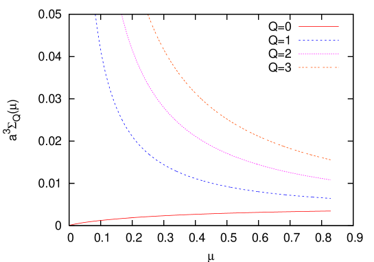
Figure 1: $\Sigma_{Q}(\mu)$ in different topological sectors at $\Sigma^{1/3}=270$MeV.

Let us define the flavor-singlet meson operators

$$S^{0}(x) \equiv \bar{\psi}(x)I_{N_{V}}\psi(x),$$ (13)

$$P^{0}(x) \equiv \bar{\psi}(x)i\gamma_{5}I_{N_{V}}\psi(x).$$ (14)

Adding these operators to the QCD Lagrangian as source terms

$$\mathcal{L}\to\mathcal{L}+s(x)S^{0}(x)+p(x)P^{0}(x),$$ (15)

corresponds to a substitution

$$M\to M+s(x)I_{N_{v}}+ip(x)I_{N_{v}}$$ (16)

in the effective theory. The two-point correlation functions of them are obtained by differentiating the generating functional with respect to $s(x)$ and $p(x)$. To $O(\epsilon^{2})$ the results are

$$\langle S^{0}(x)S^{0}(0)\rangle_{Q} = C_{S}^{0}+\frac{\Sigma^{2}}{2F_{\pi}^{2}}\left[\frac{a_{-}}{N_{c}}(m_{0}^{2}\bar{G}(x)+\alpha\bar{\Delta}(x))-\bar{\Delta}(x)\frac{a_{+}+a_{-}-4}{2}\right],$$ (17)

$$\langle P^{0}(x)P^{0}(0)\rangle_{Q} = C_{P}^{0}-\frac{\Sigma^{2}}{2F_{\pi}^{2}}\left[\frac{a_{+}}{N_{c}}(m_{0}^{2}\bar{G}(x)+\alpha\bar{\Delta}(x))-\bar{\Delta}(x)\frac{a_{+}+a_{-}+4}{2}\right],$$ (18)

where

$$a_{+} = 4\left[\left(\frac{\Sigma_{Q}(\mu)}{\Sigma}\right)^{\prime}+1+\frac{Q^{2}}{\mu^{2}}\right],$$ (19)

$$a_{-} = 4\left[-\frac{1}{\mu}\frac{\Sigma_{Q}(\mu)}{\Sigma}+1+\frac{Q^{2}}{\mu^{2}}\right],$$ (20)

and the constant terms are written as

$$C_{S}^{0} = \frac{\Sigma^{2}_{\mathrm{eff}}}{4}a_{+}^{\mathrm{1-loop}}=\Sigma^{2}_{\mathrm{eff}}\left[\left(\frac{\Sigma_{Q}(\mu^{\prime})}{\Sigma_{\mathrm{eff}}}\right)^{\prime}+1+\frac{Q^{2}}{\mu^{\prime 2}}\right],$$ (21)

$$C_{P}^{0} = -\frac{\Sigma^{2}_{\mathrm{eff}}}{4}a_{-}^{\mathrm{1-loop}}=\Sigma^{2}_{\mathrm{eff}}\left[\frac{1}{\mu^{\prime}}\frac{\Sigma_{Q}(\mu^{\prime})}{\Sigma_{\mathrm{eff}}}-\frac{Q^{2}}{\mu^{\prime 2}}\right].$$ (22)

Note that the prime denotes the derivative with respect to $\mu$,

$$\left(\frac{\Sigma_{Q}(\mu)}{\Sigma}\right)^{\prime}=I_{|Q|}(\mu)K_{|Q|}(\mu)-I_{|Q|+1}(\mu)K_{|Q|-1}(\mu)-\frac{|Q|}{\mu^{2}}.$$ (23)

For flavor non-singlet mesons, we need a $N_{v}=2$ super-group integral, which is also described by the Bessel functions. The non-singlet operators are given by

$$S^{a}(x) \equiv \bar{\psi}(x)(\tau^{a}/2)I_{N_{V}}\psi(x),$$ (24)

$$P^{a}(x) \equiv \bar{\psi}(x)(\tau^{a}/2)i\gamma_{5}I_{N_{V}}\psi(x).$$ (25)

with the Pauli matrices $\tau^{a}$. To $O(\epsilon^{2})$ the two-point functions are given by

$$\langle S^{a}(x)S^{a}(0)\rangle_{Q} = C_{S}^{a}+\frac{\Sigma^{2}}{2F_{\pi}^{2}}\left[\frac{c_{-}}{N_{c}}(m_{0}^{2}\bar{G}(x)+\alpha\bar{\Delta}(x))-\bar{\Delta}(x)b_{-}\right],$$ (26)

$$\langle P^{a}(x)P^{a}(0)\rangle_{Q} = C_{P}^{a}-\frac{\Sigma^{2}}{2F_{\pi}^{2}}\left[\frac{c_{+}}{N_{c}}(m_{0}^{2}\bar{G}(x)+\alpha\bar{\Delta}(x))-\bar{\Delta}(x)b+\right],$$ (27)

where

$$b_{+} = 2\left(1+\frac{Q^{2}}{\mu^{2}}\right),$$ (28)

$$b_{-} = 2\frac{Q^{2}}{\mu^{2}},$$ (29)

$$c_{+} = 2\left(\frac{\Sigma_{Q}(\mu)}{\Sigma}\right)^{\prime},$$ (30)

$$c_{-} =- 2\frac{1}{\mu}\frac{\Sigma_{Q}(\mu)}{\Sigma},$$ (31)

and

$$C_{S}^{a} = \frac{\Sigma^{2}_{\mathrm{eff}}}{2}\left(\frac{\Sigma_{Q}(\mu^{\prime})}{\Sigma_{\mathrm{eff}}}\right)^{\prime},$$ (32)

$$C_{P}^{a} = \frac{\Sigma^{2}_{\mathrm{eff}}}{2}\left(\frac{\Sigma_{Q}(\mu^{\prime})}{\mu^{\prime}\Sigma_{\mathrm{eff}}}\right).$$ (33)

For the flavor non-singlet axial-vector current

$$A_{\mu}^{a}(x)=\bar{\psi}(x)(\tau^{a}/2)i\gamma_{\mu}\gamma_{5}\psi(x)$$ (34)

the correlator is obtained as [6]

$$\langle A^{a}_{0}(x)A^{a}_{0}(0)\rangle_{Q} = -\frac{F_{\pi}}{V}-2m\Sigma_{Q}(\mu)\bar{\Delta}(x).$$ (35)

Here, an important observation is that the axial-current correlator does not involve the parameters related to the quenched artifact, i.e. $m_{0}^{2}$ and $\alpha$. We also note that the constant term is proportional to $F_{\pi}$ rather than $\Sigma$. Therefore, this channel is suitable for an extraction of $F_{\pi}$, whereas for the pseudo-scalar and scalar correlators $F_{\pi}$ appears only in a coefficient of $\bar{\Delta}(x)$ and $\bar{G}(x)$ terms.

In the lattice calculation we measure the correlators with zero spatial momentum projection. It is therefore convenient to define

$$h_{1}(|t/T|) = \frac{1}{T}\int\!d^{3}x\,\bar{\Delta}(x)=\frac{1}{2}\left[\left(\frac{|t|}{T}-\frac{1}{2}\right)^{2}-\frac{1}{12}\right],$$ (36)

$$h_{2}(|t/T|) = -\frac{1}{T^{3}}\int\!d^{3}x\,\bar{G}(x)=\frac{1}{24}\left[\frac{t^{2}}{T^{2}}\left(\frac{|t|}{T}-1\right)^{2}-\frac{1}{30}\right].$$ (37)

In the $\epsilon$-regime the correlators do not behave as the usual exponential fall-off $\exp(-Mt)$ with the mass gap $M$ to be expected in the large volume. Instead, it becomes a simple quadratic function for the single pole $\bar{\Delta}(x)$ and quartic function for the double pole $\bar{G}(x)$ integral.

As these expressions show, the meson correlators in the $\epsilon$-regime are quite sensitive to the topological charge and the fermion mass. Hence they provide a good testing ground for lattice simulations in the $\epsilon$-regime. Furthermore the parameters $F_{\pi}$, $\Sigma$, $m_{0}$ and $\alpha$ can be extracted from the fitting of these correlators. The parameter $\Sigma$ always appears associated with the quark mass $m$. It makes sense because only the combination $m\Sigma$ is renormalization scale and scheme independent. The numbers we extract for $\Sigma$ in the following analysis should be understood as a result in the lattice regularization at a scale $1/a$. To relate them with the conventional scheme such as the $\overline{\mbox{MS}}$ scheme requires perturbative or non-perturbative matching, which is beyond the scope of this paper.

3 Lattice simulations

We generate the gauge link variables at $\beta=5.85$ in the quenched approximation on a $10^{3}\times 20$ lattice. The lattice spacing is $a$ = 0.123 fm, which is obtained from the Sommer scale $r_{0}$ = 0.5 fm using an interpolation formula given in Ref. Necco:2001xg. The linear extent of the lattice is then about 1.23 fm. We employ the overlap-Dirac operator defined by

$$D_{m} = \left(1-\frac{\bar{a}m}{2}\right)D+m,$$ (38)

$$D = \frac{1}{\bar{a}}\left(1+\gamma_{5}\mathrm{sgn}(H_{W})\right),$$ (39)

with the kernel $H_{W}$ built with the Wilson-Dirac operator $D_{W}$,

$$H_{W}=\gamma_{5}(aD_{W}-1-s).$$ (40)

The parameter $s$ controls the negative mass given to $aD_{W}$ and we choose $s$ = 0.6 at $\beta$ = 5.85 to minimize the number of low-lying mode in $H_{W}$. The symbol sgn denotes a sign function of the large sparse Hermite matrix $H_{W}$, and $\bar{a}$ is defined as $\bar{a}=a/(1+s)$. This overlap-Dirac operator satisfies the Ginsparg-Wilson relation

$$\gamma_{5}D+D\gamma_{5}=\bar{a}D\gamma_{5}D$$ (41)

exactly, and the $\gamma_{5}$-hermiticity $D^{\dagger}=\gamma_{5}D\gamma_{5}$ is also satisfied. In the practical implementation we approximate the sign function $\mbox{sign}(H_{W})$ using the Chebyshev polynomial of degree 100–200 after subtracting 60 lowest-lying eigenmodes of $\mbox{sign}(H_{W})$ exactly. The error of the sign function is then 10^-12 level and safely neglected in our numerical results.

One of the essential points of our work is to use the eigenmode decomposition of the fermion propagator. For this purpose we calculate 100 lowest (but non-zero) eigenvalues of $P_{\pm}DP_{\pm}$ and their eigenfunctions as well as zero-mode eigenfunctions of $P_{\mp}DP_{\mp}$ for negative (and positive) topological charge. We use the numerical package ARPACK [22], which implements the implicit restarted Arnoldi method. The chiral projection operator $P_{\pm}\equiv(1\pm\gamma_{5})/2$ is applied in order to reduce the rank of the matrix. The eigenvalues and eigenvectors of the original matrix $D$ can be reconstructed from those for the chirally projected operators. We thus obtain 200+$|Q|$ eigenmodes of $D$ for each gauge configuration. Note that these 200+$|Q|$ eigenvalues cover more than 15% of the circle in the complex space of the eigenvalues of $D$ as Figure 2 shows. The topological charge is obtained from the number of zero-modes and their chirality. The number of configurations for each topological sector is given in Table 1. We analyze the gauge configurations of $|Q|\leq 3$ sectors.

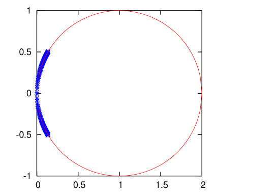
Figure 2: Lowest 202 eigenvalues of the overlap-Dirac operator at beta=5.85 on a $10^{3}20$ lattice of topological charge $Q=-2$. The eigenvalues cover a $\pi/3$ arc of the circle.

Table 1: Number of configurations in each topological sector.

$|Q|$	0	1	2	3
# of confs.	20	45	44	24

When the exact inverse of the overlap-Dirac operator is needed, we use the techniques described in Ref. Giusti:2002sm. For a given source vector $\eta$, we solve the equation

$$D_{m}\psi=\eta$$ (42)

by separating the left and right handed components as $\psi=P_{-}\psi+P_{+}\psi$ and solving two equations

$$P_{-}\psi = (P_{-}D^{\dagger}_{m}D_{m}P_{-})^{-1}P_{-}D^{\dagger}_{m}\eta,$$ (43)

$$P_{+}\psi = (P_{+}D_{m}P_{+})^{-1}(P_{+}\eta-P_{+}D_{m}P_{-}\psi),$$ (44)

consecutively. (The above equations apply for positive $Q$ and the same procedure applies with a replacement $P_{+}\leftrightarrow P_{-}$ for negative $Q$.) We use the conjugate gradient (CG) algorithm to invert the chirally projected matrices with the low-mode preconditioning with 20 lowest eigenmodes. With this low-mode preconditioning we gain about one order of magnitude speed-up of the CG solver (we need only 20-40 iterations for each $P_{\pm}\psi$.) for our smallest quark mass 0.0016, which corresponds to 2.6 MeV in the physical unit.

4 Low-mode dominance for the meson correlators

The inverse of the overlap-Dirac operator $D$ can be decomposed into the contributions from each eigenmode with eigenvalue $\lambda_{i}$ and eigenvector $v_{i}(x)$ as

$$D^{-1}_{m}(x,y)=\sum_{i=1}^{N_{\mathrm{low}}}\frac{1}{(1-\bar{a}m/2)\lambda_{i}+m}v_{i}(x)v_{i}^{\dagger}(y)+\Delta D^{-1}_{m}(x,y).$$ (45)

Here, the eigenmode decomposition is done incompletely, and the sum is truncated at some cutoff $N_{\mathrm{low}}$, which we set $N_{\mbox{\tiny low}}=200+|Q|$. The additional term $\Delta D^{-1}_{m}(x,y)$ represents the contribution from higher eigenmodes.

We expect that the low energy physics is dominated by the low-lying eigenmodes. Near the massless limit the lowest-lying eigenmodes play a dominant role as they are enhanced by a $1/\lambda_{i}$ factor, and especially the zero modes give divergent contribution in the quenched approximation. (In the unquenched case their occurrence is suppressed by the fermion determinant.) Sensitivity to the gauge field topology mostly comes from these low-lying eigenmodes. Therefore, the eigenmode decomposition (45) is expected to give a good approximation for low energy physics even if we ignore the higher mode contribution $\Delta D^{-1}_{m}(x,y)$. The cutoff $N_{\mathrm{low}}$ must be large enough for such approximation to cover the all relevant low-lying modes, and it depends on the pion mass and physical volume of the system. For massive fermions the eigenmodes below $\lambda_{i}\lesssim m$ become equally important, and we need larger $N_{\mathrm{low}}$ than in the massless limit.

On the other hand, the short distance physics could be affected by the higher eigenmodes. It can be seen by looking at the defining equation $\sum_{z}D_{m}(x,z)D_{m}^{-1}(z,y)=\sum_{i=1}^{N_{\mathrm{low}}}v_{i}(x)v_{i}^{\dagger}(y)+D_{m}(x,z)\Delta D_{m}^{-1}(z,y)=\delta(x,y)$ at $x=y$. Since the sum $\sum_{i=1}^{N_{\mathrm{low}}}v_{i}(x)v_{i}^{\dagger}(x)$ approaches monotonically to one when $N_{\mathrm{low}}$ is sent to the size of the matrix $N_{\mathrm{max}}$, the contribution from the remaining term $\Delta D_{m}^{-1}(x,y)$ becomes significant for $N_{\mathrm{low}}$ much smaller than $N_{\mathrm{max}}$. However, such a short distance correlation described by $\Delta D_{m}^{-1}(x,y)$ should be insensitive to the gauge field topology.

4.1 Connected correlators

First, let us consider the “connected” meson correlators

$$M_{i}(t)M_{i}(0)_{\mathrm{conn}} \equiv \sum_{\vec{x}}\bar{\psi}\Gamma_{i}\psi(\vec{x},t)\bar{\psi}\Gamma_{i}\psi(\vec{0},0)_{\mathrm{conn}}$$ (46)

$$= -\sum_{\vec{x}}\mbox{tr}\left(\Gamma_{i}D_{m}^{-1}(\vec{x},t;\vec{0},0)\Gamma_{i}D_{m}^{-1}(\vec{0},0;\vec{x},t)\right),$$

where $M_{i}$ denotes local operator corresponding to pseudo-scalar (PS), scalar (S), vector (V) and axial-vector (AV) currents, and $\Gamma_{i}$ denotes the corresponding gamma matrix, $\Gamma_{\mathrm{PS}}=i\gamma_{5}$, $\Gamma_{\mathrm{S}}=1$, $\Gamma_{\mathrm{V}}=i\gamma_{0}$, and $\Gamma_{\mathrm{AV}}=i\gamma_{5}\gamma_{0}$.

We calculate these correlators in two ways: one is an exact calculation with the conjugate gradient (CG) method and the other is the low-mode approximation

$$D^{-1}_{m}(x,y)\sim\sum_{i=1}^{200+|Q|}\frac{1}{(1-\bar{a}m/2)\lambda_{i}+m}v_{i}(x)v_{i}^{\dagger}(y),$$ (47)

where the higher eigenmode contributions are neglected. Comparison of them at $m$ = 0.0016, 0.0048, 0.008 ($\lesssim$ 13 MeV) is shown in Table 2, where maximal numerical difference between the two correlators in the region $7\leq t\leq 13$ is listed for each operator and topological sector. For the scalar and pseudo-scalar mesons, the approximation (47) does work well to 98–99.9% accuracy, while the lowest $200+|Q|$ modes are not enough to reproduce the vector and axial vector correlators. Figure 3 shows the pseudo-scalar and axial-vector correlators at $m$ = 0.008 and $|Q|=1$. We observe very good agreement for the pseudo-scalar correlator for wide region of $t$ (from 3 to 17), but the axial-vector case is much worse. This is probably because the axial-vector correlator is smaller in magnitude by a factor of $O(m)$, and therefore small fluctuation of eigenvectors is enhanced [24]. Figure 4 shows how the low-lying mode contributions saturate to the full correlators. We find that about 100 lowest eigenmodes suffice to approximate the full correlator to a very good accuracy. The plot is shown for $m=0.008$, but the saturation becomes even better for smaller quark masses.

Table 2: Comparison of the low-mode approximated “connected” correlators with their exact ones. The approximation uses the quark propagator (47) with $200+|Q|$ low-lying modes at $m$ = 0.0016, 0.0048, 0.008. The maximum deviation in $7\leq|t|\leq 13$ is shown. The number of configurations is given in Table 1.

$m=0.008$ ($\sim$ 13 MeV)	$|Q|=0$	$|Q|=1$	$|Q|=2$	$|Q|=3$
scalar	2.01%	1.49%	0.46%	0.44%
pseudo-scalar	1.19%	0.48%	0.28%	0.22%
vector	41.6%	258 %	259%	94.6%
axial-vector	28.4%	40.5%	24.3%	24.2%
$m=0.0048$ ($\sim$ 7.7 MeV)	$|Q|=0$	$|Q|=1$	$|Q|=2$	$|Q|=3$
scalar	1.57%	0.65%	0.16%	0.18%
pseudo-scalar	1.06%	0.33%	0.10%	0.08%
vector	28.9%	198 %	110%	104%
axial-vector	26.2%	38.6%	19.7%	18.3%
$m=0.0016$ ($\sim$ 2.6 MeV)	$|Q|=0$	$|Q|=1$	$|Q|=2$	$|Q|=3$
scalar	1.41%	0.08%	0.03%	0.03%
pseudo-scalar	0.95%	0.06%	0.04%	0.02%
vector	22.5%	149 %	157%	166%
axial-vector	21.5%	32.6%	20.4%	34.7%

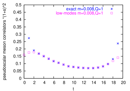
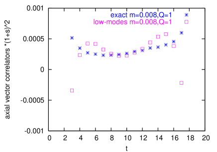
Figure 3: Pseudo-scalar (left) and axial-vector (right) correlators at $m$ = 0.008 and $|Q|=1$. The low-mode-approximated correlator (47) is compared with the corresponding exact one.

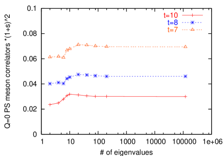
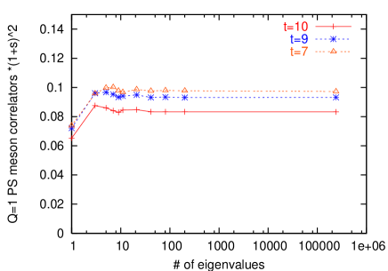
Figure 4: Saturation of the connected pseudo-scalar correlator for one sample configuration at $m=0.008$. Two plots are shown for $|Q|=0$ (left) and $|Q|=1$ (right). The rightmost points around 120,000 correspond to the exact correlator obtained by the CG method.

An advantage of the low-mode approximation (47) is that $D^{-1}_{m}(x,y)$ at any $x$ and $y$ is obtained without performing the CG inversion, so that one can easily average the source point over the space-time

$$\left\langle\sum_{\vec{x}}\bar{\psi}\Gamma_{i}\psi(\vec{x},t)\bar{\psi}\Gamma_{i}\psi(\vec{0},0)\right\rangle^{Q}_{\mathrm{conn}}\to\frac{1}{TL^{3}}\sum_{\vec{x}_{0},t_{0}}\left\langle\sum_{\vec{x}}\bar{\psi}\Gamma_{i}\psi(\vec{x},t+t_{0})\bar{\psi}\Gamma_{i}\psi(\vec{x}_{0},t_{0})\right\rangle^{Q}_{\mathrm{conn}}.$$ (48)

This so-called low-mode averaging dramatically reduces the fluctuation of the low-lying modes as shown in Figure 5, which is also reported in Ref. Giusti:2004yp. In practice we average only over $(L/2)^{3}\times(T/2)$ lattice points where the site index is an even number for each direction. Note that even after the low-mode averaging, the error from the truncation of the higher modes is negligible compared to the statistical error $\sim$ 15% in $Q=0$ sector and $\sim$ 5% in $Q\neq 0$ sectors in the range $7\leq t\leq 13$.

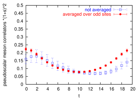
Figure 5: The pseudo-scalar correlator at $m=0.008$ and $|Q|=1$. Filled symbols denote the data with the low-mode averaging, while open symbols are not averaged.

4.2 Chiral condensates

Consider the low-mode contribution to the scalar and pseudo-scalar condensates for a fixed topological charge $Q$

$$\langle\bar{\psi}\psi(x)\rangle^{Q} = -\langle\mbox{tr}D_{m}^{-1}(x,x)\rangle^{Q}$$ (49)

$$= -\left\langle\mbox{tr}\left(\sum_{i=1}^{N_{\mbox{\tiny low}}}\frac{1}{(1-\bar{a}m/2)\lambda_{i}+m}v_{i}(x)v_{i}^{\dagger}(x)+\Delta D_{m}^{-1}(x,x)\right)\right\rangle^{Q},$$

$$\langle\bar{\psi}\gamma_{5}\psi(x)\rangle^{Q} = -\langle\mbox{tr}\gamma_{5}D_{m}^{-1}(x,x)\rangle^{Q}$$ (50)

$$= -\left\langle\mbox{tr}\left(\sum_{i=1}^{N_{\mbox{\tiny low}}}\frac{1}{(1-\bar{a}m/2)\lambda_{i}+m}\gamma_{5}v_{i}(x)v_{i}^{\dagger}(x)+\gamma_{5}\Delta D_{m}^{-1}(x,x)\right)\right\rangle^{Q}.$$

For the scalar condensates, it is known that $\Delta D_{m}^{-1}(x,x)$ includes unwanted additive ultraviolet divergences [25]

$$\langle\mbox{tr}D_{m}^{-1}(x,x)\rangle^{Q}=\frac{6}{(1+s)a^{3}}+C_{2}\frac{m}{a^{2}}+C_{1}\frac{m^{2}}{a}+\Sigma_{Q}(\mu^{\prime})+O(\epsilon^{4}),$$ (51)

where $C_{2}$ and $C_{1}$ are unknown constants. The first term comes from the modification of the chiral symmetry in the Ginsparg-Wilson relation [10], $\gamma_{5}D^{-1}(x,y)+D^{-1}(x,y)\gamma_{5}=\bar{a}\delta_{x,y}$, at $x=y$. If $N_{\mathrm{low}}$ is large enough, the higher mode contribution $\Delta D_{m}^{-1}(x,x)$ should be insensitive to the link variables $U_{\mu}(y)$ separated large enough from $x$ and thus to the global structure of the gauge field configuration, such as the topological charge. We, therefore, expect that such contribution vanishes in the difference between different topological sectors,

$$-(\langle\bar{\psi}\psi(x)\rangle^{Q}-\langle\bar{\psi}\psi(x)\rangle^{0}).$$ (52)

In other words this difference should be well described only by the low-lying eigenmodes. In fact we observe such a low-mode saturation as shown in Figures 6 and 7, while the individual condensate $-\langle\bar{\psi}\psi(x)\rangle^{Q}$ is not saturated.

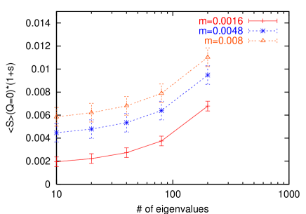
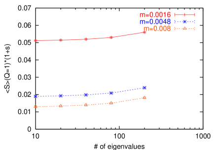
Figure 6: Low-mode saturation for $-\langle\bar{\psi}\psi\rangle^{Q}$. Data are averaged over 20 gauge configurations of $Q=0$ (left) and $Q=1$ (right).

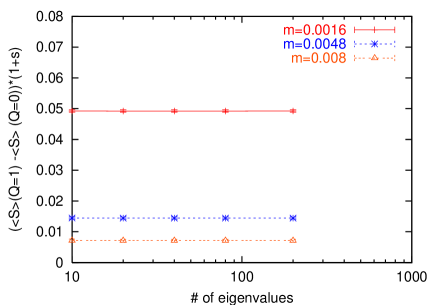
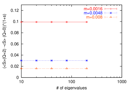
Figure 7: Low-mode saturation for $-(\langle\bar{\psi}\psi\rangle^{Q}-\langle\bar{\psi}\psi\rangle^{0})$ averaged over 20 configurations at $Q=1$ (left) and $Q=2$ (right).

For the pseudo-scalar condensate, we do not have to take care of the higher modes because the condensate is determined only by the zero modes and the contributions from other eigenmodes cancel because of the orthogonality among different eigenvectors. As shown in Figure 8, our data with $N_{\mbox{\tiny low}}=200+|Q|$ low-modes perfectly agree with the theoretical expectation

$$-\langle\bar{\psi}\gamma_{5}\psi\rangle_{Q}=\frac{Q}{mV}.$$ (53)

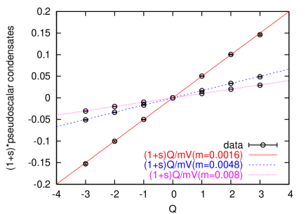
Figure 8: Pseudo-scalar condensates approximated with $N_{\mbox{\tiny low}}=200+|Q|$ low-modes. The lines represent the expectation (53).

4.3 Disconnected correlators

Here we discuss the expectation value of the “disconnected” diagrams for a fixed topological charge. As in the case of the connected diagram, we expect

$$\langle M_{i}(t)M_{i}(0)\rangle_{\mathrm{disc}}^{Q} \equiv \left\langle\sum_{\vec{x}}\bar{\psi}\Gamma_{i}\psi(\vec{x},t)\bar{\psi}\Gamma_{i}\psi(\vec{0},0)\right\rangle_{\mathrm{disc}}^{Q}$$ (54)

$$= \left\langle\sum_{\vec{x}}\mbox{tr}\left(\Gamma_{i}D_{m}^{-1}(\vec{x},t;\vec{x},t)\right)\mbox{tr}\left(\Gamma_{i}D_{m}^{-1}(\vec{0},0;\vec{0},0)\right)\right\rangle^{Q},$$

$$\stackrel{{\scriptstyle t\gg 0}}{{\longrightarrow}} \left\langle\sum_{\vec{x}}\mbox{tr}\left(\Gamma_{i}\sum_{i=1}^{200+|Q|}\frac{1}{(1-\bar{a}m/2)\lambda_{i}+m}v_{i}(x)v_{i}^{\dagger}(x)\right)\right.$$

$$\left.\times\mbox{tr}\left(\Gamma_{i}\sum_{i=1}^{200+|Q|}\frac{1}{(1-\bar{a}m/2)\lambda_{i}+m}v_{i}(0)v_{i}^{\dagger}(0)\right)\right\rangle^{Q}$$

$$+ 2\left\langle\mbox{tr}\left(\Gamma_{i}\Delta D_{m}^{-1}(x,x)\right)\right\rangle^{\prime}$$

$$\times\left\langle\mbox{tr}\left(\Gamma_{i}\sum_{i=1}^{200+|Q|}\frac{1}{(1-\bar{a}m/2)\lambda_{i}+m}v_{i}(0)v_{i}^{\dagger}(0)\right)\right\rangle^{Q}$$

$$+ \left[\left\langle\mbox{tr}\left(\Gamma_{i}\Delta D_{m}^{-1}(x,x)\right)\right\rangle^{\prime}\right]^{2},$$

where $x=(\vec{x},t)$. We assume that higher modes’ contribution does not have correlation with any local operator $O(y)$ separated enough from $x$, i.e.

$$\langle\Delta D_{m}^{-1}(x,x)O(y)\rangle^{Q}\stackrel{{\scriptstyle|x-y|\gg 0}}{{\longrightarrow}}\langle\Delta D_{m}^{-1}(x,x)\rangle^{\prime}\times\langle O(y)\rangle^{Q},$$ (55)

where the expectation value $\langle\cdots\rangle^{\prime}$ represents insensitivity to the topological charge. We also use the translational invariance $\langle O(x)\rangle=\langle O(0)\rangle$. Unlike in the “connected” case, we cannot check the low-mode dominance by explicitly computing the exact correlators because the numerical cost is too expensive. However, for the pseudo-scalar disconnected diagram $\langle\mbox{tr}\gamma_{5}\Delta D_{m}^{-1}(x,x)\rangle^{\prime}$ vanishes because $\Delta D_{m}^{-1}(x,x)$ does not contain the zero modes.

In fact, as Figure 9 shows, we find good saturation with the lowest 200 eigenmodes for the pseudo-scalar disconnected correlators. Similar results were also obtained previously in the study of the $\eta^{\prime}$ propagator with the Wilson fermion [26] and with the overlap fermion [27].

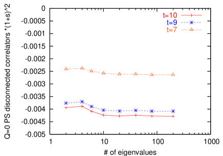
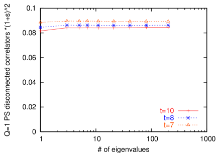
Figure 9: Saturation of the pseudo-scalar disconnected correlators for one sample configuration at $m=0.008$ for $Q=0$ (left) and $Q=1$ (right).

5 Extraction of the low energy constants from the meson correlators

5.1 $F_{\pi}$ from the axial-vector correlator

The axial-vector current correlator (35) is most sensitive to $F_{\pi}$ and not contaminated by the parameters $m_{0}$ and $\alpha$. The problem is, however, that the low-mode dominance does not hold, and we have to solve the quark propagators exactly. Hence, the statistical noise could become a problem as we cannot average the source point over space-time. Our strategy is to treat data at different quark masses and different topologies at the same time to reduce such large statistical errors.

We use the local axial-current $A_{\mu}^{a}(x)=\bar{\psi}(x)\gamma_{5}\gamma_{\mu}(\tau^{a}/2)\psi(x)$, constructed from the overlap fermion field $\psi(x)$. Since it is not the conserved current corresponding to the lattice chiral symmetry, (finite) renormalization is needed to relate it to the continuum axial-vector current. To calculate the $Z_{A}$ factor non-perturbatively, we follow the method applied in Refs. Giusti:2001yw,Giusti:2001pk. Namely, we calculate

$$aR_{\rho}(t)\equiv\frac{a\sum_{\vec{x}}\langle\bar{\nabla}_{0}A^{a}_{0}(\vec{x},t)P^{a}(0,0)\rangle}{\sum_{\vec{x}}\langle P^{a}(\vec{x},t)P^{a}(0,0)\rangle},$$ (56)

where $\bar{\nabla}_{0}$ denotes a symmetric lattice derivative. The pseudo-scalar density $P^{a}(x)$ must be the chirally improved one $\bar{\psi}(\tau^{a}/2)\gamma_{5}(1-\frac{\bar{a}}{2}D)\psi$ associated with the exact chiral symmetry on the lattice. For the on-shell matrix elements such as the one considered here, one can use the equation of motion to replace the $\bar{a}D$ term by $-am/(1-\bar{a}m/2)$, which is negligible for our quark masses. We therefore use the local operator for $P^{a}(x)$.

The ratio (56) turns out to be insensitive to topology as shown in Figure 10. Fitting the average of $R_{\rho}(t)$ over all topological sectors with a constant in the range $7\leq t\leq 13$, we obtain the results for

$$a\rho(ma)\equiv\frac{a\langle\bar{\nabla_{\mu}}A^{a}_{\mu}(x)P^{a}(0)\rangle}{\langle P^{a}(x)P^{a}(0)\rangle}=\frac{2ma}{Z_{A}}+O(a^{2})$$ (57)

at four quark masses $m$ = 0.0016, 0.0048, 0.008, 0.0160, which are shown in Figure 11. With a quadratic fit we obtain

$$a\rho(ma)=0.00001(2)+1.390(14)(ma)-0.19(74)(ma)^{2}.$$ (58)

The constant term is perfectly consistent with zero and we can extract $Z_{A}$ from the linear term as $Z_{A}$ = 1.439(15) , which is consistent with the value $Z_{A}$ = 1.448(4) reported in Ref. Bietenholz:2004wv which was done with the same $\beta$ and $s$.

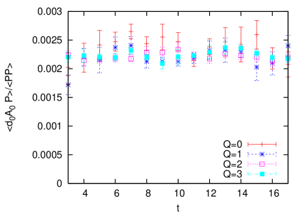
Figure 10: $aR_{\rho}(t)$ at $m=0.0016$. Data for topological sectors $|Q|$ = 0, 1, 2, and 3 are shown.

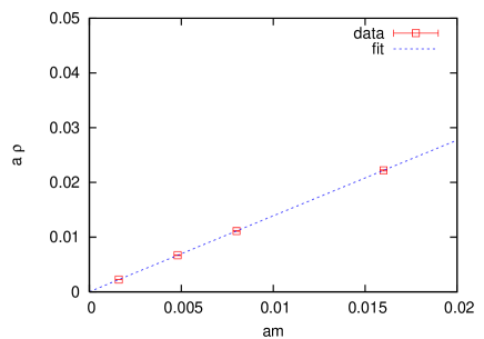
Figure 11: $a\rho$ as a function of the bare quark mass. Dashed line is a result of the quadratic fit: $a\rho=0.00001+1.390(ma)-0.19(ma)^{2}$.

We now compare the renormalized axial-vector correlation function with the QChPT result

$$2Z_{A}^{2}\sum_{\vec{x}}\langle A_{0}(\vec{x},t)A_{0}(0,0)\rangle^{Q}=2\left(\frac{F_{\pi}^{2}}{T}+2m\Sigma_{|Q|}(\mu)Th_{1}(|t/T|)\right).$$ (59)

From the constant term we can determine $F_{\pi}$, while $\Sigma$ has to be extracted from the small $t$ dependence. In Ref. Bietenholz:2003bj it is reported that the correlators suffer from large statistical fluctuation at $|Q|=0$ and other topological sectors are insensitive to $\Sigma$. We observed similarly large statistical noise as shown in Figure 12, but it turned out that two-parameter ($F_{\pi}$ and $\Sigma$) fitting does work well when we treat the data of different topology and fermion masses simultaneously.

As Figure 12 shows, our data at $m$ = 0.0016, 0.0048, 0.008 in the $|Q|\leq 1$ sectors are well described by the QChPT formula (59). A simultaneous fit in the range $7\leq t\leq 13$ yields $F_{\pi}$ = 98.3(8.3) MeV and $\Sigma^{1/3}$ = 259(50) MeV with $\chi^{2}/\mbox{dof}$ = 0.19. These results are stable under a change of the fit range: $(F_{\pi},\Sigma^{1/3})$ = (98.8(8.3) MeV, 261(47) MeV) and (99.2(8.3) MeV, 261(45) MeV) for $8\leq t\leq 12$ and $9\leq t\leq 11$, respectively. The result for $F_{\pi}$ is in agreement with that of the previous work [17], 102(4) MeV. The authors of Bietenholz:2003bj quoted a slightly larger value $\sim$ 130 MeV.

The correlators at $|Q|$ = 2 do not agree well with the above fit parameters as shown in Figure 13. As discussed in Section 2 it may indicate that the topological sector $|Q|$ = 2 is already too large to apply the QChPT in the $\epsilon$-regime.

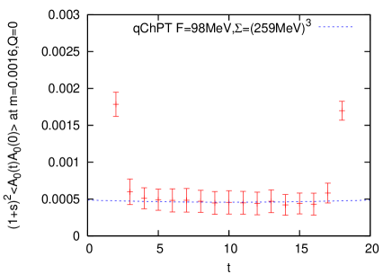
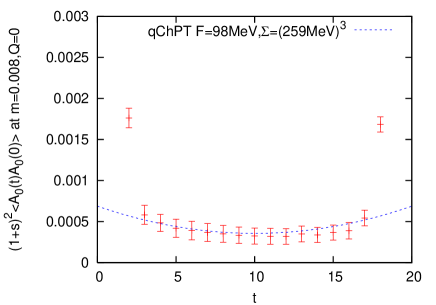
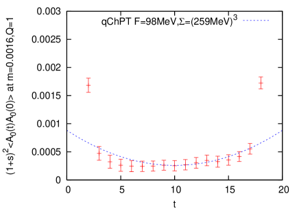
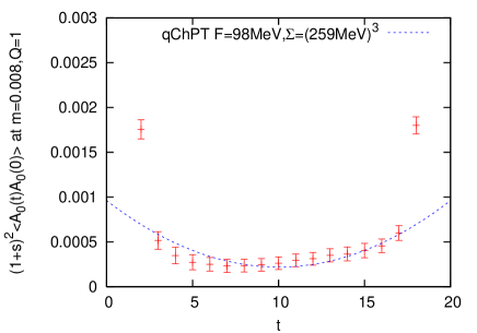
Figure 12: Axial-vector current correlators at $m$ = 0.0016 (left) and 0.008 (right) for $|Q|$ = 0 (top) and 1 (bottom). The dashed lines are the result of simultaneous fitting of the data for $Q$ = 0 and 1 at $m$ = 0.0016, 0.0048, 0.008 in the region $7\leq t\leq 13$.

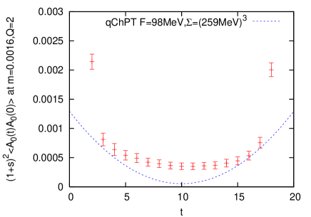
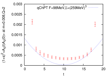
Figure 13: Axial-vector current correlators at $m$ = 0.0016 (left) and 0.008 (right) for $|Q|$ = 2. The dashed lines are the QChPT prediction with parameters determined through $|Q|$ = 0 and 1 sectors.

5.2 $\Sigma$, $\Sigma_{\mathrm{eff}}$ and $\alpha$ from connected S and PS correlators

As discussed in the previous section, the scalar and pseudo-scalar connected correlators are approximated rather precisely only with the lowest 200$+|Q|$ eigen-modes at small quark masses ($m$ = 2.6–13 MeV). In this way we measure the scalar (pseudo-scalar) correlators

$$\langle\mathcal{S}(t)\rangle^{Q}\equiv-2\sum_{\vec{x}}(1+s)^{2}\langle S^{3}(x)S^{3}(0)\rangle^{Q}_{\mathrm{low-modes}},$$ (60)

$$\langle\mathcal{P}(t)\rangle^{Q}\equiv 2\sum_{\vec{x}}(1+s)^{2}\langle P^{3}(x)P^{3}(0)\rangle^{Q}_{\mathrm{low-modes}},$$ (61)

for the topological sectors $1\leq|Q|\leq 3$ ($0\leq|Q|\leq 3$) at $m$ = 0.0016, 0.0032, 0.0048, 0.0064, and 0.008, in which the error from higher mode truncation is estimated to be only $\lesssim 1$ %, which can be ignored compared to statistical errors. We take an average of the source point over $(L/2)^{3}\times(T/2)$ lattice sites.

To fit our data with the one-loop QChPT formulae (26) and (27), we have to determine five parameters in these formulae: $F_{\pi}$, $\Sigma$, $\Sigma_{\mathrm{eff}}$, $m_{0}^{2}$ and $\alpha$. Since the sensitivity for $F_{\pi}$ is weak with these correlators, we use the jackknife samples of $F_{\pi}$ obtained through the axial-vector current correlator, $F_{\pi}$ = 98.3(8.3) MeV. Unfortunately, there still remain too many parameters to fit with QChPT expressions. Therefore, to determine $m_{0}^{2}$ we use the relation (6) and input the value of topological susceptibility $\chi\equiv\langle Q^{2}\rangle/V$ from a recent work [31] as $r_{0}^{4}\chi$ = 0.059(3). It gives $m_{0}$ = 940(80)(23) MeV, where the second error reflects the error of $r_{0}^{4}\chi$.

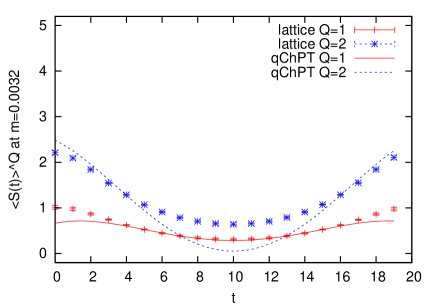
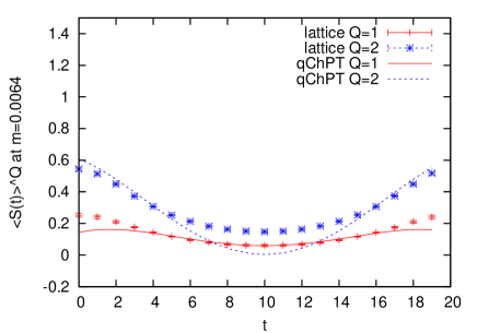
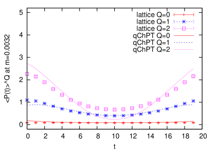
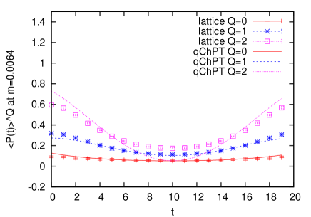
Figure 14: Scalar (top) and pseudo-scalar (bottom) correlators at $m$ = 0.0032 (left) and 0.0064 (right). The dotted lines are the fit results with all available mass parameters $m$ = 0.0016, 0.0032, 0.0064 and 0.008 for topological charges 0 and 1.

Using these inputs, we fit the correlators (60) and (61) in the range $7\leq t\leq 13$ at different $Q$ and $m$ simultaneously. Figure 14 shows the correlators with fit curves. For $|Q|\leq 1$, the data at all available quark masses $m$ = 0.0016, 0.0032, 0.0064 and 0.008 are fitted well, and we actually obtain $\chi^{2}/\mathrm{dof}$ $\sim$ 0.7. (Note that the correlations between different $t$’s, $m$’s and channels (PS and S) are not taken into account.) Our fit results are $\Sigma^{1/3}$ = 257 $\pm$ 14 $\pm$ 00 MeV, which is consistent with Ref. Bietenholz:2003mi, $\Sigma_{\mathrm{eff}}^{1/3}$ = 271 $\pm$ 12 $\pm$ 00 MeV, and $\alpha$ = $-$4.5 $\pm$ 1.2 $\pm$ 0.2, where the first error is the statistical error and the second one is from uncertainty of $\langle Q^{2}\rangle$. They are insensitive to the choice of the fit range. The central values vary only slightly (for instance, $\pm$ 1 MeV for $\Sigma^{1/3}$ and $\Sigma_{\mathrm{eff}}^{1/3}$) by choosing shorter fitting ranges $8\leq t\leq 12$ and $9\leq t\leq 11$.

From the ratio $\Sigma_{\mathrm{eff}}/\Sigma$ we can identify the size of the NLO correction in the $\epsilon$ expansion. To the one-loop level, it is written as

$$\frac{\Sigma_{\mathrm{eff}}}{\Sigma}=1+\frac{1}{N_{c}F_{\pi}}\left(m_{0}^{2}\bar{G}(0)+\alpha\bar{\Delta}(0)\right),$$ (62)

where the parameters $\bar{G}(0)$ and $\bar{\Delta}(0)$ are regularization dependent. For this ratio we obtain 1.163(59), which indicates that the $\epsilon$ expansion is actually converging.

We obtain large negative value for $\alpha$, which is also reported in Refs. Bietenholz:2005kq and Shcheredin:2005ma. These results contradict with a previous precise calculation [35], which obtained a small value $\alpha$ = 0.03(3). If we instead assume $\alpha$ = 0, and fit $F_{\pi}$ as a free parameter, we obtain $F_{\pi}$ = 136.9(5.3) MeV and $\Sigma$ and $\Sigma_{\mathrm{eff}}$ are almost unchanged. (Detailed numbers are summarized in Table 3.) Therefore, there is an apparent inconsistency in the determination of $F_{\pi}$ between the axial-vector and (pseudo-)scalar correlators if $\alpha\sim 0$ is assumed. A possible cause is that $|Q|=1$ is not small enough to derive the partition function Eq.(5) (See Appendix). Eq.(6) may also have a systematic error due to finite $V$ as well as finite $a$.

The data at higher topological charge, $|Q|$ = 2, are also plotted in Figure 14. They do not quite agree with expectations from the QChPT shown by dashed curves in the plots. A simultaneous fit with all the data including $|Q|$ = 0, 1 and 2 gives a bad $\chi^{2}/\mathrm{dof}$ ($\simeq$ 12). This problem of higher topological charge also happens for the axial-vector correlator as discussed in the previous subsection.

5.3 Scalar condensate

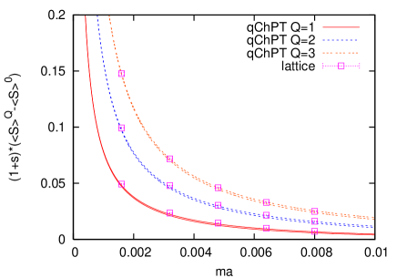
Figure 15: $-(\langle\bar{\psi}\psi\rangle^{Q}-\langle\bar{\psi}\psi\rangle^{0})$ as a function of quark mass. Data points are at $m$ = 0.0016, 0.0032, 0.0048, 0.0064, 0.008. The lines are QChPT predictions with $\Sigma_{\mathrm{eff}}^{1/3}$ = 271(12) MeV.

The free parameter in the scalar condensate is $\Sigma_{\mathrm{eff}}$ as seen in (8) and (9). To avoid the problem of ultraviolet divergence we compare a difference $-(\langle\bar{\psi}\psi\rangle^{Q}-\langle\bar{\psi}\psi\rangle^{0})$ with the QChPT result $\Sigma_{Q}(\mu^{\prime})-\Sigma_{Q=0}(\mu^{\prime})$. We use the low-mode approximation with 200+$|Q|$ eigenmodes, and the low-mode averaging is done as in the meson correlators. Figure 15 shows the difference as a function of quark mass for $|Q|$ = 1, 2 and 3. We find that the lattice data agree remarkably well with the QChPT expectation with $\Sigma_{\mathrm{eff}}$ = 271(12) MeV as determined from the (pseudo-)scalar connected correlator even in higher topological sectors. In fact, if we fit the scalar condensate with $\Sigma_{\mathrm{eff}}$ as a free parameter, we obtain 256(14) MeV which is consistent with the result above.

5.4 Disconnected PS correlators

We also measure the disconnected pseudo-scalar correlators, which is made possible with the low-mode approximation. The saturation with 200+$|Q|$ lowest-lying mode is quite good for the pseudo-scalar channel as discussed in Section 4.3.

In the QChPT it is written as

$$\langle\mathcal{P}^{d}(t)\rangle^{Q} \equiv \int\!d^{3}x\,(1+s)^{2}\langle 2P^{3}(x)P^{3}(0)-P^{0}(x)P^{0}(0)\rangle^{Q}$$ (63)

$$= \int\!d^{3}x\,(1+s)^{2}\left[C_{P}^{d}-\frac{\Sigma^{2}}{2F_{\pi}^{2}}\left(\frac{d_{+}}{N_{c}}(m_{0}^{2}\bar{G}(x)+\alpha\bar{\Delta}(x))-e_{+}\bar{\Delta}(x)\right)\right],$$

where

$$C_{P}^{d} = \frac{Q^{2}}{m^{2}V^{2}},$$ (64)

$$d_{+} = -4\left(1+\frac{Q^{2}}{\mu^{2}}\right),$$ (65)

$$e_{+} = -2\left(\left(\frac{\Sigma_{Q}(\mu)}{\Sigma}\right)^{\prime}-\frac{\Sigma_{Q}(\mu)}{\mu\Sigma}\right).$$ (66)

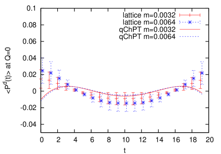
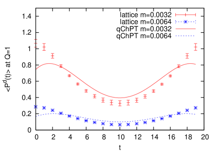
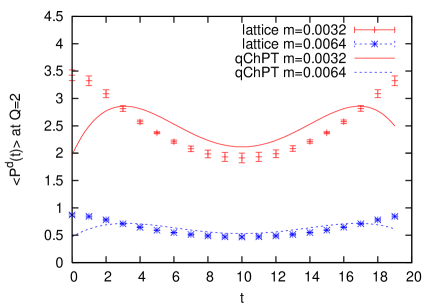
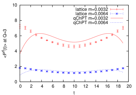
Figure 16: Disconnected pseudo-scalar correlators in the $0\leq|Q|\leq 3$ sectors at $m$ = 0.0032 and 0.0064. The curves represent the results of QChPT with $\Sigma^{1/3}$ = 257 MeV, $F_{\pi}$ = 98.3 MeV, $m_{0}$ = 940 MeV and $\alpha$ = $-$4.5.

In Figure 16 lattice data for topological sectors $|Q|$ = 0–3 are shown at two representative quark masses $m$ = 0.0032 and 0.0064. The QChPT predictions are plotted with the parameters determined through the axial-vector and (pseudo-)scalar connected correlators: $\Sigma^{1/3}$ = 257 MeV, $F_{\pi}$ = 98.3 MeV, $m_{0}$ = 940 MeV, and $\alpha$ = $-$4.5. We observe that the agreement is marginal, though the correlator’s magnitude and shape are qualitatively well described. Instead, if we fit the disconnected correlator with $\Sigma$ and $\alpha$ as free parameters while fixing $F_{\pi}$ and $m_{0}$ to the same value, we obtain $\Sigma^{1/3}$ = 227(32) MeV and $\alpha$ = $-$3.5(1.2), which are statistically consistent with those input numbers. Therefore, we conclude that both the connected and disconnected correlators are consistently described by the QChPT in the $\epsilon$-regime. Details of the fit results are listed in Table 3.

Table 3: Summary of the fitting results. The first column denotes the topological sectors used in the fit. The values in $[\cdots]$ are input parameters. The first error is statistical. The second and third errors reflect the uncertainty in the input parameters, $\langle Q^{2}\rangle$ and $F_{\pi}$, respectively.

correlators	$F_{\pi}$(MeV)	$\Sigma^{1/3}$ (MeV)	$\Sigma_{\mathrm{eff}}^{1/3}$ (MeV)	$\alpha$	$m_{0}$ (MeV)	$\chi^{2}/\mathrm{dof}$
axial vector
$|Q|=0$	98(17)	279(65)				0.02
$0\leq|Q|\leq 1$	98.3(8.3)	259(50)				0.19
$0\leq|Q|\leq 2$	117.9(4.3)	335(16)				2.8
connected PS+S
$0\leq|Q|\leq 1$	[98.3(8.3)]	257(14)(00)	271(12)(00)	$-$4.5(1.2)(0.2)	[940(80)(23)]	0.7
$0\leq|Q|\leq 1$	136.9(5.3)(0.9)	250(13)(00)	258(11)(00)	[0]	[674(26)(16)]	0.3
$0\leq|Q|\leq 2$	[98.3(8.3)]	258(12)(00)	264(11)(00)	$-$3.8(0.5)(0.2)	[940(80)(23)]	11.8
disconnected PS
$0\leq|Q|\leq 1$	[98.3(8.3)]	227(32)(00)		$-$3.5(1.2)(0.3)	[940(80)(23)]	1.0
$0\leq|Q|\leq 1$	125.7(5.6)(0.9)	223(29)(00)		[0]	[734(33)(14)]	0.7
$0\leq|Q|\leq 2$	[98.3(8.3)]	229(33)(00)(03)		$-$3.6(0.2)(0.3)(1.0)	[940(80)(23)]	1.0
$0\leq|Q|\leq 2$	135.0(4.9)(1.4)	237(32)(00)		[0]	[684(25)(13)]	1.7
$0\leq|Q|\leq 3$	[98.3(8.3)]	229(33)(01)(05)		$-$3.6(0.1)(0.2)(0.8)	[940(80)(23)]	1.0
$0\leq|Q|\leq 3$	139.3(4.1)(1.4)	244(32)(00)		[0]	[663(19)(12)]	1.9
scalar condensate ($\langle\bar{\psi}\psi\rangle^{0}-\langle\bar{\psi}\psi\rangle^{Q}$)
$1\leq|Q|\leq 3$			256(14)			1.2

6 Conclusions

In the $\epsilon$-regime of ChPT, the meson correlators are largely affected by the fermion zero-mode, and thus by the topological charge of background gauge field. This expectation from the effective field theory is explicitly confirmed by a first-principles calculation of lattice QCD using the overlap Dirac operator, with which we can preserve the exact chiral symmetry at finite lattice spacing.

To reach the $\epsilon$-regime we need small quark masses to satisfy the condition $M_{\pi}L\lesssim 1$. This can be achieved by using the eigenmode decomposition of the fermion propagator. Then, the connected scalar and pseudo-scalar correlators are precisely reproduced by using only 200 low-lying eigenmodes. This number would be unchanged even when we decrease the lattice spacing, as far as the physical volume is kept fixed to $\sim(1.2\mbox{~{}fm})^{3}\times(2.4\mbox{~{}fm})$, since the small eigenvalue distribution depends only on a combination $\lambda\Sigma V$ in the $\epsilon$-regime. The $a\to 0$ limit affects higher modes only, which are irrelevant to the low energy dynamics. For those connected meson correlators the small quark mass regimes are reached without extra computational costs, and we can also employ the low-mode averaging technique to substantially reduce the statistical noise due to near-zero mode contributions. For the axial-vector current correlator, on the other hand, the saturation by low-lying modes is much worse and we had to treat them exactly using the (costly) CG solver. We also investigate the disconnected pseudo-scalar correlator using the low-lying mode approximation. The disconnected diagrams are usually very expensive as they need many fermion inversions, but with this approximation they are obtained without extra costs. We confirm that the disconnected pseudo-scalar correlator is well saturated by 200 low-lying eigenmodes for our lattice.

Remarkable $Q$ and $\mu$ dependences of the quenched ChPT are well reproduced by our lattice calculation at $\beta$ = 5.85 on a 10${}^{3}\times$20 lattice. Then we are able to extract some of the low energy constants: $F_{\pi}$, $\Sigma$, $m_{0}^{2}$ and $\alpha$. The last two describe the artifact of the quenched approximation. Fitting our data for meson correlators simultaneously at different quark masses and topological charges, we obtain $F_{\pi}$ = 98.3(8.3) MeV, $\Sigma^{1/3}$ = 257(14)(00) MeV ($\Sigma_{\mathrm{eff}}^{1/3}$ = 271(12)(00) MeV), $m_{0}$ = 940(80)(23) MeV, and $\alpha$ = $-$4.5(1.2)(0.2), from the connected correlators with $|Q|\leq 1$. In these numerical results the second error reflects the error of $\langle Q^{2}\rangle$. We also obtain consistent results from disconnected pseudo-scalar correlator and the chiral condensate.

Despite such remarkable success of QChPT, we also find problems. First, the correlators in $|Q|\geq 2$ sectors are not well fitted by the parameters determined at $|Q|\leq 1$. This may indicate a problem of the $\epsilon$-expansion in QChPT, which comes from the fact that the partition function at a fixed topology can be justified only for $|Q|\ll\langle Q^{2}\rangle$. Since $\langle Q^{2}\rangle$ is proportional to $V$, this condition is relaxed on larger lattices. It is therefore interesting to extend our study to larger volumes. Secondly, the numerical result for $\alpha$ is rather large and negative. Such a large value may pose a question on the validity of the partition function (5). Previous lattice calculations, e.g. [35], indicated the value consistent with zero and our result is clearly inconsistent with them. If we assume $\alpha$ = 0, then our data prefer larger value of $F_{\pi}\simeq$ 130 MeV, which contradicts with the result of the axial-vector correlator. Our calculations are, of course, not free from other systematic errors due to higher order terms in QChPT, finite lattice spacing, etc. However, because of the exact chiral symmetry the finite lattice spacing error does not spoil the consistency with (Q)ChPT, while the extracted parameters are contaminated.

Once these problems are (positively) solved, the lattice simulation in the $\epsilon$-regime could become a strong alternative to the conventional large volume (or large quark mass) simulations. A clear advantage is that the small enough quark masses can be reached and there is practically no question on the applicability of ChPT. Obviously, the dynamical simulations in the $\epsilon$-regime are most desirable. With the overlap fermion we do not see any fundamental problem, since the overlap-Dirac operator is well-conditioned even in the massless limit, though it is numerically too expensive on the current-generation machines.

In this appendix we derive the partition function at a fixed topological charge (5). It is obtained from the partition function (1) by Fourier transforming in $\theta$.

$$Z_{Q}(M) \equiv \frac{1}{2\pi}\int^{\pi}_{-\pi}\!d\theta e^{i\theta Q}Z(\theta,M)$$ (67)

$$= \frac{1}{2\pi}\int^{\pi}_{-\pi}\!d\theta\int dU^{\prime}_{0}d\xi(\mbox{Sdet}U_{0}^{\prime})^{Q}\exp\left[-\int d^{4}x\left(\mathcal{L}+i\frac{\sqrt{2}Q}{F_{\pi}V}\Phi_{0}\right)\right]$$

$$= \frac{1}{2\pi}\int^{\pi}_{-\pi}\!d\theta\int dU^{\prime}_{0}d\xi(\mbox{Sdet}U_{0}^{\prime})^{Q}\exp\left[-\frac{Vm_{0}^{2}}{2N_{c}}\left(\Phi_{0}^{\prime}-\frac{F_{\pi}\theta}{\sqrt{2}}\right)^{2}-\frac{\sqrt{2}iQ}{F_{\pi}}\left(\Phi_{0}^{\prime}-\frac{F_{\pi}\theta}{\sqrt{2}}\right)\right]$$

$$\times\exp\left[\frac{m\Sigma V}{2}\mbox{Str}(U_{0}^{\prime}+U_{0}^{\prime-1})\right.$$

$$\left.\;\;+\int d^{4}x\left(-\frac{1}{2}\mbox{Str}(\partial_{\mu}\xi\partial_{\mu}\xi)-\frac{m_{0}^{2}}{2N_{c}}(\mbox{Str}\xi)^{2}-\frac{\alpha}{2N_{c}}(\partial_{\mu}\mbox{Str}\xi)^{2}\right)\right]$$

$$= \frac{1}{\sqrt{2\pi\langle Q^{2}\rangle}}e^{-Q^{2}/2\langle Q^{2}\rangle}\int dU^{\prime}_{0}d\xi(\mbox{Sdet}U^{\prime}_{0})^{Q}\exp\left[\frac{m\Sigma V}{2}\mbox{Str}(U^{\prime}_{0}+U^{\prime-1}_{0})\right.$$

$$+\left.\int d^{4}x\left(-\frac{1}{2}\mbox{Str}(\partial_{\mu}\xi\partial_{\mu}\xi)-\frac{m_{0}^{2}}{2N_{c}}(\mbox{Str}\xi)^{2}-\frac{\alpha}{2N_{c}}(\partial_{\mu}\mbox{Str}\xi)^{2}\right)+O(\epsilon^{4})\right],$$

where we use

$$U = U_{0}e^{i\sqrt{2}\xi/F_{\pi}},$$ (68)

$$\Phi_{0} \equiv \frac{F_{\pi}}{\sqrt{2}}\mbox{Str}(-i\ln U_{0}),$$ (69)

$$U_{0}^{\prime} = U_{\theta}U_{0},$$ (70)

$$e^{iQ\theta} = (\mbox{Sdet}U_{0}^{\prime})^{Q}\exp\left(-\int d^{4}x\frac{\sqrt{2}iQ}{F_{\pi}V}\Phi_{0}\right),$$ (71)

$$\Phi_{0}^{\prime} \equiv \frac{F_{\pi}}{\sqrt{2}}\mbox{Str}(-i\ln U_{0}^{\prime})=\Phi_{0}+\frac{F_{\pi}\theta}{\sqrt{2}}.$$ (72)

In the last line of (67), we perform $\theta$ integral as a Gaussian;

$$\frac{1}{2\pi}\int^{\pi}_{-\pi}d\theta\exp\left[-\frac{Vm_{0}^{2}F_{\pi}^{2}}{4N_{c}}\left(\theta-\frac{\sqrt{2}}{F_{\pi}}\Phi_{0}^{\prime}\right)^{2}+iQ\left(\theta-\frac{\sqrt{2}}{F_{\pi}}\Phi_{0}^{\prime}\right)\right]$$ (73)

$$= \exp\left(-\frac{Q^{2}}{2\langle Q^{2}\rangle}\right)\frac{1}{2\pi}\int^{\pi}_{-\pi}d\theta^{\prime}\exp\left[-\frac{\langle Q^{2}\rangle}{2}\left(\theta^{\prime}-\frac{iQ}{\langle Q^{2}\rangle}\right)^{2}\right]$$

$$\sim \frac{1}{\sqrt{2\pi\langle Q^{2}\rangle}}\exp\left(-\frac{Q^{2}}{2\langle Q^{2}\rangle}\right),$$

where $\langle Q^{2}\rangle=Vm_{0}^{2}F_{\pi}^{2}/2N_{c}$ and $\theta^{\prime}=\theta-\sqrt{2}\Phi^{\prime}_{0}/F_{\pi}$. To justify this Gaussian integral, we need a condition $|Q|/\langle Q^{2}\rangle\ll 1$, otherwise the integral (73) should depend on $\Phi_{0}^{\prime}$, which means that $\Phi_{0}^{\prime}$ and $\theta$ can not be treated independently and the partition function Eq.(5) is not valid. On our lattice with $\langle Q^{2}\rangle=4.34(22)$, this condition becomes questionable for $|Q|\neq 0$.

References

- [1] J. Gasser and H. Leutwyler, Annals Phys. 158, 142 (1984).
- [2] J. Gasser and H. Leutwyler, Phys. Lett. B 188, 477 (1987).
- [3] F. C. Hansen, Nucl. Phys. B 345, 685 (1990).
- [4] F. C. Hansen and H. Leutwyler, Nucl. Phys. B 350, 201 (1991).
- [5] P. H. Damgaard, M. C. Diamantini, P. Hernandez and K. Jansen, Nucl. Phys. B 629, 445 (2002) [arXiv:hep-lat/0112016].
- [6] P. H. Damgaard, P. Hernandez, K. Jansen, M. Laine and L. Lellouch, Nucl. Phys. B 656, 226 (2003) [arXiv:hep-lat/0211020].
- [7] P. Hernandez and M. Laine, JHEP 0301, 063 (2003) [arXiv:hep-lat/0212014].
- [8] H. Leutwyler and A. Smilga, Phys. Rev. D 46, 5607 (1992).
- [9] M. Luscher, Phys. Lett. B 428, 342 (1998) [arXiv:hep-lat/9802011].
- [10] P. H. Ginsparg and K. G. Wilson, Phys. Rev. D 25, 2649 (1982).
- [11] H. Neuberger, Phys. Lett. B 417, 141 (1998) [arXiv:hep-lat/9707022].
- [12] H. Neuberger, Phys. Lett. B 427, 353 (1998) [arXiv:hep-lat/9801031].
- [13] T. DeGrand and A. Hasenfratz, Phys. Rev. D 64, 034512 (2001) [arXiv:hep-lat/0012021].
- [14] T. DeGrand, Phys. Rev. D 69, 074024 (2004) [arXiv:hep-ph/0310303].
- [15] W. Bietenholz, T. Chiarappa, K. Jansen, K. I. Nagai and S. Shcheredin, JHEP 0402, 023 (2004) [arXiv:hep-lat/0311012].
- [16] T. DeGrand and S. Schaefer, Comput. Phys. Commun. 159, 185 (2004) [arXiv:hep-lat/0401011].
- [17] L. Giusti, P. Hernandez, M. Laine, P. Weisz and H. Wittig, JHEP 0404, 013 (2004) [arXiv:hep-lat/0402002].
- [18] L. Giusti, P. Hernandez, M. Laine, P. Weisz and H. Wittig, JHEP 0401, 003 (2004) [arXiv:hep-lat/0312012].
- [19] S. R. Sharpe, Phys. Rev. D 46, 3146 (1992) [arXiv:hep-lat/9205020].
- [20] P. H. Damgaard, Nucl. Phys. B 608, 162 (2001) [arXiv:hep-lat/0105010].
- [21] S. Necco and R. Sommer, Nucl. Phys. B 622, 328 (2002) [arXiv:hep-lat/0108008].
- [22] ARPACK, available from http://www.caam.rice.edu/software/ARPACK/
- [23] L. Giusti, C. Hoelbling, M. Lüscher and H. Wittig, Comput. Phys. Commun. 153, 31 (2003) [arXiv:hep-lat/0212012].
- [24] T. Blum et al., Phys. Rev. D 69, 074502 (2004) [arXiv:hep-lat/0007038].
- [25] P. Hernandez, K. Jansen and L. Lellouch, Phys. Lett. B 469, 198 (1999) [arXiv:hep-lat/9907022].
- [26] H. Neff, N. Eicker, T. Lippert, J. W. Negele and K. Schilling, Phys. Rev. D 64, 114509 (2001) [arXiv:hep-lat/0106016].
- [27] T. DeGrand and U. M. Heller [MILC collaboration], Phys. Rev. D 65, 114501 (2002) [arXiv:hep-lat/0202001].
- [28] L. Giusti, C. Hoelbling and C. Rebbi, Nucl. Phys. Proc. Suppl. 106, 739 (2002) [arXiv:hep-lat/0110184].
- [29] L. Giusti, C. Hoelbling and C. Rebbi, Phys. Rev. D 64, 114508 (2001) [Erratum-ibid. D 65, 079903 (2002)] [arXiv:hep-lat/0108007].
- [30] W. Bietenholz et al. [XLF Collaboration], JHEP 0412, 044 (2004) [arXiv:hep-lat/0411001].
- [31] L. Del Debbio, L. Giusti and C. Pica, Phys. Rev. Lett. 94, 032003 (2005) [arXiv:hep-th/0407052].
- [32] W. Bietenholz, K. Jansen and S. Shcheredin, JHEP 0307, 033 (2003) [arXiv:hep-lat/0306022].
- [33] W. Bietenholz and S. Shcheredin, arXiv:hep-lat/0502010.
- [34] S. Shcheredin, arXiv:hep-lat/0502001.
- [35] W. A. Bardeen, E. Eichten and H. Thacker, Phys. Rev. D 69, 054502 (2004) [arXiv:hep-lat/0307023].