Abstract

The NLO term in the OPE of the quark propagator vector part $Z_{\psi}$ and the vertex function $g_{1}$ of the vector current in the Landau gauge should be dominated by the same $\langle A^{2}\rangle$ condensate as in the gluon propagator. On the other hand, the perturbative part has been calculated to a very high precision thanks to Chetyrkin and collaborators. We test this on the lattice, with both Wilson-clover and GW (Ginsparg-Wilson) overlap fermion actions at $\beta=6.0,6.4,6.6,6.8$. Elucidation of discretisation artefacts appears to be absolutely crucial. First hypercubic artefacts are eliminated by a powerful method. Other, very large, non perturbative, $O(4)$ symmetric artefacts, impede in general the analysis. However, in two special cases with overlap action - 1) for $Z_{\psi}$ ; 2) for $g_{1}$, but only at large $p^{2}$ - we are able to identify the $\langle A^{2}\rangle$ condensate; it agrees with the one resulting from gluonic Green functions. We conclude that the OPE analysis of quark and gluon Green function has reached a quite consistent status, and that the power corrections have been correctly identified. A practical consequence of the whole analysis is that the renormalisation constant $Z_{\psi}$ ($=Z_{2}^{-1}$ of the MOM scheme) may differ sizeably from the one given by democratic selection methods. More generally, the values of the renormalisation constants may be seriously affected by the differences in the treatment of the various types of artefacts, and by the subtraction of power corrections.

PACS: 12.38.Gc (Lattice QCD calculations)

1 Introduction

The study of the quark propagator and vertex functions in momentum space has been extensively pursued in the literature starting in the 70’s with analytical considerations [1, 2, 3], later completed by the discovery of the presence of a contribution of the $A^{2}$ operator, due to gauge fixing ([4]). Numerical lattice QCD has more recently treated this issue [5, 6, 7, 9, 10, 8, 11, 12]. The scalar part of the quark propagator is related via axial Ward identities to the pseudoscalar vertex function. The role of the Goldstone boson pole in the latter has been thoroughly discussed [13, 14, 15, 16].

In this paper we will mainly concentrate on the vector part of the inverse quark propagator, the one which is proportional to $p\!\!\!/$, $Z_{\psi}$, and on the vector vertex function $g_{1}$ related to it by the Ward identity, or, equivalently, on the ratio $Z_{V}^{MOM}(p)={Z_{\psi}(p^{2})\over g_{1}(p^{2})}$. One of the reason is to check for the effect of the $\langle A^{2}\rangle$ condensate which has been discovered via power corrections to the gluon propagator and three point Green functions at large momenta  [17, 18, 19, 20] (let us recall that, in order to perform trustable perturbative calculations, we take always $p>2.6~{}GeV$). OPE shows that the effect of the $\langle A^{2}\rangle$ condensate should have almost the same magnitude in the $Z_{\psi}(p^{2})$ of the quark as in the gluon propagator. Moreover, the perturbative-QCD corrections are known to be varying especially slowly (the anomalous dimension being zero at one loop in the Landau gauge), as we shall recall later. This should give a favorable situation to display the power corrections (recall that in the gluon case, it was difficult to disentangle the power and the logarithmic corrections, which were moreover very sensitive to the value of $\Lambda_{QCD}$). Now, for the Wilson-SW action, the crude values plotted in litterature (with only a selection of democratic points) for $Z_{\psi}(p^{2})$ are extremely flat above 2 GeV [24] This was formerly considered as being natural, as a consequence of the vanishing of one-loop anomalous dimension. However, thinking more about it, it must be considered on the contrary as very worrying since it means the decrease predicted both by the perturbative QCD corrections and the $\langle A^{2}\rangle$ condensate would not be seen. This lead us to start a very systematic study of the problem, with the following series of improvements on earlier works:

• We reach an energy of 10 GeV by matching several lattice spacings so we are in a better position to eliminate lattice artefacts and also to identify power corrections, which requires a large momentum range.

• We make use of a very efficient way of eliminating hypercubic artefacts which we have first elaborated while studying gluon propagators [21], [22]. In a recent paper [23], this method has still been improved for the specific case of the quark Green functions, where such artefacts are huge, especially in $Z_{\psi}$ and for the overlap action. Hypercubic artefacts have often been cured by the “democratic” method which considers only momenta with equilibrated values of the components. This method points in the right direction but, as we shall discuss in more details, is by far insufficient when the hypercubic artefacts reach such a level as illustrated in this article.

• We make a systematic use of Ward-Takahashi identities relating the quark propagator and the vertex function. According to these Ward identities, $Z_{V}^{MOM}$ should be independent of $p^{2}$ up to artefacts. Then, $Z_{V}^{MOM}$ is a very sensitive test of the presence of artefacts. The fact that we observe a strong dependence of the lattice $Z_{V}^{MOM}$ on $p^{2}$, shows unambiguously the existence of large remaining discretisation artefacts, this time respecting $O(4)$ symmetry, and decreasing with negative power of momentum. We can also check the consistency of $Z_{V}^{MOM}$ with other determinations of $Z_{V}$.

• The above mentioned $O(4)$ symmetric artefacts could constitute a very serious problem, since we do not know how to eliminate them, and they would hide the OPE power corrections. Fortunately, in the case of overlap fermions (with $s=0$), we find that for $Z_{\psi}$, there remains only very small $O(4)$ artefacts. Then, we can obtain a satisfactory estimate of the $1/p^{2}$ correction due to the $\langle A^{2}\rangle$ condensate. For this reason, we consider mainly overlap fermions (with $s=0$),although they have some specific unconveniencies (for example very large perturbative corrections).

This work, as well as the preceding one, clearly shows that lattice artefacts are overwhelming at the start, both hypercubic and $O(4)$ ones. Hypercubic ones have been shown to be cleanly eliminated by our method. Remaining $O(4)$ ones, on the other hand, cannot, and we do not foresee the possibility of a similarly efficient method, wherefrom we have to rely on situations where they are small for reasons which are not known, so that their smallness appears accidental. In that respect, it may seem worrying ; but, on the other hand, we are very happy to have found that the OPE can be checked to a good accuracy.

Another obvious interest of the study is then to improve the determination of the MOM renormalisation constants, by taking into account both continuum power corrections and artefacts ; and, indeed it indicates that much care must be exerted in using MOM renormalisation approach when high precision will be required, a point which has already been illustrated by the Goldstone contribution to $Z_{P}^{MOM}$.

In section 2, we will recall some theoretical premises, in section 3 we will indicate the lattice conventions and the simulations which we have performed, in section 4 we will recall briefly the method to eliminate hypercubic lattice artefacts, in sections 5, 6, we discuss other artefacts (Lorentz scalar artefacts, volume effects), in sections 7, 8, 9,10 we will give the results and, in section 11, we will give our conclusions and further discussions.

2 Theoretical premises

We work in the Landau gauge. Let us first fix the notations that we will use. We will use all along the Euclidean metric. The continuum quark propagator is a $12\times 12$ matrix $S(p_{\mu})$ for 3-color and 4-spinor indices. The inverse propagator is expanded according to :

$$S^{-1}(p)=\delta_{a,b}Z_{\psi}(p^{2})\left(i\,p\!\!\!/+m(p^{2})\right)$$ (1)

where $a,b$ are the color indices. $Z_{\psi}(p^{2})$ being a standard lattice notation (for the precise lattice definition, see below, section 3). Obviously, one has in the continuum, with trace on spin and color:

$$Z_{\psi}(p^{2})=1/12~{}Tr(S(\mu)\gamma_{\mu}p_{\mu})/p^{2}$$ (2)

Sometimes, one uses the alternative quantity:

$$b(p^{2})=Z_{\psi}(p^{2})\,m(p^{2})$$ (3)

to describe the scalar part of the propagator.

Let us consider a colorless vector current $\bar{q}\gamma_{\mu}q$. The three point Green function $G_{\mu}$ is defined by

$$G_{\mu}(p,q)=\int d^{4}xd^{4}y~{}e^{ip\cdot y+iq\cdot x}<q(y)\bar{q}(x)\gamma_{\mu}q(x)\bar{q}(0)>$$ (4)

The vertex function is then defined by

$$\Gamma_{\mu}(p,q)=S^{-1}(p)\,G_{\mu}(p,q)\,S^{-1}(p+q)$$ (5)

In the whole paper, we will restrict ourselves to the case where the vector current carries a vanishing momentum transfer $q_{\mu}$. In the following we will omit to write $q_{\mu}=0$ and we will understand $\Gamma_{\mu}(p_{\mu})$ as the bare vertex function computed on the lattice.

From Lorentz covariance and discrete symmetries

$$\Gamma_{\mu}(p)=\delta_{a,b}\left[g_{1}(p^{2})\gamma_{\mu}+ig_{2}(p^{2})p_{\mu}+g_{3}(p^{2})p_{\mu}p\!\!\!/+ig_{4}(p^{2})[\gamma_{\mu},p\!\!\!/]\right]$$ (6)

which should be obeyed approximately on the lattice, as we checked.

2.1 Renormalisation and Ward-Takahashi Identities

The renormalised vertex function is then $Z_{2}Z_{V}\Gamma_{\mu}(p)$. Here, we must say something of conventions for renormalisation constants. The standard definition of renormalisation constants has been to divide the bare quantity by the renormalisation constant to obtain the renormalised quantity (except for photon or gluon vertex renormalisations $Z_{1}$ which we do not use). $Z_{2}$ is the standard renormalisation of fermions $\psi_{bare}=\sqrt{Z_{2}}\psi_{R}$, $S(p)=Z_{2}(\mu^{2})S_{\rm R}(p)$. In principle renormalisation of composite operators, for instance $Z_{V}$, should be defined similarly. We have followed this convention in our works on gluon fields. But, in the case of quark operators, an opposite convention has become standard in lattice calculations : $(\bar{\psi}{\cal O}\psi)_{bare}=Z_{\cal O}^{-1}(\bar{\psi}{\cal O}\psi)_{R}$ ; we feel compelled to maintain this convention for the sake of comparison with parallel works on the lattice. This explains our writing of the renormalised vertex function. In the continuum $Z_{V}=1$ (conserved current). We keep $Z_{V}$ since the local vector current on the lattice is not conserved, and the discrepancy, which is of course an artefact, generates however finite effects in graphs due to additional divergencies multiplying the $a$ terms (which have higher dimension).

The Ward identity in the renormalised form tells us that at infinite cutoff :

$$(\Gamma_{\rm R})_{\mu}(p)=-i\,\frac{\partial}{\partial p^{\mu}}S_{\rm R}^{-1}(p)$$ (7)

After multiplying both sides by $Z_{2}^{-1}$ to return to bare quantities

$$Z_{V}\Gamma_{\mu}(p)=-i\,\frac{\partial}{\partial p^{\mu}}S^{-1}(p),\quad$$ (8)

which from (1)-(6) implies

$$Z_{V}g_{1}(p^{2})=Z_{\psi}(p^{2}),\quad\,Z_{V}g_{3}(p^{2})=2~{}\frac{\partial}{\partial p^{2}}Z_{\psi}(p^{2}),\quad-Z_{V}g_{2}(p^{2})=2~{}\frac{\partial}{\partial p^{2}}b(p^{2}),\quad g_{4}(p^{2})=0$$ (9)

We note that the first equation 9 implies that $Z_{V}$ is independent of the renormalisation scheme up to artefacts(it is a ratio of bare quantities). Of course, this will hold up to terms vanishing as inverse powers of the cutoff at infinite cutoff, which are called artefacts in the lattice language. It must be recalled that, on the lattice, the Ward identity is not exact, but holds only up to artefacts, because we work at finite cutoff, and the deviation will be found very large in some cases. A very important consequence of the Ward identity for our study is that the ratio $g_{1}(p^{2})/Z_{\psi}(p^{2})$ is constant up to artefacts, or that deviations of this ratio from a constant are pure artefacts.

Defining analogously the vertex function of the pseudoscalar ($\bar{q}\gamma_{5}q$) density,

$$\Gamma_{5}(p_{\mu})=g_{5}(p^{2})\gamma_{5}$$ (10)

the axial Ward identity implies

$$\frac{Z_{P}}{Z_{S}}m_{q}g_{5}(p^{2})=b(p^{2})$$ (11)

where $m_{q}$ is $1/(2\,a)(1/\kappa-1/\kappa_{c})$.

2.2 MOM renormalisation ; radiative corrections

To perform renormalisation on the lattice, we appeal as usual to the convenient MOM schemes, which does not refer to a specific regularisation. To speak technically, the precise renormalisation scheme that we use is the one called RI’ by Chetyrkin, eq (26) in ref. [25]. This is in fact the most standard MOM scheme in the continuum, developed a long time ago by Georgi, Politzer, and Weinberg. It consists in setting the renormalised Green functions to their tree approximation at the renormalisation point $p_{i}^{2}=\mu^{2}$, in the chiral limit. The inverse bare propagator $S^{-1}(p)$ is normalised through :

$$S_{\rm R}^{-1}(p)|_{p^{2}=\mu^{2}}=\delta_{a,b}\left(i\,p\!\!\!/+m(p^{2})\right)$$ (12)

Making $p^{2}=\mu^{2}$ shows that :

$$Z_{2}^{MOM}(p^{2})=Z_{\psi}(p^{2})^{-1}$$ (13)

up to artefacts. To renormalise the bare vertex function $g_{1}(p^{2})$, we multiply it by the factor
$Z_{2}^{MOM}(\mu^{2})Z_{V}^{MOM}(\mu^{2})$. The MOM renormalisation for $g_{1}$ must be chosen so that the renormalised W-T identity (eq. 7) $g_{1}^{R}(p^{2})=Z_{\psi}^{R}(p^{2})$ holds, therefore $g_{1}^{\rm R}(p^{2}=\mu^{2})=1$ ; we deduce that $Z_{V}^{MOM}(\mu^{2})$ is the ratio $Z_{\psi}(\mu^{2})/g_{1}(\mu^{2})$ up to artefacts, but as remarked above, this must be nothing but the scheme independent $Z_{V}$ : therefore this ratio $Z_{V}^{MOM}(\mu^{2})$ is independent of $\mu^{2}$, up to artefacts. From now on, we define $Z_{V}^{MOM}$ as the ratio $Z_{\psi}(p^{2})/g_{1}(p^{2})$ (measured in fact on the lattice); we write :

$$Z_{V}^{MOM}(a^{-1},p^{2})=Z_{\psi}(p^{2})/g_{1}(p^{2})$$ (14)

which recalls that $Z_{V}^{MOM}$, which should be in fact independent of $p^{2}$ in the limit where the cutoff $a^{-1}$ is infinite, is not so at finite $a^{-1}$-i.e. there are artefacts.

The Ward identity implies that $Z_{\psi}(p)$ and $g_{1}(p)$ have in particular the same perturbative $p$ scale dependence. From the calculations of Chetyrkin et al. [25][26], we may express, for example, the perturbative running of $Z_{\psi}$ at large $p$ as a function of the running $\alpha_{\rm MOM}(p)$. This is our main choice throughout this paper, although we discuss the effect of substituting an expansion in $\alpha_{\rm\overline{MS}}(p)$. More precisely, we will always choose to use the definition of $\alpha_{\rm MOM}(p)$ by the symmetric three-gluon vertex. The advantage of quarks is that we can reach an accuracy of four loops in the RG expansion, because we do not need $\beta_{3}^{MOM}$ (for symmetric $\alpha_{\rm MOM}(p)$), since the dimension of the fermion is 0 at lowest order in the Landau gauge. Since the expression is lengthy and not necessary for present understanding, we refer the reader to the appendix A. Of course, even with such accuracy, such an expression cannot be expected to hold for too small $p$ : we esteem the lower bound to be $p_{min}=2.6~{}GeV$, from our experience in the case of gluons ; indeed, we must avoid to go down too much close to the ”bumps” which manifest clearly that the gluon Green functions become non perturbative. The perturbative calculation requires a value of $\Lambda_{QCD}$ ; one advantage of $Z_{\psi}(p)^{2}$ is that it is not so much sensitive to this value as the gluon quantities, because of the vanishing of the $LO$ fermion anomalous dimension in the Landau gauge ; we choose $\Lambda_{\overline{MS}}=0.237~{}GeV$ from a previous analysis ([17] ), not far from the ALPHA estimate [28],$\Lambda_{\overline{MS}}=0.238(19)~{}GeV$ ; we will discuss in the end the sensitivity of our results to this choice.

$Z_{\psi}(p^{2})$ and $g_{1}(p^{2})$ should have also the same non perturbative power corrections, up to a constant. We consider them now.

2.3 Power correction from the $<A^{2}>$ condensate

An OPE analysis as those performed in refs. [17, 18, 19, 20] leads to consider a $\langle A^{2}\rangle$ condensate coupled to the quark propagator and vertex in Landau gauge. Let us recall that such a condensate could not contribute to gauge invariant Green functions, and is present only in (gauge fixed) gauge non invariant Green functions. The meaning and magnitude of such a condensate has been extensively discussed in the recent literature. Our aim here is to detect its effect on the Green functions through OPE, which provides a way of testing theoretical ideas on its existence and magnitude.

For the propagator, we can write:

$$S^{-1}(p)=S^{-1}_{\rm pert}(p)+ip\!\!\!/\ \frac{d_{\rm bare}\left(\alpha_{\rm bare}\right)}{p^{2}}\frac{\langle:A^{2}_{\rm bare}:\rangle}{4(N_{C}^{2}-1)}\ \delta_{a,b}+\cdots$$ (15)

where we only keep the leading term in $p\!\!\!/$. The calculation of the coefficients of the OPE has been performed in the chiral limit, and therefore one has as far as possible to stay near this limit.

In the renormalisation prescription denoted by ” RI’ ” in Chetyrkin papers (which amounts to the standard MOM of Georgi and Politzer in the chiral limit), and expanding everywhere in terms of $\alpha_{s}^{MOM}$, we obtain from Eq. (15) (see appendix B):

$$\frac{Z_{\psi}(p^{2})}{Z_{\psi}^{pert}(\mu^{2})}=\frac{Z_{\psi}^{pert}(p^{2})}{Z_{\psi}^{pert}(\mu^{2})}+\frac{32\pi}{3}\alpha(p)\left(\frac{\alpha(p)}{\alpha(\mu)}\right)^{-\frac{\gamma_{A^{2}}^{(0)}-\gamma_{0}}{\beta_{0}}}\frac{<(A^{2})_{\rm R}(\mu)>}{4(N_{C}^{2}-1)}\frac{1}{p^{2}}$$ (16)

where $S^{-1}=ip\!\!\!/\ \delta_{a,b}\ Z_{\psi}$ and $S^{-1}_{\rm pert}=ip\!\!\!/\ \delta_{a,b}\ Z_{\psi}^{\rm pert}$ up to $O(m_{q}p\!\!\!//p^{2})$-terms. The condensate $<(A^{2})_{\rm R}(\mu)>$ is renormalised at the scale $\mu$. $Z_{\psi}^{pert}$ is given in eq. (2) and the coefficients ($\gamma_{0}$ being the fermion anomalous dimension to lowest order) are

$$\beta_{0}=11,\quad\gamma_{0}=0\quad\gamma_{A^{2}}^{(0)}=\frac{35N_{c}}{12}=\frac{35}{4}$$ (17)

As we have noted, $Z_{V}^{MOM}(p^{2})$ should be constant in $p^{2}$ from the Ward identity (9), up to artefacts ; then it cannot receive any power correction from $A^{2}$, and therefore, $g_{1}$ receives exactly the same contribution from the condensate as $Z_{\psi}$. We will use this as a very useful test.

The essential step is then to fit this formula on the lattice data to extract $\langle A^{2}\rangle$. The renormalisation constants at each $\beta$, ${Z_{\psi}(\mu^{2},\beta)}$ will enter in the fit as free parameters to be determined, although they would be expected a priori to be close to lattice perturbation theory predictions. Of course, in general, we have to add lattice artefacts to eq.(16), and one of the main problems we will discuss is how to determine them accurately.

An important warning must be made here, concerning the low accuracy in the perturbative calculation of the Wilson coefficient of $A^{2}$ written above : namely, it is only tree order with renormalisation group improvement. Expanding in terms of $\alpha_{s}^{MOM}$, although it may seem natural, is completely arbitrary, and one would wish the results to be the same with $\alpha_{s}^{\overline{MS}}$. While this is the case to a good precision for $Z_{\psi}^{\rm pert}$, this is obviously not the case here, due to the low order of the expansion : $\alpha_{s}(p)$ is quite different in the two schemes : at $p=2.6~{}GeV$, the ratio ${MOM}/{\overline{MS}}$ is around $2$ and decreases slowly down to $1.4$ at $10~{}GeV$ ; taking into account the anomalous dimension amounts roughly to replace $\alpha_{s}(p)$ by $\alpha_{s}(\mu)$ ; then the ratio of coefficients in terms of the two coupling constants is only slightly closer to 1 : it is 1.5 in average over the whole range . This means that the coefficient is reduced by $50\%$ when using $\alpha_{s}^{\overline{MS}}$. This is due to the fact that ratio of coupling constants decreases only very slowly up to the largest available momenta. As a consequence, the determination of $\langle A^{2}\rangle$ obtained by fitting the lattice data will be automatically affected by the same amount. We will give the results with the convention of using everywhere $\alpha_{s}^{MOM}$, as we have done for gluons. We shall first show that the power correction is indeed present and well determined, and then express it in terms of the condensate value, which suffers from the above uncertainty. We also note that the ratio of condensates fitted from gluons and quark Green functions, which should be 1 ideally, is not affected by this uncertainty, since the Wilson coefficients relative to the various Green functions differ mainly by purely algebraic numbers (the anomalous dimensions differ only slightly) .

3 Lattice calculations

We have first used SW-improved Wilson quarks (often called clover) with the $c_{SW}$ coefficients computed in [32]. 100 quenched gauge configurations have been computed at $\beta=6.0,6.4,6.6,6.8$ with volumes $24^{4}$, $16^{4}$ and $8^{4}$. We have performed the calculation for five quark masses but in practice, for what is our concern in this paper, the quark mass dependence has not surprisingly proven to be negligible ; anyway, since the theoretical calculations are performed in the chiral limit, we have to work as close as possible to the chiral limit ; then, we present only for simplicity the results for the lightest quark mass, about $30~{}MeV$, i.e.

$$\kappa=0.1346,\,\,0.13538,\,\,0.13515,\,\,0.13489\quad{\rm for}\quad\beta=6.0,\,\,6.4,\,\,6.6,\,\,6.8$$ (18)

It should also be mentioned that all the results presented for clover action refer to the $24^{4}$ lattices unless stated otherwise.

In addition to improved Wilson fermions, the use of overlap fermions [33] has revealed necessary, and even crucial to obtain a good determination of the power correction. We have used approximately the same physical masses i.e. as in the improved Wilson case

$$a\,m_{0}=0.03,\,\,0.01667,\,\,0.01.\,\quad{\rm for}\quad\beta=6.0,\,\,6.4,\,\,6.6,\,\,6.8$$ (19)

with $s=0$ and volumes of $16^{4}$. The bare mass $m_{0}$ and $s$ are defined from

$$D_{\rm over}=(1+s+am_{0}/2)+(1+s-am_{0}/2)\frac{D_{\rm w}(-(1+s))}{\sqrt{D_{\rm w}(-(1+s))^{\dagger}\,D_{\rm w}(-(1+s))}}$$ (20)

where $D_{\rm w}(-(1+s))$ is the Wilson-Dirac operator with a (negative) mass term $-1-s$

$$D_{\rm w}(-1-s)\equiv\frac{1}{2}\gamma_{\mu}(\nabla_{\mu}+\nabla^{*}_{\mu})-\frac{1}{2}a\nabla^{*}_{\mu}\nabla_{\mu}-1-s\,,$$ (21)

We use $s=0$. $s=0.4$ is considered preferable from locality requirements [34], however the difference is slight as soon as $\beta$ is larger than $6.0$. The reason for using only the small lattice $16^{4}$ is well known ; it is due to limitation in the special treatment needed for small eigenvalues of the Neuberger operator. In practice, as for clover action, we discuss only the lighest quark mass, roughly corresponding to the same $30~{}MeV$.

The propagators $S(x,0)$ from the origin to point $x$ have been computed and their Fourier transform

$$\widetilde{S}(p)=\sum_{x}e^{-ip\cdot x}S(x,0)$$ (22)

have been averaged among all configurations and all momenta $p_{\mu}$ within one orbit of the hypercubic symmetry group of the lattice, exactly as for gluon Green functions in [21].

In the case of overlap quarks the propagator and other Green functions are improved according to a standard and exact procedure [35] which should eliminate $O(a)$ discretization errors in Green functions, at large $p$, in the perturbative regime :

$$\widetilde{S}_{\ast}(p)=\frac{\widetilde{S}(p)-\frac{1}{2}}{1-am_{0}/2}$$ (23)

From now on, the notation $S(p)$ will represent the improved quark propagator in the case of overlap quarks and the standard one in the case of clover quarks.

In both cases we fit the inverse quark propagator by

$$\widetilde{S}^{-1}(p)=\delta_{a,b}\,{Z_{\psi}(p)}\,\left(i\,\bar{p}\!\!\!/+m(p^{2})\right)$$ (24)

according to eq. (1) and where $\bar{p}_{\mu}$ is defined in eq. (28). We write $Z_{\psi}(p)$ because of the loss of the Lorentz invariance.

$Z_{\psi}(p)$ can then be written as :

$$Z_{\psi}(p)=\frac{1}{12}{\rm Tr}\left[\gamma_{\mu}\bar{p}_{\mu}S^{-1}(p)\right]/(\bar{p})^{2}$$ (25)

The three point Green functions with vanishing momentum transfer are computed by averaging analogously over the thermalised configurations and the points in each orbit

$$G_{\mu}(p,q=0)=<\gamma_{5}\,\widetilde{S}(p)^{\dagger}\,\gamma_{5}\,\gamma_{\mu}\,\widetilde{S}(p)>.$$ (26)

where the identity $S(0,x)=\gamma_{5}S^{\dagger}(x,0)\gamma_{5}$ has been used. The vertex function is then computed according to eq. (5) and we choose for the lattice form factor $g_{1}$ :

$$g_{1}(p^{2})=\frac{1}{36}{\rm Tr}\left[\Gamma_{\mu}(p,q=0)\left(\gamma_{\mu}-\bar{p}_{\mu}\frac{\bar{p}\!\!\!/}{\bar{p}^{2}}\right)\right]$$ (27)

where the trace is understood over both color and Dirac indices.

Finally, according to the Ward identity (9) we compute $Z_{V}^{MOM}$ simply from eq. (14) where any effective $p^{2}$ dependence of $Z_{V}$ should come only from lattice artefacts.

Throughout this paper we will use the values in the following table 1 for the lattice spacings, which follow the $\beta$ dependence found in ref. [36], appendix C, formule C.1,

$\beta$	6.0	6.4	6.6	6.8
$a^{-1}$ (GeV)	1.966	3.66	4.744	6.1
$a$ (fm)	0.101	0.055	0.042	0.033

Table 1: Lattices spacings

4 Elimination of hypercubic lattice artefacts

4.1 Classification of artefacts

The question of eliminating lattice artefacts has been perhaps our main difficulty in this work. Since we will have a detailed discussion, it is useful first to remind the main species of artefacts which are expected. First, we have discretisation artefacts , which themselves split into two : i) hypercubic artefacts, which are the most visible because they break the elementary $SO(4)$ symmetry ; they are seen, as we plot invariants of Green functions as function of $p^{2}$, as a large discrepancy between the value for different orbits at the same $p^{2}$. With some simple treatment, it is easy to get one relatively regular function of $p^{2}$. Nevertheless, in general, there remain non analytic oscillations, and to eliminate them is both important to obtain the final physical result, and demanding sophisticated methods.

ii) $SO(4)$ invariant discretisation artefacts, which remain after elimination of the cubic ones, and which will be discussed later. Let us say that this is the weakest point, because we do not have theoretical principles to determine their form, neither there is a systematical empirical method to determine them.

Still, there may be finite volume artefacts which will be discussed also later, very shortly since they do not seem sizable.

4.2 Hypercubic artefacts

4.2.1 Generalities

In successive papers [37, 38], we have elaborated a very powerful method to deal with hypercubic artefacts i.e. with those discretisation artefacts which come from the difference between the hypercubic geometry of the lattice and the fully hyper-spherically symmetric one of the continuum Euclidean space. The principle of this method is based on identifying the artefacts which are invariant for the $H_{4}$ symmetry of the hypercube, but not for the $SO(4)$ symmetry of the continuum.

Let us set the problem more precisely. Since we use hypercubic lattices our results are invariant under a discrete symmetry group, $H_{4}$, a subgroup of the continuum Euclidean $SO(4)$, but not under $SO(4)$ itself. This implies that lattice data for momenta which are not related by an $H_{4}$ transformation but are by a $SO(4)$ rotation will in principle differ. Of course this difference must vanish when $a\to 0$ but it must be considered among the discretisation effects, i.e. ultraviolet artefacts. For example, in perturbative lattice calculations one encounters the expressions

$$\tilde{p}_{\mu}\equiv\frac{2}{a}\sin\left(\frac{ap_{\mu}}{2}\right),\quad\bar{p}_{\mu}\equiv\frac{1}{a}\sin\left(ap_{\mu}\right).$$ (28)

Both are equal to $p_{\mu}$ up to lattice artefacts:

$$\tilde{p^{2}}\equiv\sum_{\mu=1,4}\tilde{p}_{\mu}^{2}=p^{2}-\frac{1}{12}a^{2}p^{[4]}+\cdots\,,\quad\bar{p}^{2}=p^{2}-\frac{1}{3}a^{2}p^{[4]}+\cdots\,,\,{\rm where}\,p^{[2n]}\equiv\sum_{\mu=1,4}p_{\mu}^{2n}$$ (29)

$p^{2}$, $\tilde{p}^{2}$, $\bar{p}^{2}$, $a^{2}p^{[4]}$ are invariant under $H_{4}$ but only $p^{2}$ is under $SO(4)$. For example, the momenta $2\pi/L(1,1,1,1)$ and $2\pi/L(2,0,0,0)$ have the same $p^{2}$ but different $p^{[4]},\tilde{p}^{2}$ and $\bar{p}^{2}$. In other words, if we call an orbit the set of momenta related by $H_{4}$ transformations, different orbits correspond to the same $p^{2}$. In general different orbits have different $p^{[4]}$. The hypercubic artefacts can be detected, considering a given quantity at a given $p^{2}$, by looking carefully how it depends on the orbit.

These hypercubic artefacts, sometimes called “anisotropy artefacts”, have been a long standing problem in lattice calculations, and of course, methods have been devised since a long time to handle them. The general idea has been the so-called ”democratic” one : the hypercubic effects are minimal when the four components of the momentum for a given $p^{2}$ do not differ too much (this is democracy between components ; ideal democracy is for diagonal $p\propto(1,1,1,1)$). Then the question is how to make this criterion quantitative, the rationale being to find a compromise between two contradictory requirements : 1) to be as much democratic as possible, which tends to reduce the number of points 2) to retain enough points to have a real curve.

The precise criterion is often something of a secret recipe, not communicated in papers. On the other hand , studying the gluon propagator, the authors of ref. [39] have made explicit a selection method, keeping only the orbits having a point within a cylinder around the diagonal. Several other similar criteria have been written.

4.2.2 Our method : the $\mathbf{p}^{[2n]}$ extrapolation method

The alternative idea which we proposed, on the contrary, relies on the use of all the orbits, and a method to extract the physical point from an extrapolation of the different orbits. A first successful application of this idea was for the gluon propagator [37]. We recall here the final refined form of the method, the so-called $\mathbf{p}^{[2n]}$ extrapolation method, presented in [38], and which has been shown to be necessary to obtain satisfactory results for $Z_{\psi}$.

In order to perform a global fit we start from the remark that in this paper we are dealing with dimensionless quantities, $g_{1}$ and $Z_{\psi}$. It is thus natural to expect that hypercubic artefacts contribute via dimensionless quantities times a constant . Next we assume that there is a regular continuum limit. We denote the generic Green function as Q, which depends a priori on $p^{2}$, but also $a^{2}p^{[4]}$, $a^{4}p^{[6]}$ : $Q(p^{2},a^{2}p^{[4]},a^{4}p^{[6]},a^{4}p^{[4]},\cdots)$, and we Taylor expand it around the $O(4)$ symmetric limit $Q(p^{2},0,0,0,\cdots)$. Of course we must truncate this Taylor expansion of Q in $a$ and we choose to expand it up to $a^{4}$. Note that at this stage, the function $Q(p^{2},0,0,0,\cdots)$ may still depend on $a$ through terms of the form $a^{2}p^{2}$, etc…, but we do not consider presently this further dependence.

The lattice results are $H_{4}$ invariant and thus typically functions of $\tilde{p}^{2}$, $\bar{p}^{2}$ and $\tilde{p}\cdot\bar{p}\$ . Then, let us consider a typical $H4$ invariant and dimensionless term and expand it using eq. (29):

$$a^{2k}\frac{(\tilde{p}^{2})^{l}(\bar{p}^{2})^{m}(\tilde{p}\cdot\bar{p})^{n}}{(\tilde{p}^{2})^{l^{\prime}}(\bar{p}^{2})^{m^{\prime}}(\tilde{p}\cdot\bar{p})^{n^{\prime}}}\rule[0.0pt]{227.62204pt}{0.0pt}$$

$$=\ (a^{2}p^{2})^{k}\left(1+v_{1}\ a^{2}\frac{p^{[4]}}{p^{2}}+\ ...\ +v_{i}\prod_{j=1,N_{i}}a^{2n_{j}}\frac{p^{[2n_{j}+2]}}{p^{2}}+\ ...\right)$$ (30)

where $l+m+n-(l^{\prime}+m^{\prime}+n^{\prime})=k$. In order to have a continuum limit $k\geq 0$. As we expand the serie up to $a^{4}$ we have $k+\sum_{j}n_{j}\leq 2$. So for $k=0$ we obtain the following artefacts: $a^{2}\frac{p^{[4]}}{p^{2}}\$, $\ a^{4}(\frac{p^{[4]}}{p^{2}})^{2}\$,$\ a^{4}\frac{p^{[6]}}{p^{2}}$. For $k=1$ we have the only term $a^{4}p^{[4]}$. The coefficients $v_{i}$ could be straightforwardly obtained in terms of $l,m,n,l^{\prime},m^{\prime},n^{\prime}$.

As a conclusion, we have fitted our results over the whole range of $p^{2}$ according to the following formula, where the $c_{i}$’s are constants independent of $p^{2}$ :

$$Q(p^{2},a^{2}p^{[4]},a^{4}p^{[6]},\cdots)=Q(p^{2},0,0)+c_{1}\,\frac{a^{2}p^{[4]}}{p^{2}}+c_{2}\,\left(\frac{a^{2}p^{[4]}}{p^{2}}\right)^{2}+c_{3}\,\frac{a^{4}p^{[6]}}{p^{2}}+c_{4}\,a^{4}p^{[4]},$$ (31)

with indeed small $\chi^{2}$’s. We have also checked the validity of this expansion for the free propagator.

The functional form used for $Q(p^{2},0,0)$ does not influence significantly the resulting artifact coefficients. We can even avoid using any assumption about this functional form by taking all the values for $Q(p^{2},0,0)$ as parameters which can be fitted .

This improved correction of hypercubic artefacts turned out to be particularly necessary for $Z_{\psi}$. The results, including overlap-computed quantities, have already been presented in [38]. The raw lattice data for $Z_{\psi}$ and $Z_{V}^{MOM}$ exhibit dramatically the “half-fishbone” structure which is a symptom of strong hypercubic artefacts, and we recall that these effects are especially strong in the overlap case. After applying the $\mathbf{p}^{[2n]}$ extrapolation method, eq. (31), the curves are now perfectly smooth ; they do not either exhibit the oscillations which remain in previous methods. We will return later to the fact that $Z_{V}^{MOM}$ is not at all a constant.

Altogether we would like to recall the following hierarchy: first, the hypercubic artefacts are one order of magnitude larger for overlap quarks than for clover ones. Second, for both types of quarks the hypercubic artefacts for $Z_{\psi}$ are one order of magnitude larger than those for $g_{1}$.

Let us stress that the discretisation artefacts we are discussing are all due to the QCD interaction. Indeed, our definition of $Z_{\psi}(p^{2})$ is such that it is equal to 1, as in the continuum limit, when interaction is switched off, and we have also $g_{1}=1$ in that case. This illustrates that, in general, it may not be sufficient, by far, to extract the free case artefacts, or to use such prescriptions as replacing $p_{\mu}$ by $\bar{p}_{\mu}$.

4.2.3 Quantitative comparison with the “democratic” method

We would like also to recall the quantitative comparison of our “ $\mathbf{p}^{[2n]}$ extrapolation method”, eq. (31) with the more common ”democratic selection” methods ; the latter method is carefully defined in [39]. This comparison is important, since almost all works up to now are using some variant of the democratic method, and since the difference with this method is crucial, as we show, to extract power corrections.

Let us consider the overlap case. If we try to select, [39], the orbits which are in a cylinder around the diagonal with a radius $2\pi/L$, this is too restrictive anyway for our $16^{4}$ overlap case, where we have only 22 orbits at the start. In order to have a less restrictive democratic criterion and to make a bridge with our own method, we will use the $p^{[2n]}$’s defined in eq. (29). In our language, democracy can be translated as having a small enough ratio $p^{[4]}/(p^{2})^{2}$. Momenta proportional to $(1,1,1,1)$ and $(1,0,0,0)$ have ratios $1/4$ (minimum ratio, maximally democratic) and $1$ (maximum, totally undemocratic) respectively. We then retain the “democratic” orbits defined by an intermediate $p^{[4]}/(p^{2})^{2}\leq.5$. This leaves already only 7 orbits out of 22 for every $\beta$.

In fig. 1 we plot for $Z_{\psi}$ the result of this selection, as compared with our own method. Fig. 1 clearly shows visible oscillations in the democratic curve demonstrating that the hypercubic artefacts have not been totally eliminated, while our treatment yields something perfectly regular. We prefer our own method for this reason and also because of the loss of information due to the rejection of “undemocratic” points, which leaves us with very few points. This appears crucial in the overlap case, where one is constrained to use small lattices.

Then another very important aspect appears : while completely eliminating the hypercubic oscillations, we also considerably modify the mean value of the curve, as defined by an analytic fit ; for the present case, as seen on the figure, our curve is considerably lower, with a quite steeper descent than the democratic one.

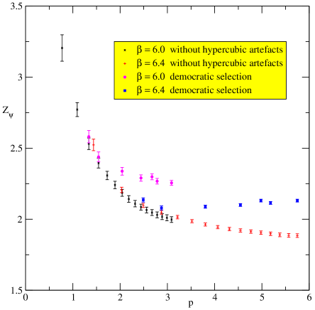
Figure 1: Comparison between the ”democratic” method and our refined treatment for the overlap $Z_{\psi}(p^{2})$ at $6.0$ and $6.4$. Above 2 GeV, precisely where one must study the power corrections, the difference is striking.

4.2.4 The importance of optimising the elimination of hypercubic artefacts

Let us stress then that, as is particularly visible from this comparison, the difference of the $\mathbf{a}^{2}p^{[2n]}$ method with the standard democratic method is not at all academic in the context of the study of power corrections and renormalisation constants. The difference with the previous versions of our method is also not negligible, as we have found.

1) It is obvious that with the standard democratic method, we would obtain quite different results for power corrections and $O(4)$-symmetric artefacts, and therefore for the resulting perturbative contribution. In fact, it has not even been really considered that $Z_{\psi}$ could be affected by such power corrections. 2)Moreover, we observe that the power corrections, as well as the residual $O(4)$ symmetric discretization artefacts, extracted by the previous variants of our method for treating the hypercubic artefacts are not the same ; indeed, when using a previous cruder treatment for overlap action, we have found an important $a^{2}p^{2}$ artefact, which disappears with the more refined treatment, and we were also finding different power corrections (with a weaker condensate). The Wilson case shows similar spuriosities. This means that for a too crude treatment, some hypercubic artefacts can be spuriously mimicked as part of $O(4)$ symmetric discretization artefacts or continuum power corrections. This does not imply that the determination of power corrections is uncertain in this respect, but rather that it is very important to push hypercubic artefact elimination to the best to obtain the genuine continuum power corrections.

Let us finally mention an interesting consequence ; as is well known, the values of Green functions at different momentum points in a Monte-Carlo lattice calculation are highly correlated, which should lead to very small $\chi^{2}/{d.o.f.}$ for fits describing the $p$ dependence by smooth analytic expressions (by small, we mean well below one). It is not found so with too crude treatments of the hypercubic artefacts, because of the erratic oscillations which always remain in the latter methods mimicking statistical deviations. We observe however an impressive decrease of the $\chi^{2}$ down to its expected small value when we improve the treatment of the data, showing that we are now obtaining indeed very smooth functions as physically expected.

5 Proof of the presence of ”non canonical” artefacts : $Z_{V}^{MOM}$ and $O(4)$ symmetric discretization artefacts. Problems for the determination of the continuum limit.

We now start, in the rest of the discussion, from the data obtained through the above treatment of the hypercubic artefacts. They still differ from the continuum by renormalisation and by $O(4)$ symmetric discretization artefacts. It happens that the determination of these artefacts is still harder in general than for hypercubic ones. (as for finite volume artefacts, which we estimate to be weak, see the corresponding short section below).

Indeed, in practice, there is no similar unambiguous method to determine the $O(4)$ symmetric discretization artefacts. True, they manifest themselves by a residual variation with $\beta$, and, in principle, we could study the variation with $\beta$ at each momentum, and then extrapolate to the continuum. However, this requires too many momenta and too much accuracy, if we want really to extract the power correction from the extrapolation to the continuum.

a) a general method for treating $O(4)$ scalar artefacts

Then, a more practical method consists in assuming a prescribed analytical form for both the continuum and the artefacts, with some unknown parameters to be determined by $\chi^{2}$ adjustment.

One has therefore to appeal to our a priori knowledge a) of the continuum, as function of $p$ ; b) of the structure of $O(4)$ symmetric artefacts, as function of $p$ and $a$, so that we could make fits with prescribed functions depending on a limited number of free parameters. For the continuum, this is exactly what is provided by the OPE, with the renormalisation constants $z_{b}$ and $\langle A^{2}\rangle$ as free parameters. For $O(4)$ symmetric artefacts, a standard idea is to recourse to lattice perturbation theory, in which the structure of artefacts is easily explicited. After all, this is what we have invoked for the hypercubic artefacts. As for $O(4)$ symmetric artefacts, the result is quite simple : in the case of a scalar function, and in the chiral limit, where there is no other dimensioned parameters than $a$ and $p$, there can be no other artefacts than $a^{n}p^{n}$, with $n>0$. Then we could work with a few parameters only.

b) why it fails

But now, there appears a very unfortunate circumstance. It is seen that this usual assumption of a perturbative structure of artefacts does not work at all, at least in general. We observe undoubtedly $O(4)$ symmetric artefacts decreasing with p, i.e. for instance of the form $1/p^{n}$ and $n>0$ times some positive power of $a$. To show it, the best way is to consider the $p$ dependence of $Z_{V}^{MOM}=g_{1}/Z_{\psi}$, which should be momentum independent close to the continuum limit. Any $p$ dependence is therefore to be attributed to artefacts. Now, the lattice data show quite clearly a very strong $p$ dependence of $Z_{V}^{MOM}$ except at large $p$. This is true for clover action, and for overlap action as well, see Fig. 2 for overlap fermions.

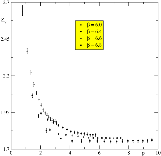
Figure 2: Overlap $Z_{V}^{MOM}$ as function of momentum, respectively for $\beta=6.0$ and $6.4$, and $\beta=6.6$ and $6.8$, for the overlap action. The strong momentum dependence which is displayed must be entirely attributed to artefacts.

The artefacts are similar ; they decrease monotoneously with increasing $p$ for $\beta=6.4,6.6,6.8$; they could be fitted by negative powers of the momentum squared ; for the overlap case, this is also true for $\beta=6.0$ .

c) consequences for determination of power corrections

The necessity of taking into account such negative powers of $p$ is very embarrassing, because, as we explained, we cannot distinguish the $O(4)$ symmetric discretization artefacts by the sole $\beta$ dependence ; we have to rely on the $p$ dependence. Now, it is clear that we will have much difficulty in distinguishing the power corrections and the artefacts decreasing with $p$, and therefore to determinate the condensate. One of the problems is that when increasing the number of negative power terms in the description of the artefact, the tendency is to get alternating signs, and therefore rather unstable results. There is no rationale as to where we should stop. In addition, we must consider that we have also as parameters in the fit the renormalisation constants $z_{b}$, which are practically chosen as an independent parameter at each $\beta$. To add to the uncertainty, we observe that within the precision of the data, we can obtain equivalently good solutions by modifying the $O(4)$ artefacts with a correlative change in the $z_{b}$’s. Then, in spite of many efforts, we have in fact not been able to extract stable and accurate values of $\langle A^{2}\rangle$ by this method, although we have got a clear signal that it is positive and sizable. Then, we have been able to fix the continuum power corrections only by exploiting particular circumstances, to which we devote the rest of the analysis, after a few words on finite volume artefacts.

6 Finite volume artefacts

Let us recall that in the Wilson case [38], we have found only very small volume artefacts, after a careful study with $8^{4},16^{4},24^{4}$ lattices. Only the first points with smallest $n^{2}$ were showing some effect.

We have not performed the same tests for the overlap action, because of the slowness of numerical calculation ; we have only ran on a $16^{4}$ lattice. We are conscious that this is a possible weak point, since this volume is small, and we rely mainly on the analysis of overlap results for the determination of the condensate. So we think of extending this analysis to larger volume as soon as possible.

We stress however that the consistency which is obtained for the continuum power corrections between the overlap results and the S-W (clover) ones with a greater volume $24^{4}$ (see section 9), is a further proof that the volume effects are not crucial for our purpose of determining the condensate.

We must also observe that we can determine the condensate mainly from our large $p$ data ($p>4-5~{}GeV$)(see 7.1), with large $Lp$, where volume artefacts are expected to be even smaller.

6.1 Discretisation or volume artefacts ?

The fact that the above $O(4)$ symmetric artefacts are observed at small $p$ -and only at small $p$ is deserving a special discussion, since it is so counter to usual expectation. Our ears are indeed accustomed to the dictum : ”artefacts at small $p$, finite volume artefacts”, ”artefacts at large $p$, finite spacing artefacts”. Why are they not volume artefacts ? Since it is one important finding of our study, we collect here our arguments.

Let us stress that, in the overlap case, the use of a small volume $16^{4}$ at large $\beta$, to which we are constrained, is not the reason for our finding of large $O(4)$ symmetric artefacts at small $p$. The first argument is that they are also seen in the clover case where we have tested in detail the smallness of volume artefacts; to reiterate, we have seen that only one or two of the smallest momenta seem affected by a volume dependence, while the artefacts we are discussing now are present over a large number of points .

Moreover, let us stress that they have the typical behavior of discretisation artefacts, i.e. they decrease at large $\beta$ and fixed $p$ : indeed, $Z_{V}$ (which should be flat in the continuum limit) is flatter and flatter as $beta$ increases at fixed number of sites $16^{4}$, i.e. as the physical volume decreases. More precisely, we observe that, as the volume decreases, we have more and more points where it is flat, i.e. where it has small artefacts : the respective number of points is $0$ at $\beta=6.0$, $3$ at $\beta=6.4$,$9$ at $\beta=6.6$, $14$ at $\beta=6.8$. This is exactly counter to a volume effect, for which the flatness should be obtained for $n^{2}$ larger that some fixed number. In other terms, for a volume effect, we would expect the artefacts to vanish at smaller and smaller values of $p$ as $\beta$ decreases (i.e. when the physical volume increases). Instead, we find that they vanish around $4-5~{}GeV$ irrespective of $\beta=6.4,6.6,6.8$ ; even more, at $\beta=6.0$, with the largest volume, $Z_{V}$ never becomes flat .

On the other hand, we have no understanding of why $Z_{V}^{MOM}$ seems devoid of sizeable artefacts at large $p$ : it must be regarded as an accident. But it must be underlined that this is not an accident specific to our particular problem. It is a well-known fact, on which any MOM practitioner is relying without being able to explain it : one measures the $Z$’s in regions of large $p$, assuming that artefacts are small, although they would be expected to be large precisely there from lattice perturbation theory.

7 Cases with small $O(4)$ symmetric artefacts with the overlap action at $s=0$. Determination of the condensate.

As we have underlined as conclusion of section 5, paragraph c), the $O(4)$ symmetric artefacts we have found, when present, impede a clear determination of the power correction. It is fortunate that they seem absent or small in some cases. All correspond to overlap action ; then the results are convincingly consistent. Therefore, we concentrate on the overlap fermions in the present and following sections (7,8). As concerns the clover action, we will not be able to have so compelling conclusions, but we show that they are at least compatible (see section 9).

7.1 Large $p$ ($p\sim or>5~{}GeV$)

At this point, we notice that the above difficulties may disappear first at large $p$, above roughly $5~{}GeV$ (therefore at $\beta=6.4,6.6,6.8$), because $Z_{V}$ is constant in this region, especially for the overlap action ; therefore it is suggestive that the artefacts of $Z_{\psi}$ and $g_{1}$ are small there, barring for the unprobable eventuality that $Z_{\psi}$ and $g_{1}$ would happen to have exactly the same artefacts. We then fit $Z_{\psi}$ and $g_{1}$ with a formula containing no $O(4)$ artefact,. i.e. we take only the continuum expression times the renormalisation factor $z_{b}$, at fixed $\beta$, and we obtain then a very encouraging conclusion. Choosing the window of $p$ within which $Z_{V}$ is well constant, we obtain at each $\beta=6.4,6.6,6.8$, and for $Z_{\psi}$ and $g_{1}$, i.e. for six independent data, almost the same condensate value ; we quote a common fit (see the Fig 3) to the three $Z_{\psi}$, with $p_{min}=5,5,4~{}GeV$ respectively, corresponding to the respective $p$ where $Z_{V}$ is beginning to be flat :

$$\langle A^{2}\rangle\simeq(3.1\pm 0.3)~{}GeV^{2}$$ (32)

large and positive, with a rather small error, and quite consistent with what is found in the gluon sector (see below). The $\chi^{2}/d.o.f.=0.07$ is very small as expected from very correlated data. Let us recall that this value of $\langle A^{2}\rangle$ is obtained with the convention that the Wilson coefficient of the operator is expressed in terms of $\alpha_{s}^{MOM}$.

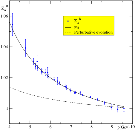
Figure 3: Renormalised overlap $Z_{\psi}$ at $\beta=6.4,6.6,6.8$ and large $p$, compared with the purely perturbative result . The fit of the solid line is made with the perturbative part and only the condensate term , in the windows where the respective $Z_{V}^{MOM}$ become flat (solid line). One finds $\langle A^{2}\rangle=3.1\pm 0.3$. Note that $Z_{\psi}$ is still far from being flat. It has a monotoneous decrease, of around $6\%$ over the range, mainly due to the condensate. The dotted line is the purely perturbative result, clearly inconsistent with the data. Normalisation is made at $10~{}GeV$. $g_{1}$ is described by a similar fit.

A remarkable feature of this region of momentum is that both $Z_{\psi}$ and $g_{1}$, and therefore $Z_{V}$ too, are almost independent of $\beta$. We take it as a further indication that artefacts are accidentally small there.

Let us reinsist that the value of the condensate given in eq. (32) corresponds to the convention, always followed in this paper, that the Wilson coefficient of the operator, calculated only at leading order, is expressed in terms of $\alpha^{MOM}$. The choice of $\alpha^{\overline{MS}}$, would lead to an appreciably higher value (larger by around $70\%$). However, what is important is that the power correction by itself is well determined by our analysis, almost independently of such a change. Indeed, let us replace the OPE expression for the power correction by a simple power, without logarithms corresponding to $\alpha_{s}$, while maintaining the full perturbative expressions for the perturbative part. The fit then gives for the coefficient $c$ of the power term $c/p^{2}$:

$$c=(0.767\pm 0.083)~{}GeV^{2}$$ (33)

when using $\alpha^{MOM}$ in the perturbative part, and :

$$c=(0.844\pm 0.083)~{}GeV^{2}$$ (34)

a small change indeed, of only $10\%$, reflecting the small change of the perturbative part, which is calculated by theory to a great accuracy.

7.2 $Z_{\psi}$ over the whole allowed range of $p$

In addition, we observe another fact : $Z_{\psi}$ - but not $g_{1}$ - is strikingly independent of $\beta$ over the full range of $p$. We have no explanation for that, but we can at least interpret this as meaning that $Z_{\psi}$ is free of $O(4)$-symmetric artefacts over all this range. And indeed, we can fit $Z_{\psi}$ on the full range $p>2.6~{}GeV$ allowed for the perturbative calculation, and the four $\beta$’s with :

$$\langle A^{2}\rangle=(2.73\pm 0.21)~{}GeV^{2}$$ (35)

See the figure 4.

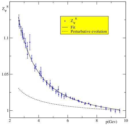
Figure 4: Overlap $Z_{\psi}$ at $\beta=6.0,6.4,6.6,6.8$, renormalised at $10~{}GeV$. The fit for $Z_{\psi}$ extends to the full allowed range of momentum, with $\beta=6.0$ included, and a close value of the condensate $\langle A^{2}\rangle=2.75\pm 0.2$. The dotted line is the purely perturbative result.

We thus obtain a remarkable similarity of the condensate with the previous value. We also obtain similar results by varying the window of the momenta, provided the lower limit is not pushed beyond $5~{}$ GeV, and also by selecting various triplets of $\beta$ values. This seems to support the consistency of our assumptions about artefacts.

If we want to still improve the agreement with the large $p$ analysis, we can introduce a further $1/p^{4}$ term, accounting for the possibility that we may not be sufficiently asymptotic to have a good description with the $1/p^{2}$ condensate alone. For the full window, and the four $\beta$’s, we obtain a very good fit with :

$$\langle A^{2}\rangle=(3.2\pm 0.3)~{}GeV^{2}$$ (36)

and with a small subleading term:

$$(-1.1\pm 0.4)~{}GeV^{4}/p^{4}$$ (37)

with a minus sign which explains that the value of $\langle A^{2}\rangle$ is slightly higher than in the preceding fits. It is then closer to the large $p$ fit.

7.3 $Z_{V}^{MOM}$

From our analysis, we can deduce values of $Z_{V}^{MOM}$ standardly defined, i.e. free from artefacts :

$$Z_{V}^{MOM,~{}large~{}p}(6.4)=1.798\pm 0.012,$$

$$Z_{V}^{MOM,~{}large~{}p}(6.6)=1.776\pm 0.003,~{}~{}Z_{V}^{MOM,~{}large~{}p}(6.8)=1.756\pm 0.011$$ (38)

”$large~{}p$” superscript being to recall that we have selected the value at large p, where we hope to have small $O(4)$ artefacts, in view of the observed flatness ; the precise value is obtained by a fit. For $\beta=6.0$, we quote $Z_{V}^{MOM,~{}large~{}p}(6.0)=1.878\pm 0.014$, but $Z_{V}^{MOM}$ is not yet flat at the highest momentum. Let us repeat that it is remarkable, and perhaps surprising, to observe such a constancy with $\beta$, while one loop perturbation theory would predict a strong variation with $\beta$.

7.4 Comparison with lattice perturbation theory

The fact that $Z_{\psi}$ and $Z_{V}$ are very different from $1$ (in fact not far from $2.$) in the overlap case with $s=0$ may seem surprising. But in fact, already in lattice perturbation theory, the tendency is that the one-loop corrections to $Z_{\psi}$ and $Z_{V}$ are large, because of a very large tadpole contribution to the self energy [31, 29] (while $g_{1}$ remains close to $1$ as we find non pertubatively). The net effect is already large at $\beta=6.0$,for the usual $s=0.4$ : $Z_{V}=1.247$, and still larger for our $s=0$ : $Z_{V}=1.444$ ; we use Table 1 of ref. [29] for the analytical expressions (the definition of $Z_{\psi}$ is different, but by a negligible amount); the numbers are quoted assuming a $BPT$ boosted coupling with $g_{BPT}^{2}=1.68$ (see ref. [31] under eq. (44)). Of course, what is surprising is first that the non perturbative determination (38) is still much larger, and, second, that it is almost independent of $\beta$ over a large range.

Note that the value found by ref. [30] for $Z_{A}$ at $\beta=6.0$,$Z_{A}=1.55$, which should equate $Z_{V}$, is also much larger than BPT ; however, this is not $Z_{A}^{MOM}$ as measured directly ; it is the $Z_{A}$ deduced from hadronic W-T identities. One may think of large artefacts which render different the results from various definitions of $Z_{A},Z_{V}$ ; our study below, section 8.2, shows indeed the presence of such effects, very large at $\beta=6.0$; but they are decreasing rapidly at larger $\beta$, and our finding is that, at $\beta=6.8$, $Z_{V}^{MOM}$ is still much larger than the boosted lattice perturbation theory.

8 $Z_{V}$ and $Z_{A}$. Consistency checks of the overlap action results. Complementary studies on chiral symmetry and artefacts

To ascertain the soundness of our analysis, which may be surprising in several respects, we also perform several consistency checks of general nature in the overlap case ; indeed, some strong statements deriving from chiral symmetry can be formulated.

8.1 $Z_{A}/Z_{V}$ in the non perturbative MOM scheme

One should expect $Z_{A}^{MOM}/Z_{V}^{MOM}$ for the improved Green functions to be exactly 1, i.e. without any artefact in the chiral limit, and in the perturbative regime, i.e at large momentum. This derives from the exact chiral symmetry of the action, discovered by Luescher,combined with the choice of the improved current, or equivalently, of improved Green functions. However, one has also to assume the symmetry of the vacuum state, therefore the absence of spontaneous symmetry breaking. Therefore this result only holds at large momenta. We find indeed this to a high accuracy, fig. 5. Above $2~{}GeV$, for the four $\beta$’s, we have $Z_{A}^{MOM}/Z_{V}^{MOM}=1$ to a very high accuracy. On the other hand, we see that for lower momentum i) the ratio differs from 1, and ii) it depends on $\beta$. The change of regime is rather abrupt. Observation i) has also been made for domain wall fermions at $\beta=6.0$ [41].

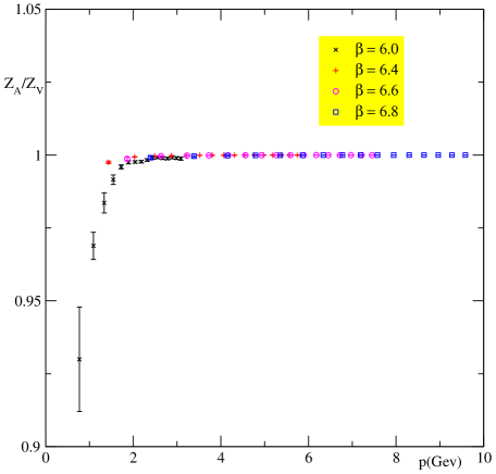
Figure 5: $Z_{A}^{MOM}/Z_{V}^{MOM}$ for overlap fermions and small quark mass at the four $\beta=6.0,6.4,6.6,6.8$. The ratio is 1 above $2~{}GeV$, but differs from 1 and depends on $\beta$ below $2~{}GeV$.

8.2 $Z_{A}$ from a hadronic W-T identity against $Z_{V}^{MOM}$

In principle, once artefacts and power corrections have been eliminated, the various ways of defining the renormalisation constants can be related by perturbation theory. In the case of $Z_{V}$ or similar cases, for the same action, implying identical finite parts, they should even be equal. Moreover, $Z_{A}$ should be equal to $Z_{V}$ from the chiral symmetry of the overlap action.

We verify this statement, as a highly non trivial consistency check of our treatment, by measuring $Z_{A}$ from a standard hadronic Ward-Takayashi identity. $Z_{A}^{WI}=m_{q}/\rho$, where :

$$\rho=1/2<\partial_{0}A_{0},P_{5}>/<P_{5},P_{5}>$$ (39)

In contrast to $Z_{V}^{MOM,large~{}p}$, $Z_{A}^{WI}$ presents a very strong variation with $\beta$ : at $6.0$, the situation seems hopeless, with $Z_{A}^{WI}\sim 3$, but the decrease is rapid :

$$Z_{A}^{WI}(6.0)=3.03,Z_{A}^{WI}(6.4)=2.046,Z_{A}^{WI}(6.6)=1.90,Z_{A}^{WI}(6.8)=1.78$$ (40)

and one reaches finally a level close to $Z_{V}^{MOM,~{}large~{}p}$. Moreover, $Z_{A}^{WI}(a)$ is linear in $a^{2}$ to a very good precision :

$$Z_{A}^{WI}(a)=1.65+5.52a^{2},$$ (41)

which shows that the difference $Z_{A}^{WI}-Z_{V}^{MOM,large~{}p}$ is indeed a discretisation artefact, as it should, and one of the most canonical species, since we expect precisely chiral symmetry breaking to be at most ${\cal O}(a^{2})$. Indeed, on hadron states, the Ward identity is valid up to ${\cal O}(a^{2})$, and Green functions at large $p$, where we measure $Z_{V}^{MOM,large~{}p}$, have also only ${\cal O}(a^{2})$ artefacts from chiral symmetry arguments, in the chiral limit.

9 Check through the Wilson clover $Z_{\psi}$

In view of the rather paradoxical situation which allows us to determine $\langle A^{2}\rangle$ from the $s=0$ overlap action, it is important to reascertain this analysis by a study of the standard clover action, to check whether we can obtain a similar continuum result. Let us stress indeed that from renormalisability, the whole continuum function must be the same up to an overall constant for all the versions of the action. A priori, as we have said, the Wilson case may seem hopeless because there are large $O(4)$ artefacts even in $Z_{\psi}$ ; and even at large $p$, $Z_{V}$ is not so flat

However, one can benefit from the knowledge gained in the overlap case. In the end, the situation appears in fact somewhat similar for the clover action as concerns $O(4)$ symmetric artefacts: the main burden of non canonical artefacts appears to concern $g_{1}$, and we can obtain a good description of $Z_{\psi}$ with a minimal $a^{2}p^{2}$ canonical artefact, and just one $a/p^{2}$ term. Indeed, we obtain :

$$\langle A^{2}\rangle=(2.4\pm 0.3)~{}GeV^{2}$$ (42)

with artefacts

$$-(0.005\pm 0.0015)~{}a^{2}p^{2}-(1.9\pm 0.4)~{}GeV^{3}~{}a/p^{2}$$ (43)

In the present case, the role of these artefacts is crucial to obtain the condensate. In fact, before extraction of these artefacts, the clover data show a rather flat behavior at large $p$, or even an increase at $6.8$. The term with $a/p^{2}$ considerably improves the fit, with a $\chi^{2}$ divided by 3, and brings in a value of the condensate quite close to the one obtained with overlap fermions . These results seem a signal that we have obtained a rather accurate treatment of artefacts. Of course, one may be worried of having introduced a non canonical artefact, which was not necessary in the overlap case ; yet, we must remember that there is no logical reason why such terms should be absent (in the overlap case, they are present anyway in $g_{1}$).

With a subleading term

$$\propto 1/p^{4}$$ (44)

we obtain a still somewhat better agreement with the overlap condensate :

$$\langle A^{2}\rangle=(2.83\pm 0.35)~{}GeV^{2}$$ (45)

The subleading term is also of same sign and comparable magnitude as for overlap action :

$$(-1.85\pm 0.85)~{}GeV^{4}/p^{4}$$ (46)

Note that the consistency of the Wilson $24^{4}$ results with the overlap analysis is comforting the idea that the volume effects are not too important in the overlap case, although certainly they are less compelling because of the need to introduce the $a/p^{2}$ artefact.

10 Consistency with the gluon analysis

To stress the overall consistency of the analysis, one has also to consider the agreement with the previous gluon analysis. We quote the result of a combined fit of $\langle A^{2}\rangle$ and $\Lambda_{QCD}$ to the gluon propagator and the symmetric three-gluon vertex [19] :

$$\langle A^{2}\rangle=(3.6\pm 1.2)~{}GeV^{2}~{}(~{}\alpha_{MOM}~{}),~{}(2.4\pm 0.6)~{}GeV^{2}~{}(~{}\rm{gluon~{}propagator}~{})....$$ (47)

with $\Lambda_{QCD}=0.233\pm 0.028~{}GeV$, and three-loop anomalous dimensions (the use of our present $\Lambda_{QCD}=0.237$ would lower somewhat the condensate values). The fit has been done with the same convention as for quarks, that the Wilson coefficient (calculated only to one loop) is expressed in terms of $\alpha_{s}^{MOM}$. (We could get free from this convention by comparing the magnitude of power corrections themselves as in eq. 33). The coincidence of the values of $\langle A^{2}\rangle$ with the quark value is highly significant since it concerns the continuum function, extracted by a series of various, independent, manipulations committed on the gluon and quark Green functions, and since these continuum functions are related only thanks to the OPE.

The quark measurement has much smaller statistical errors. This is simply due to the fact that in the gluon case, we have left free the value of $\Lambda_{QCD}$, and moreover, the value of the condensate depends strongly on this value, whence the large errors in the gluon case. On the contrary, in the quark case, we have chosen a fixed $\Lambda_{QCD}=0.237~{}GeV$. Indeed, in this case, the dependence on $\Lambda_{QCD}$ is rather weak. Then it is useless to try to determine $\Lambda_{QCD}$ from the fit, and on the other hand the value obtained for $\langle A^{2}\rangle$ remains well determined if we allow some variation in $\Lambda_{QCD}$. Another advantage of quarks is that we can reach the accuracy of four loops in the theoretical expression for the purely perturbative part. In the gluon case, such an accuracy is only possible for the asymmetric vertex, but in that case, the leading term in OPE is not given by $\langle A^{2}\rangle$ [20].

11 Conclusions and discussions

11.1 Physical results and evidences of various artefacts

Let us summarize our results in the following few points :

• First of all, and this is the main point, let us stress that we have finally obtained a rather non trivial confirmation of the validity of the OPE in the non gauge-invariant sector of lattice QCD (treated numerically). The virtue of OPE is that one can describe the departure of all the various Green functions from the perturbative approximation at large momenta with the same set of expectation values. We have now obtained consistency not only between gluon Green functions, but also with the quark sector. This is highly non trivial. Let us recall that there is often some doubt raised about OPE itself, and the possibility is sometimes considered that power corrections could be present not corresponding to an operator v.e.v. The final consistency of the determination of the condensate from three distinct type of Green functions strongly suggests that this is not the case, at least for leading power $1/p^{2}$ corrections. We do identify an OPE power correction, consistently related to $A^{2}$. $\langle A^{2}\rangle$ is found consistently large and positive. The precise magnitude of $\langle A^{2}\rangle$ is affected by an important uncertainty, due to the low accuracy of the theoretical calculation of the Wilson coefficient. But the power correction (i.e. the product of the coefficient and the condensate) is well determined by the lattice analysis, and the ratio of the power corrections in the various Green functions is actually as expected from lowest order OPE.

• It turns out that the lattice discretisation artefacts are unusually sizable in the quark propagator $Z_{\psi}$, but a clearcut distinction must be made between hypercubic artefacts, which are gigantic, but can be efficiently eliminated, and the $O(4)$ symmetric ones, which are not so catastrophic, but that we have not been able to handle systematically.

• We believe that we have been really efficient in getting rid of the hypercubic artefacts thanks to our (improved) method of ”restoration of $O(4)$ symmetry”.

• Once these artefacts have been subtracted, the overlap $Z_{V}(p^{2})\equiv Z_{\psi}(p^{2})/g_{1}(p^{2})$, which should be independent of $p$ except for artefacts, is very close to a constant at large $p>5~{}GeV$. This is far from trivial and supports the statement that we have no remaining $O(4)$ symmetric artefacts in this specific region. This is directly supported by the near constancy of the quantities as function of $\beta$.

  Moreover, also in the overlap case, but for $Z_{\psi}(p^{2})$ only, the same statement of constancy with $\beta$ extends down to the lowest momenta ; this leads to suspect that $O(4)$ symmetric artefacts are small in this case over the whole range of $p$. We are unable to explain these two special situations .

  Let us recall that a certain flatness $Z_{V}(p^{2})$ at large $p$ is also observed with the Wilson quark action, although it is not so good. Let us recall also that this region is the basis for the standard determinations of MOM renormalisation constants, usually with the Wilson quark action (see for example [42], which presumes that discretisation artefacts are not large there. Let us then recall that we have no theoretical argument supporting the statement that they are not large. Quite the contrary. If any, the theoretical arguments would suggest them to increase with $p$. The support is purely empirical. This is embarrassing if we aim at precision determinations.

• $Z_{V}$ of the overlap action at $s=0$ is large, around $1.8$, in qualitative agreement with BPT perturbation theory which finds large self-energy contributions in $Z_{\psi}(p)$. But it is still much larger than the expectation, and the lack of dependence on $\beta$ is not understood from perturbation theory.

• Considering the cases where the $O(4)-symmetric$ artefact-free results are supected to be small, we try to fit them by OPE, i.e. by the four-loops perturbative contribution plus the $<A^{2}>$ condensate contribution computed to leading logarithm. The overlap $Z_{\psi}$ and $g_{1}$ at large $p>5~{}GeV$ allow for a good fit for $\beta=6.4,6.6,6.8$, leading to a consistent $<A^{2}>$ not far from $3~{}GeV^{2}$. The overlap $Z_{\psi}$ also allow for a good fit for the whole range $p>2.6$ GeV , including in addition $\beta=6.0$. The $<A^{2}>$ condensate is consistent with the former value. A very small $1/p^{4}$ term still improves the consistency.

• In the other cases, namely in $g_{1}$ and $Z_{V}$ for $p$ lower than $p\sim 5~{}GeV$, the $O(4)-symmetric$ artefacts become large, especially at small $p$, and in fact, they increase regularly from large to small $p$. This trend, which is also contrary to the expectation of lattice perturbation theory, clearly indicates a non perturbative origin. In fact, one important conclusion of our study is the existence of these very large non perturbative artefacts at small $p$ due to discretisation. These are very embarrassing for any analysis of the Green functions, as we comment below.

  Let us repeat our strong conviction that these low $p$ effects(under $2~{}GeV$) are indeed discretisation artefacts and not volume artefacts. They behave quite counter to volume effects, as we have extensively argued.

• A short study of $Z_{A}^{MOM}/Z_{V}^{MOM}$ shows that similar artefacts are still present in a ratio where they would be expected to cancel if one applies naively the exact chiral symmetry of the lattice action. They are clearly seen as being discretisation artefacts because they are reduced at larger $\beta$. They seem to be present on top of an actual continuum effect, small but visible, which could be due to continuum chiral symmetry spontaneous breaking. One can suspect that the artefacts themselves are connected with the spontaneous breaking of chiral symmetry.

  It seems logical that such chiral-symmetry violating artefacts, as well as the continuum effect, be only forbidden at large $p$, if they are connected with spontaneous breaking effects. Indeed, it is there and only there that such effects fade away. Therefore, it is consistent with this interpretation that we find $Z_{A}^{MOM}/Z_{V}^{MOM}=1$ at large $p$ to a high precision, without $\beta$ dependence.

• Of course, the clover (SW) action has the great advantage that it does not present the same very constraining limit in volume as the overlap one ; however, it leads to less compelling results than the overlap one, because we have not found here the same particular situations where $O(4)$ artefacts can be neglected ; the small $p$ artefacts, which render so difficult the determination of power corrections, are present in $Z_{\psi}$ and not only in $g_{1}$. As explained above, by including more and more terms to describe these artefacts, we destabilize the numerical value of $\langle A^{2}\rangle$. Stopping with the first term $a/p^{2}$, we obtain consistency with the overlap results.

• As to comparison with other works on the quark propagator, the question of the presence and magnitude of power corrections is a crucial test of the precision obtained in the treatment of Green functions : the condensate value $\langle A^{2}\rangle$ should be independent of the action and of $\beta$ with due renormalisation. In our opinion, safe and accurate extraction of power corrections requires a very large range of momenta, and therefore a large range of $\beta$ ; indeed, to use a rather large range of momenta at a fixed $\beta$ would be dangerous because of the periodicity of the lattice ; the large $p$ behavior would then be highly dependent on empirical redefinitions of the momenta, aiming to remove empirically lattice artefacts at very large $p\simeq 10~{}GeV$. Of course, a crucial question is whether one can work with a $\beta$ as large as $6.8$ with our lattice size $16^{4}$- the possible size is indeed strongly restricted for the overlap action. It is our conviction, for reasons which have been explained in detail. Another concern is that, according to our experience, to extract the real power corrections, one needs a particularly careful elimination of hypercubic artefacts.

• The resulting value of $\langle A^{2}\rangle$ from the OPE analysis of lattice QCD data should be compared to tentative estimates made by various authors within analytical approaches. One will find abundant references in the paper of Dudal et al., ref. [43]. It is clear that this comparison must take care of the precise definition of the condensate, as regards for instance renormalisation.

11.2 Systematic errors on $\langle A^{2}\rangle$

Of course, we are making many assumptions which introduce uncertainty in the value of $\langle A^{2}\rangle$. Recall that we do not claim to determinate it only from the present study, since we have several previous determinations from the gluonic sector. So we can also appreciate systematic errors from the consistency we obtain with these previous estimates (see above, section 10). In fact, as we have observed in section 10, the gluon propagator determination and the one from $\alpha_{s}$ are notably different, but the values are affected by very large errors, and are compatible with the present ones. From all the determinations, we could conclude that the systematic errors do no seem to exceed $1~{}GeV^{2}$. But there is in fact an important source of systematic error, which is explained below, and which cannot be estimated by comparison with gluons because it is present in both: it is the fact that the Wilson coefficient is calculated only at low order. Then, it remains useful to discuss the sources of errors inside the quark sector itself, for which anyway the conditions are intrinsically very favourable.

Since we do not claim to do phenomenology, but rather an exercise in quenched QCD, we have not to bother about the quenched approximation, which is also supposed for gluons. Chiral limit is assumed on the theoretical side, for instance to calculate the Wilson coefficents. Now, of course, we do not work at zero quark mass on the lattice. We have not tried to do a systematic chiral extrapolation on the lattice data, which would only lead to increase the statistical errors. We observe that $Z_{\psi}$ seems very weakly dependent on our set of masses, which means that this limit is not a priori a problem at the smallest mass (at which we have made all our OPE analysis). Anyway, we can discard any catastrophic effect at very low quark masses through the consistency with the quenched gluon data.

Let us now pass to more relevant effects.

Some come from the treatment of artefacts, for which we lack of theoretical basis, some are relative to our description of the continuum, which, although based on a much stronger theoretical basis, involves necessarily approximations.

We do not return to finite volume artefacts, since we have nothing quantitative to say about their magnitude in the overlap case. For what concerns hypercubic artefacts, we may have an idea on the error remaining in their treatment by the variation observed with two variants, with a slightly different description of the continuum limit :

$$\langle A^{2}\rangle=(3.23-3.0)~{}GeV^{2}$$ (48)

Whenever large $O(4)$ symmetric artefacts are present, we are compelled, as we have seen, to rather arbitrary assumptions on their structure, since we have concluded that we cannot rely on lattice perturbation theory. The correlated errors in our determination of the ”non perturbative” artefacts and of the condensate seem very large, as judged from the range of values obtained in various fits, to such a point that we have renounced to extract any number in this case. Therefore, we consider only the case where we have strong hints that the artefacts are small, in which case we have mainly to consider uncertainties in the continuum description. They are themselves of two origins : the perturbative calculation of Wilson coefficients ; the non perturbative aspect, i.e. the relevance of the OPE expansion, the enumeration of operators… As to uncertainties in perturbative calculations :

i) We have checked that computing the perturbative contribution to third or fourth order in perturbation does not change significantly the estimated condensate (only $7\%$ of change). Another test is to reexpress the series in terms of $\alpha_{\overline{\rm MS}}$ instead of $\alpha_{\rm MOM}$. $Z_{\psi}$ changes by less than $1\%$ with various prescriptions. We can thus assume that the perturbative contribution has been expanded far enough.

ii) As we have explained in subsection 2.3, the problem is much more important for the Wilson coefficient of the $A^{2}$ operator which has, on the contrary, only been computed to leading logarithm. A sign of this problem is seen by changing $\alpha_{\rm MOM}$ into $\alpha_{\overline{\rm MS}}$. A change of $\alpha_{\rm MOM}$ into $\alpha_{\overline{\rm MS}}$ reduces it by fourty percent $\alpha_{s}(10{\rm GeV})$, and more for the smaller momenta; whence a reduction of the Wilson coefficient by $50\%$ in average. Through a conspiracy with the smaller change in the perturbative contribution, this change amounts to an increase of the resulting condensate by $70\%$. Of course, similar effects are present for gluons, and, as we have explained, the ratio of condensates obtained from quarks and gluons will remain the same. More importantly, one must be aware that the power correction by itself remains well determined; what is not well determined is the translation of the power correction into a $\langle A^{2}\rangle$ condensate value. Indeed, this translation depends on the theoretical evaluation of the Wilson coefficient, which is not accurate at present.

As to the properly non perturbative aspect, we may think of two sources of uncertainties in determining $\langle A^{2}\rangle$. The one stems from other operators which could enter with the same power in the OPE expansion. However, we do not find any such operator contribution in $Z_{\psi}$ in the chiral limit. We could have some contamination since we are not exactly in the chiral limit, but it must be small, since we observe a very weak quark mass dependence. The other could be the possibility that $p$ is not sufficiently large for the leading correction $1/p^{2}$ to completely dominate over next ones. This possibility is represented by the $1/p^{4}$ term and the fact that it is small but non zero in the fits shows indeed that we are not completely asymptotic at such large momenta ; although it is very small, around $1\%$ at $3~{}GeV$, it leads to a change of around $15\%$ in $\langle A^{2}\rangle$. On the other hand, with this term included, we find a very good stability of $\langle A^{2}\rangle$ over the large range $2.6~{}GeV<p<10~{}GeV$, when varying the fitting window, which suggests that we have correctly accounted for the small subasymptotic effects. Actually, this term could also mimick a neglected logarithmic dependence ; indeed, passing from $\alpha^{MOM}$ to $\alpha^{\overline{MS}}$ as expansion parameter as explained above, the $1/p^{4}$ term passes from $-1.1/p^{4}~{}GeV^{4}$ to $-(0.65\pm 0.34)~{}GeV^{4}/p^{4}$, therefore there is an appreciable variation, although the sign and order of magnitude are encouragingly stable.

On the whole, the dependence of the Wilson coefficient on the scheme for $\alpha_{s}$ seems the most worrying source of uncertainty, yet it can be solved soon.

Another concern is the value used for $\Lambda_{QCD}$. Let us vary by $\pm 10\%$ our $\Lambda_{\overline{MS}}=0.237~{}GeV$. We find :

$$\Lambda_{\overline{MS}}=0.215-0.260~{}GeV~{}\to~{}\langle A^{2}\rangle=3.45-3.02~{}GeV^{2},$$ (49)

a quite moderate change indeed. There is naturally an increase for decreasing $\Lambda_{QCD}$ because the larger power correction compensates for the slower falloff of the perturbative part.

11.3 General consequences for lattice studies induced by the observed discretisation artefacts and power corrections. Accuracy on Green functions. Renormalisation in the MOM approach

True, the direct object of this study has been to verify the consistency of our OPE analysis of lattice data by extending it to the quark sector, and then comparing with the previous analysis of the gluon sector; and thereby to assess the soundness of our statement of large power corrections in ”elementary” Green functions as well as of their interpretation in terms of the non gauge-invariant condensate $<A^{2}>$.

However, one must be aware of the strong consequences of this study, as well as of the preceding ones, on general problems, especially in precision studies :

-1) Power corrections. First, we have a problem independent of the discretisation of the action : the presence of the power corrections has the effect of modifying the estimate of quantities defined in the perturbative regime of QCD, when one attempts to extract them from the numerical measures done on the lattice. Indeed, such power corrections, of non perturbative origin, must be necessarily subtracted from the Green functions to get the perturbative contribution, the only one which presents a universal character since it can be translated from one renormalisation scheme to another.

In the gluonic sector, the perturbative contribution leads to a determination of $\Lambda_{QCD}$ ; the necessary extraction of the $1/p^{2}$ power correction induces a striking modification in the value of $\Lambda_{QCD}$, as was found some years ago [17]. Of course, this very large change of $\Lambda_{QCD}$ corresponds to much more moderate corrections on the Green functions themselves, yet they may amount to several percents ($10\%$ at low points).

Now, let us recall that for renormalisation constants of the quark sector, one is also most often looking for the ones defined in the perturbative regime. Indeed, only such perturbative renormalisation schemes can be connected between one another by analytical calculations, and also connected to Wilson coefficients in order to produce physical quantities. But we predict from OPE, and we have indeed observed in this article, that power corrections of the same magnitude affect the quark sector, in particular $Z_{\psi}$ and various vertex functions. From the Ward identity, it happens that for quantities like $Z_{V}$, the $A^{2}$ power corrections cancel between the vertex function and $Z_{\psi}$. But this is not true in general : in $Z_{S}$ and $Z_{P}$ for instance, this cancellation does not occur. In such cases, the power corrections must be subtracted, in principle. Of course, one may wonder whether this is practically important. It depends on the accuracy we want to obtain. If we aim at a precision of a few percent, certainly we do require to take them into account, since they reach several percent around $4~{}GeV$, $5\%$ on $Z_{\psi}$ in the Wilson case. Now, one often claims to go below $10\,\%$ with dynamical quarks ; then,such effects are deserving of consideration.

What simplifies somewhat the problem raised by power corrections is that not only they are independent of the chosen discretisation of the action, but they are often related to the same $\langle A^{2}\rangle$ condensate, at least as regards the dominant power. Once $\langle A^{2}\rangle$ has been confidently determined by one analysis, it can be used in others, the respective contribution to the various Green functions being obtained through the lowest order Wilson coefficients of the OPE.

-2) the $O(4)$-invariant discretisation artefacts that we have found set a more general difficulty, and one which is more embarrassing, in view of our lack of theoretical control. We have no reason to suppose that the special case we have studied is especially catastrophic. Yet, it shows already an embarrassing situation.

$\alpha$-The first step is to have control on hypercubic artefacts to a good accuracy. It is deserving of mention that this accuracy cannot be obtained by the standard method of selecting democratic points. Moreover, the simplest versions of our alternative method of ”restoration of $O(4)$ symmetry” have not allowed to get a good accuracy. We have had to go further. This requires already a good deal of work. But, finally, it seems that we are able to produce a systematic and accurate procedure.

$\beta$-On the other hand, we have not obtained a safe a systematic general method to extract the $O(4)$-invariant artefacts while we have a clear proof that they are large at small $p$. This is disastrous for the extraction of the power corrections. This fact seems to be a problem specific to the quark sector : we had not found similar evidence for gluonic Green functions, although we cannot exclude totally their presence. We have not any theoretical mastering about their magnitude. It is our impression that the perturbation theory is of no help, since they happen in fact to be large at small $p$, and small at large $p$, counter to the expectation of perturbation theory. There is no explanation for the relative flatness of $Z_{V}$ we observe at large $p$, and which is the basis of most determinations of renormalisation constants. Note that this lack of explanation is a problem not only for us, but for all the $MOM$ determinations of renormalisation constants.

One may wonder whether the choice of the quark action may help. The use of overlap action seems to introduce larger hypercubic artefacts, but this is not a decisive obstacle, as we have explained. On the other hand, the fact that in certain cases it presents small $O(4)$-invariant artefacts seems an important advantage. Yet, it is weakened by our lack of understanding of the underlying reasons why it is so. Calculations with other values of $\rho=1+s$ may reveal instructive.

Taking into account these uncertainties coming from $O(4)$-invariant artefacts, which have appeared negligible only for $Z_{\psi}$ and only in the overlap case, but not at all for $Z_{V}$, it is possible that the MOM scheme may reveal not very practicable for precision calculations, although it is appealing by its simplicity, and quite efficient for ordinary purposes. Of course, at this point, one may think of the method of the ALPHA collaboration as a complementary one, technically difficult, but which allows a very clean treatment of discretisation artefacts by using on-shell quantities, and also allows to work at very high energy scale, therefore eliminating power corrections (see for example, for $Z_{V}$, [44]).

12 Acknowledgement

We thank Michele Pepe, Damir Becirevic, Claude Roiesnel. for precious discussions and comments, and M. Pepe for help when initiating this work. Alain Le Yaouanc would like to thank J.-R. Cudell and C. Pittori for many very useful discussions in a previous collaboration on the quark propagator. This work has been supported in part by the European Network “Hadron Phenomenology from Lattice QCD”, HPRN-CT-2000-00145. We have used for this work the APE1000 hosted by the Centre de Ressources Informatiques (Paris-Sud, Orsay) and purchased thanks to a funding from the Ministère de l’Education Nationale and the CNRS.

Appendix A Perturbative expansion to four loops in the full MOM scheme

Our aim is to express $Z_{\psi}(p^{2})$, in terms of $\alpha_{s}^{MOM}$, defined by the triple gluon vertex at symmetric momenta. More precisely, we are looking for the renormalisation group improved expression, which resums the large logs $\log(p^{2}/\mu^{2})$ at large $p$. The expression then takes the form of a series in $\alpha_{s}^{MOM}(p)$ with pure number coefficients. This series can be obtained from the knowledge of the anomalous dimension of $Z_{\psi}$ in terms of $\alpha_{s}^{MOM}$, and of the $\beta$ function of the MOM scheme. This is possible in the Landau gauge to the order of four loops included, thanks to the papers of Chetyrkin and collaborators, ref. [25] and [26].

First, one has in section 4.2 of the first paper the expansion of $\frac{\partial lnZ_{\psi}(\mu^{2})}{\partial ln\mu^{2}}$ as a series in $\alpha_{s}$ of the $\overline{\rm{MS}}$ scheme to four loops (in fact the authors consider the inverse $Z_{2}(\mu^{2})=(Z_{\psi}(\mu^{2}))^{-1}$, so we have to invert their formula). Since there is no $\alpha_{s}$ term in the Landau gauge, to reexpress the series in terms of the $\alpha_{s}$ of the ${\rm MOM}$ scheme at four loops requires the expansion of $\alpha_{s}^{\overline{\rm MS}}$ in terms of $\alpha_{s}^{\rm MOM}$ only to order three included. This expansion is provided by the section 5 of the second paper, by inverting the first equation of this section. On the other hand, we need the MOM $\beta$ function. It is given in the second paper, section 6, at three loops, which is also sufficient to calculate the renormalisation improved series for $Z_{\psi}(p^{2})$ at four loops included ; indeed, the four loop coefficient of the $\beta$ function enters only as a factor of the one loop anomalous dimension of the fermion $\gamma_{0}$ , which is zero in the Landau gauge. We then obtain the following expansions :

-$Z_{\psi}$ is expressed in general as :

$$Z_{\psi}^{pert} = \alpha^{\frac{\gamma_{0}}{\beta_{0}}}\Bigg{(}1+\alpha\frac{\beta_{0}\gamma_{1}-2\beta_{1}\gamma_{0}}{4\pi\beta_{0}^{2}}\quad\quad\quad\quad\quad$$ (50)

$$+ 0.5\alpha^{2}\left(\frac{(\beta_{0}\gamma_{1}-2\beta_{1}\gamma_{0})^{2}}{16\beta_{0}^{4}\pi^{2}}+\frac{8\beta_{1}^{2}\gamma_{0}-\beta_{0}\beta_{2}\gamma_{0}-4\beta_{0}\beta_{1}\gamma_{1}+2\beta_{0}^{2}\gamma_{2}}{32\beta_{0}^{3}\pi^{2}}\right)$$

$$+ \frac{\alpha^{3}}{768\beta_{0}^{6}\pi^{3}}\Big{(}-16\beta_{1}^{3}\gamma_{0}^{3}+24\beta_{0}\beta_{1}^{2}\gamma_{0}^{2}(-2\beta_{1}+\gamma_{1})$$

$$+ 2\beta_{0}^{2}\beta_{1}\gamma_{0}(-16\beta_{1}^{2}+3\beta_{2}\gamma_{0}+24\beta_{1}\gamma_{1}-6\gamma_{1}^{2})$$

$$- 2\beta_{0}^{4}(2\beta_{3}\gamma_{0}+\beta_{2}\gamma_{1}+4\beta_{1}\gamma_{2}-3\gamma_{1}\gamma_{2})$$

$$+ \beta_{0}^{3}\left(16\beta_{1}^{2}\gamma_{1}-3\beta_{2}\gamma_{0}\gamma_{1}+2\gamma_{1}^{3}+4\beta_{1}\left(2\beta_{2}\gamma_{0}-3(\gamma_{1}^{2}+\gamma_{0}\gamma_{2})\right)\right)+4\beta_{0}^{5}\gamma_{3}\Big{)}\Bigg{)}$$

-For $n_{\rm f}=0$ in the Landau gauge, we get :

$$\gamma_{0} = 0.0\quad\gamma_{1}=\frac{67}{3}\quad\gamma_{2}=-94.7943$$

$$\gamma_{3} = 14503.7$$ (51)

-$\alpha$ , which represents here $\alpha_{{\rm MOM}}(p)$ (defined through the three-gluon vertex at symmetric momenta), is given, under the same conditions, by :

$$\alpha(p) = \frac{4\pi}{\beta_{0}\,t}-8\pi\frac{\beta_{1}}{\beta_{0}}\frac{\ln t}{(\beta_{0}t)^{2}}+\frac{1}{(\beta_{0}t)^{3}}\left(2\pi\frac{\beta_{2}}{\beta_{0}}+16\pi\frac{\beta_{1}^{2}}{\beta_{0}^{2}}\left((\ln t)^{2}-\ln t-1\right)\right)$$

$$+ \frac{1}{(\beta_{0}t)^{4}}\left(-32\pi\frac{\beta_{1}^{3}}{\beta_{0}^{3}}(\ln t)^{3}+80\pi\frac{\beta_{1}^{3}}{\beta_{0}^{3}}(\ln t)^{2}\right.$$

$$- \left.\frac{12\pi\beta_{0}\beta_{1}\beta_{2}-64\pi\beta_{1}^{3}}{\beta_{0}^{3}}\ln t+\frac{2\pi\beta_{0}^{2}\beta_{3}-16\pi\beta_{1}^{3}}{\beta_{0}^{3}}\right)$$

where $t=\ln(p^{2}/\Lambda_{{\rm MOM}}^{2})$ (in the MOM case, one stops at the $1/t^{3}$ terms. and where

$$\beta_{0}=11\quad\beta_{1}=51\quad\beta_{2}=3072~{}(10\%)$$ (53)

Appendix B $A^{2}$ Wilson coefficient in the quark propagator

In order to renormalise the bare quark propagator in Eq. (15) we will define the following two renormalisation constants, both in the momentum subtraction (MOM) general scheme :

$$\left(\begin{array}[]{l}Z_{\psi}(\mu^{2})\\ \\ Z^{\rm pert}_{\psi}(\mu^{2})\end{array}\right)\ \delta_{a,b}\ =\ \frac{-ip\!\!\!/+m(p^{2})}{p^{2}+m(p^{2})}\ \left(\begin{array}[]{l}S^{-1}(p)\\ \\ S^{-1}_{\rm pert}(p)\end{array}\right)_{p^{2}=\mu^{2}}$$ (60)

The constant in the top of the l.h.s of Eq. (60) includes the non-perturbative contributions to the quark propagator to let it take the tree-level value all over the energy range (not only in the perturbative regime). We renormalise Eq. (15) by multiplying by that of the bottom (this purely perturbative MOM renormalisation constant, computed to four loops in ref. [25], is presented in the appendix A) ; as to the Wilson coefficient of $A^{2}$, we calculate it at leading RG order.

$$\left(Z^{\rm pert}_{\psi}(\mu^{2})\right)^{-1}\ S^{-1}(p)\ =\ ip\!\!\!/\ \delta_{a,b}\frac{Z_{\psi}(p^{2})}{Z_{\psi}^{pert}(\mu^{2})}+\cdots$$

$$=\ \left(Z^{\rm pert}_{\psi}(\mu^{2})\right)^{-1}\ S^{-1}_{\rm pert}(p)+ip\!\!\!/\ \frac{d\left(\frac{p^{2}}{\mu^{2}},\alpha(\mu)\right)}{p^{2}}\frac{<(A^{2})_{\rm R}(\mu)>}{4(N_{C}^{2}-1)}\ \delta_{a,b}+\cdots$$

$$=\ ip\!\!\!/\ \delta_{a,b}\ \left(\frac{Z_{\psi}^{pert}(p^{2})}{Z_{\psi}^{pert}(\mu^{2})}+\frac{d\left(\frac{p^{2}}{\mu^{2}},\alpha(\mu)\right)}{p^{2}}\frac{<(A^{2})_{\rm R}(\mu)>}{4(N_{C}^{2}-1)}\right)\ +\cdots$$ (61)

where $(A^{2})_{\rm R}(\mu^{2})=Z_{A^{2}}^{-1}(\mu^{2}):A^{2}_{\rm bare}:$ , and where we only write the leading terms in $p\!\!\!/$. Concerning $d\left(\frac{p^{2}}{\mu^{2}},\alpha(\mu)\right)$, the same procedure used for gluon Green functions in refs.[18, 19, 20] is in order here. Then, from Eq. (B), multiplying by $Z^{\rm pert}_{\psi}(\mu^{2})$, and taking logarithm derivatives on $\mu$ in both sides, we obtain the following RG equation:

$$\left\{-\gamma_{0}\frac{\alpha(\mu)}{4\pi}+\gamma_{A^{2}}^{(0)}\frac{\alpha(\mu)}{4\pi}+\frac{d}{d\ln{\mu^{2}}}\right\}d\left(\frac{p^{2}}{\mu^{2}},\alpha(\mu)\right)\ =\ 0$$ (62)

that is identically satisfied with :

$$d\left(\frac{p^{2}}{\mu^{2}},\alpha(\mu)\right)\ =\ d\left(1,\alpha(p)\right)\ \left(\frac{\alpha(\mu)}{\alpha(p)}\right)^{\frac{-\gamma_{F}^{(0)}+\gamma_{A^{2}}^{(0)}}{\beta_{0}}}\ ,$$ (63)

where $d(\left(1,\alpha(p)\right))$ is in fact beginning with $\alpha(p)$ and $\gamma_{A^{2}}^{(0)}$ is defined through :

$$\frac{d}{d\ln{\mu^{2}}}\ln{Z_{A^{2}}}\ =\ -\gamma_{A^{2}}^{(0)}\frac{\alpha(\mu)}{4\pi}+{\cal O}\left(\alpha^{2}\right)\ ;$$ (64)

and where all the involved one-loop coefficients are well known:

$$\gamma_{A^{2}}^{(0)}=\frac{35N_{c}}{12}\ ,\ \ \ \gamma_{0}=0\ ,\ \ \ \beta_{0}=11\ .$$ (65)

On the other hand, $d\left(1,\alpha(p)\right)$ can be obtained by computing the only diagram involved in the “OPE business” for this case,

0.6

$$\ \ \ \ \ \ \ \ \ \ \ \ \ \ \ \ \ \ \ \ \ \ \ \ \to\ \ \ \ \ d\left(1,\alpha(p)\right)=\frac{(N_{C}^{2}-1)}{3}g^{2}(p)$$ (66)

Then, by applying the results from Eqs. (63-65) to Eq. (B), we will obtain the final result Eq. (16) to be used for the fits.

References

- [1] K. D. Lane, Phys. Rev. D 10 (1974) 2605.
- [2] H. Pagels, Phys. Rev. D 19 (1979) 3080.
- [3] H. D. Politzer, Nucl. Phys. B117 (1976) 397.
- [4] M. Lavelle, M. Oleszczuk, Mod.Phys.Lett.A7:3617-3630,1992.
- [5] C. Bernard, D. Murphy, A. Soni, K. Yee, Nucl. Phys. B (Proc. Suppl.) 17 (1990) 593.
- [6] G. Martinelli, C. Pittori, Christopher T. Sachrajda, M.Testa, A. Vladikas,Nucl.Phys.B445:81-108,1995 e-Print Archive: hep-lat/9411010
- [7] D. Becirevic, V. Gimenez, V. Lubicz, G. Martinelli, Phys.Rev.D61:114507,2000, e-Print Archive: hep-lat/9909082
- [8] C. Dawson (Brookhaven) et al., Nucl.Phys.Proc.Suppl.83:854-856,2000 e-Print Archive: hep-lat/9909107
- [9] J. Skullerud, D. B. Leinweber and A. G. Williams, Phys. Rev. D 64, 074508 (2001) [arXiv:hep-lat/0102013]; J. I. Skullerud and A. G. Williams, Phys. Rev. D 63, 054508 (2001) [arXiv:hep-lat/0007028]; J. I. Skullerud and A. G. Williams, Nucl. Phys. Proc. Suppl. 83, 209 (2000) [arXiv:hep-lat/9909142].
- [10] P. O. Bowman, U. M. Heller, D. B. Leinweber and A. G. Williams, [arXiv:hep-lat/0209129].
- [11] J. Zhang, P.O. Bowman, D.B. Leinweber, A.G. Williams, F.D.R.Bonnet, Phys.Rev. D70:034505,2004 [arXiv:hep-lat/0301018]
- [12] T. Bhattacharya, R. Gupta, W. Lee, Nucl.Phys.Proc.Suppl.106:786-788,2002 e-Print Archive: hep-lat/0111002
- [13] J. R. Cudell, A. Le Yaouanc and C. Pittori, Phys. Lett. B 454, 105 (1999) [arXiv:hep-lat/9810058].
- [14] J. R. Cudell, A. Le Yaouanc and C. Pittori, Nucl. Phys. Proc. Suppl. 83, 890 (2000) [arXiv:hep-lat/9909086].
- [15] J. R. Cudell, A. Le Yaouanc and C. Pittori, Phys. Lett. B 516, 92 (2001) [arXiv:hep-lat/0101009].
- [16] D. Becirevic, V. Lubicz, Phys.Lett.B600:83-90,2004 e-Print Archive: hep-ph/0403044
- [17] P. Boucaud et al., JHEP 0004, 006 (2000) [arXiv:hep-ph/0003020].
- [18] P. Boucaud, A. Le Yaouanc, J. P. Leroy, J. Micheli, O. Pene and J. Rodriguez-Quintero, Phys. Lett. B 493, 315 (2000) [arXiv:hep-ph/0008043].
- [19] P. Boucaud, A. Le Yaouanc, J. P. Leroy, J. Micheli, O. Pene and J. Rodriguez-Quintero, Phys. Rev. D 63, 114003 (2001) [arXiv:hep-ph/0101302].
- [20] F. De Soto and J. Rodriguez-Quintero, Phys. Rev. D 64, 114003 (2001) [arXiv:hep-ph/0105063].
- [21] P. Boucaud, J. P. Leroy, J. Micheli, O. Pene and C. Roiesnel, JHEP 9810, 017 (1998) [arXiv:hep-ph/9810322]. D. Becirevic, P. Boucaud, J. P. Leroy, J. Micheli, O. Pene, J. Rodriguez-Quintero and C. Roiesnel, Phys. Rev. D 60, 094509 (1999) [arXiv:hep-ph/9903364].
- [22] D. Becirevic, P. Boucaud, J. P. Leroy, J. Micheli, O. Pene, J. Rodriguez-Quintero and C. Roiesnel, Phys. Rev. D 61, 114508 (2000) [arXiv:hep-ph/9910204].
- [23] P. Boucaud et al., Talk given at 37th Rencontres de Moriond on QCD and Hadronic Interactions, Les Arcs, France, 16-23 Mar 2002. arXiv:hep-ph/0205187.
- [24] D. Becirevic, V. Lubicz, G. Martinelli and M. Testa, Nucl. Phys. Proc. Suppl. 83, 863 (2000) [arXiv:hep-lat/9909039].
- [25] K. G. Chetyrkin and A. Retey, Nucl. Phys. B 583, 3 (2000) [arXiv:hep-ph/9910332].
- [26] K.G. Chetyrkin, T. Seidensticker, Phys.Lett.B495:74-80,2000 e-Print Archive: hep-ph/0008094
- [27] D. Dudal, H. Verschelde, V.E.R. Lemes, M.S. Sarandy, R.F. Sobreiro, S.P. Sorella, J.A. Gracey, Phys.Lett.B574:325-331,2003 e-Print Archive: hep-th/0308181
- [28] ALPHA Collaboration (Stefano Capitani et al.), Nucl.Phys.B544:669-698,1999 e-Print Archive: hep-lat/9810063
- [29] S. Capitani, L.Giusti , Phys.Rev.D62:114506,2000 e-Print Archive: hep-lat/0007011
- [30] L. Giusti, C. Hoelbling, C. Rebbi, Nucl.Phys.Proc.Suppl.106:739-747,2002, e-Print Archive: hep-lat/0110184
- [31] C. Alexandrou, E. Follana, H. Panagopoulos, E. Vicari, Nucl.Phys.B580:394-406,2000 e-Print Archive: hep-lat/0002010
- [32] M. Luscher, S. Sint, R. Sommer, P. Weisz and U. Wolff, Nucl. Phys. B 491, 323 (1997) [arXiv:hep-lat/9609035].
- [33] H. Neuberger, Phys.Lett.B417:141-144 (1998) e-Print Archive: hep-lat/9707022
- [34] P. Hernandez, K. Jansen, M. Luscher, Nucl.Phys.B552:363-378,1999 e-Print Archive: hep-lat/9808010
- [35] S. Capitani, M. Gockeler, R. Horsley, P.E.L. Rakow, G. Schierholz, Phys.Lett.B468:150-160,1999 e-Print Archive: hep-lat/9908029
- [36] Stefano Capitani et al.(ALPHA Collaboration), Nucl.Phys.B544:669-698(1999) e-Print Archive: hep-lat/9810063
- [37] D. Becirevic, P. Boucaud, J.P. Leroy, J. Micheli, O. Pene, J. Rodriguez-Quintero, C. Roiesnel, Phys.Rev.D60:094509,1999 e-Print Archive: hep-ph/9903364
- [38] P. Boucaud, F. de Soto, J.P. Leroy, A. Le Yaouanc, J. Micheli, H. Moutarde, O. Pene, J. Rodriguez-Quintero, Phys.Lett.B575:256-267,2003 e-Print Archive: hep-lat/0307026
- [39] D. B. Leinweber, J. I. Skullerud, A. G. Williams and C. Parrinello [UKQCD collaboration], Phys. Rev. D 58, 031501 (1998) [arXiv:hep-lat/9803015].
- [40] P. Boucaud, F. De Soto, A. Le Yaouanc, J.P. Leroy, J. Micheli, H. Moutarde, O. Pène, J. Rodriguez-Quintero, Phys.Rev.D67:074027,2003, e-Print Archive: hep-ph/0208008
- [41] RBC Collaboration (Chris Dawson for the collaboration). Contribution to 18th International Symposium on Lattice Field Theory (Lattice 2000), Bangalore, India, 17-22 Aug 2000, Nucl.Phys.Proc.Suppl.94:613-616,2001 e-Print Archive: hep-lat/0011036
- [42] D. Becirevic, V. Gimenez, V. Lubicz, G. Martinelli, M. Papinutto, J. Reyes, JHEP 0408:022,2004 e-Print Archive: hep-lat/0401033
- [43] D. Dudal, H. Verschelde, J.A. Gracey, V.E.R. Lemes, M.S. Sarandy, R.F. Sobreiro, S.P. Sorella, JHEP 0401:044,2004 e-Print Archive: hep-th/0311194
- [44] M. Luscher, S. Sint, R. Sommer, H. Wittig, Nucl.Phys.B491:344-364,1997, e-Print Archive: hep-lat/9611015