A comprehensive search for the $\Theta^{+}$ pentaquark on the lattice

Abstract:

We study spin 1/2 isoscalar and isovector, even and odd parity candidates for the $\Theta^{+}(1540)$ pentaquark particle using large scale lattice QCD simulations. Previous lattice works led to inconclusive results because so far it has not been possible to unambiguously identify the known scattering spectrum and tell whether additionally a genuine pentaquark state also exists. Here we carry out this analysis using several possible wave functions (operators). Linear combinations of those have a good chance of spanning both the scattering and pentaquark states. Our operator basis is the largest in the literature, and it also includes spatially non-trivial ones with unit orbital angular momentum. The cross correlator we compute is 14$\times$14 with 60 non-vanishing elements. We can clearly distinguish the lowest scattering state(s) in both parity channels up to above the expected location of the pentaquark, but we find no trace of the latter. Based on that we conclude that there are most probably no pentaquark bound states at our quark masses, corresponding to $m_{\pi}$=400–630 MeV. However, we cannot rule out the existence of a pentaquark state at the physical quark mass corresponding to $m_{\pi}$=135 MeV or pentaquarks with a more exotic wave function.

1 Introduction

One of the mysteries of hadronic physics has been the failure to observe baryon states with quantum numbers that cannot be explained in terms of three quarks. However, for a long time this was not considered to be a practical problem due to the presumed large decay width of these exotic baryons. The experimental signal of the $\Theta^{+}(1540)$ particle [1], [2]-[12] changed this situation dramatically. Indeed, the experimental upper bound so far on the width of the $\Theta^{+}$ is around 10 MeV. This remarkably narrow width would also explain why the $\Theta^{+}$ has not been seen before. Since the $\Theta^{+}$ was observed to decay into a neutron and a $K^{+}$, its strangeness has to be +1, the third component of its isospin is 0, and its minimal quark content is $dduu\bar{s}$. From the lack of a signal in the $I_{3}\!=\!1$ channel the SAPHIR collaboration concluded that the $\Theta^{+}$ is most probably an isospin singlet state [3]. Its spin and parity cannot be pinned down based on currently available experimental data.

Though the $\Theta^{+}(1540)$ is seen experimentally in low energy exclusive processes, there are a number of ($e^{+}e^{-}$ or high-energy proton collision) experiments, where the $\Theta^{+}(1540)$ is not seen [13] –[20]. The different kinematical and experimental conditions between the low energy exclusive experiments (with experimental evidence for $\Theta^{+}$) and the inclusive experiments (usually non-observations) do not allow a direct comparison so that the null results do not prove that the positive experiments are wrong [21]. Nevertheless, it is fair to say that the experimental situation is not perfectly clear at the moment. Since there are only single experimental indications of other exotic pentaquarks (the possible $\Xi^{--}(1860)$ state reported by the NA49 experiment at CERN [22] and the charmed pentaquark identified by the H1 experiment at DESY [23]) their existence is even more debated than that of the $\Theta^{+}(1540)$.

Originally, the experimental search for the $\Theta^{+}(1540)$ was largely motivated by the chiral soliton model [24] that predicted for the first time in 1997 a mass of 1530 MeV and a width of less than 15 MeV for this exotic S=+1 baryon (for an earlier estimate of the mass in the soliton approach see [25]). The experimental evidence of the $\Theta^{+}$ pentaquark triggered a flurry of theoretical speculations about its possible structure, yet unmeasured quantum numbers and on the possibility of the existence of other exotic hadrons. A particularly popular and successful approach is based on different types of quark models [26, 27, 28]. Attempts have been made to understand the experimental findings by means of baryon-meson bound states [30] as well as QCD sum rules [31].

These models substantially differ in the properties they predict for the pentaquark state. E.g. several models predict positive parity, while other approaches insist on negative parity. Clearly, it is of utmost importance to study the $\Theta^{+}(1540)$ without any model assumptions, based on a first principles non-perturbative approach, i.e. lattice QCD.

The difficulty of the lattice approach lies in the fact that the $\Theta^{+}(1540)$ mass is very close to the NK scattering threshold. In lattice QCD one has to use a finite box, implying that the continuum of KN scattering states turns into a stack of discrete energy levels with the $\Theta^{+}(1540)$ embedded somewhere among them. It is then not an easy task to reliably distinguish the $\Theta^{+}(1540)$ from these nearby scattering states since all the quantum numbers coincide.

There are a few published works on the $\Theta^{+}(1540)$ in lattice QCD. Considering the difficulties involved, it is not surprising that the results are not in complete agreement. Here we collected the main features of these studies, for a more detailed discussion see [39]. Except for one, all the lattice studies report a signal in the negative parity channel close to the expected location of the pentaquark. Based on the simple fact that the lowest state with opposite parity lies much higher, Refs. [32, 33] tentatively identify this state with the $\Theta^{+}$. Others employ finite volume analysis [36] and twisted boundary conditions [35] to distinguish between a two-particle and a one-particle state and they conclude that what they see is a scattering state. Ref. [35] on the other hand identifies the first excited state with negative parity and from its dependence on the volume concludes that it is the $\Theta^{+}$ resonance. All these works are largely consistent in the lowest masses they find in both parity channels, they only differ in their interpretations.

The only result, which is inconsistent with the rest is that of [34], observing a state in the positive parity channel compatible with the $\Theta^{+}$ and a much higher state in the negative parity channel. We stress that none of the lattice studies so far could identify the lowest expected scattering state in both parity channels. This strongly suggests that the wave functions, all based on rotationally symmetric quark sources at the origin, do not have sufficient overlap with all the low lying states. Another lattice study, Ref. [38], finds some evidence that a pentaquark potential based on the diquark-diquark-antiquark picture is energetically more favourable than that of the KN picture. All these investigations use the quenched approximation, but with different fermion formulations and pentaquark wave functions (operators).

A reliable confirmation of the existence of the $\Theta^{+}(1540)$ from lattice studies is achieved only if all the states up to above the expected location of the $\Theta^{+}(1540)$ have been identified and the $\Theta^{+}(1540)$ can be clearly distinguished from the neighbouring scattering states. It is thus clear that a further more comprehensive study is required and this is our aim in the present paper.

Here we use several possible wave functions (operators) that have a good chance of spanning both the scattering and pentaquark states. Our operator basis is the largest in the literature, the cross correlator we compute is 14$\times$14 with 60 non-vanishing elements. In particular we also include displaced, rotationally non-symmetric spatial quark configurations to allow non-zero orbital angular momentum as well as a better separation of the scattering states.

In the positive parity channel the lowest state we can identify is compatible with the lowest expected two-particle state and is already significantly above the $\Theta^{+}$. In the negative parity channel we can distinguish the two lowest states that both turn out to be compatible with the expected scattering states. At the box volumes we use the $\Theta^{+}$ is expected to be between the two lowest scattering states, but we see no trace of it there. We also carried out the analysis for a smaller volume and found that the volume dependence of the energies is compatible with all the identified states being two-particle states.

In conclusion, we identified all the states around the expected location of the $\Theta^{+}$ in both parity channels and they all turned out to be significantly different from the $\Theta^{+}$. Since our $u$ and $d$ quarks were heavier than the physical quarks (corresponding to $m_{\pi}$=400–630 MeV) we cannot rule out the possible appearance of a pentaquark state for lighter quarks. Although not very likely, it is also possible that a pentaquark state exists with a wave function having very small overlap with all our trial wave functions.

In the present study we chose to work in the quenched approximation again, which is known to be quite successful in reproducing mass ratios of stable hadrons [40] –[43]. Compared to our previous analysis we improved by three means. In addition to the cross correlator technique and the finite volume analysis we increased our statistics by a factor of 2–3.

2 Cross correlators

In hadron spectroscopy one would like to identify states with given quantum numbers by computing the vacuum expectation value of the Euclidean correlation function $\langle 0|{\cal O}(t)\bar{{\cal O}}(0)|0\rangle$ of some composite hadronic operator ${\cal O}$. The operator ${\cal O}$ is built out of quark creation and annihilation operators. In physical terms the correlator is the amplitude of the “process” of creating a complicated hadronic state described by ${\cal O}$ at time $0$ and destroying it at time $t$.

After inserting a complete set of eigenstates $|i\rangle$ of the full QCD Hamiltonian the correlation function can be written as

$$\langle 0|{\cal O}(t)\bar{{\cal O}}(0)|0\rangle=\sum_{i}\;\;|\;\langle i|\bar{{\cal O}}(0)|0\rangle\;|^{2}\;\;\mbox{e}^{-(E_{i}-E_{0})t},$$ (1)

where

$${\cal O}(t)=\mbox{e}^{-Ht}\;{\cal O}(0)\;\mbox{e}^{Ht}$$ (2)

and $E_{i}$ are the energy eigenvalues of the Hamiltonian.

Note that since we work in Euclidean space-time (the real time coordinate $t$ is replaced with $-it$), the correlators do not oscillate, they rather die out exponentially in imaginary time. In particular, after long enough time only the lowest state created by ${\cal O}$ gives contribution to the correlator. The energy eigenvalue corresponding to that state can be extracted from an exponential fit to the large $t$ behaviour of the correlator.

In principle higher states could also be identified by generalizing the procedure and fitting the correlator with a sum of exponentials. In practice, however, that would require extremely high precision data, usually not available in lattice simulations. A much more realistic solution can be based on the observation that if the operator ${\cal O}$ happened to have negligible overlap with the ground state in the given sector, a single exponential fit would yield the first excited state. This, however, is very unlikely to happen by sheer luck, as it would require fine tuning.

It is exactly this fine tuning that can be performed if instead of one operator ${\cal O}$ one considers a linear combination of the form

$${\cal R}(t)=\sum_{i=1}^{n}v_{i}{\cal O}_{i}(t).$$ (3)

The correlator of ${\cal R}$ can be easily expressed in terms of the $n\times n$ correlation matrix

$$C_{ij}(t)=\langle{\cal O}_{i}(t)\bar{{\cal O}}_{j}(0)\rangle$$ (4)

as

$$R(t)\;=\;\langle{\cal R}(t)\bar{{\cal R}}(0)\rangle\;=\;\sum_{i,j=1}^{n}v_{i}\bar{v}_{j}C_{ij}(t).$$ (5)

Morningstar and Peardon used this cross correlator to compute glueball masses on the lattice [44]. Their procedure was based on the effective mass defined for a general correlator as

$$m_{\mbox{\scriptsize eff}}\;=\;-\frac{1}{\Delta t}\ln\left(\frac{C(t+\Delta t)}{C(t)}\right).$$ (6)

Let us now consider the effective mass obtained from $R(t)$,

$$m(t)=-\frac{1}{\Delta t}\ln\left[\frac{R(t+\Delta t)}{R(t)}\right]=-\frac{1}{\Delta t}\ln\left[\frac{\sum_{i,j=0}^{n}v_{i}\bar{v}_{j}C_{ij}(t+\Delta t)}{\sum_{i,j=0}^{n}v_{i}\bar{v}_{j}C_{ij}(t)}\right].$$ (7)

This can be exploited to construct linear combinations that have optimal overlap with the ground state or higher excited states. If the correlator contained only $n$ different states, the linear combination with the lowest effective mass would yield exactly the ground state. In practice this is a good approximation starting already from moderate values of $t$, since higher states die out rapidly.

A simple computation shows that the stationary points of the effective mass with respect to the variables $\{v_{i}\}_{i=1}^{n}$ are given by the solutions of the generalized eigenvalue equation

$$\sum_{i=1}^{n}C_{ij}(t+\Delta t)v_{j}\;=\;\lambda\sum_{i=1}^{n}C_{ij}(t)v_{j}.$$ (8)

Initially we only asked for the lowest effective mass, but this eigenvalue problem can have many solutions. It is not hard to interpret them using the following geometric picture. $C_{ij}(t)$ and $C_{ij}(t+\Delta t)$, being both Hermitian, can be considered to be the components of two quadratic forms on the n-dimensional space spanned by the $v_{i}$’s. Let us interpret $C_{ij}(t)$ as an inner product on this vector space. It can be seen from eq. (7) that the effective mass does not depend on the normalization of the vector $\{v_{i}\}$, so we can restrict it to be of unit length (with respect to the inner product just defined). It is now easy to see that the stationary points of the effective mass correspond to the principal axes of the second quadratic form, $C_{ij}(t+\Delta t)$. In the language of the generalized eigenvalue problem this is equivalent to the statement that two quadratic forms can always be simultaneously diagonalized in a vector space: there is a basis orthonormal with respect to one quadratic form and pointing along the principal axes of the other one.

Assuming a generic case with no degeneracies the stationary points will have 0,1,2… unstable directions and they yield the coefficients of the linear combinations corresponding to the ground state and the higher excited states. Of course this statement again is exactly true only if there are only $n$ states in the correlator. The importance of corrections coming from higher states can be estimated by checking how stable the whole procedure is with respect to varying $t$ and $\Delta t$.

This gives a general method to determine the optimal linear combinations of $n$ operators that have the best overlap with the lowest $k$ $(k\leq n)$ states. The only disadvantage of this procedure is that being based on effective masses, it always uses only two points of the correlators to extract the optimal linear combinations. On the other hand, once the optimal linear combinations have been found the corresponding correlators can be fitted using any standard technique.

3 Details of the simulation

3.1 Choice of operators

One of the most important parts of the whole analysis is the proper choice of operators. We need a large number of independent operators, which span a large enough subspace containing the scattering states and a possible pentaquark state.

In order to have really independent operators, we used non-trivial wavefunctions for the quark fields. The typical operators used in hadron spectroscopy contain quarks at only one lattice point with some Gaussian smearing. These operators have automatically zero orbital angular momentum and a spin eigenstate can be guaranteed by correctly choosing the Dirac-structure of the operator. This, however, gives a very limited set of operators. Moreover, some operators, e.g. the one proposed by Jaffe and Wilczek [26] cannot be implemented in this way.

Therefore we decided to use operators, which contain quark fields at different lattice sites. In general the five-particle wave function could be any function of the locations of the five quarks. However, since the correlation functions are built up from quark propagators, we have to restrict ourselves to wave functions, which are products of the individual quark wave functions:

$$O(x_{1},x_{2},x_{3},x_{4},x_{5})=q_{1}(x_{1})q_{2}(x_{2})q_{3}(x_{3})q_{4}(x_{4})q_{5}(x_{5})$$ (9)

Here, for simplicity we omitted the color and Dirac-structure. These are the elementary operators for which the correlators can be computed by single Dirac-matrix inversions. A general five-quark operator can be written as a linear combination of such elementary operators.

For the individual quark wave-functions we use a simple Gaussian function centered at some lattice site:

$$q_{i}(x_{i})=\exp\left(-\frac{(x_{i}-x_{i0})^{2}}{r_{i}^{2}}\right).$$ (10)

It is easy to see that if not all $x_{i0}$-s are the same then the operator will not have a spherical symmetry and therefore it will create a mixture of angular-momentum eigenstates. According to Appendix B we can project out angular momentum 1/2 using the projector $P^{(G_{1})}$.

We had two sets of operators, one with spatially completely symmetric and one with antisymmetric operators. Since the cross-correlator of a symmetric and antisymmetric operator vanishes we could perform the runs separately for the two sets. It turned out that the symmetric/antisymmetric operators had a good overlap with negative/positive parity states, respectively.

Let us simplify our notation further by allowing only quark wave-functions that are centered on points of the $z$ axis only. Operators based on such wave-functions have axial symmetry and therefore the spin-projection requires a minimal number of extra operators. Let

$$q_{i}(d_{i},r_{i},x_{i})=\exp\left(-\frac{(x_{i}-d_{i}\cdot\hat{z})^{2}}{r_{i}^{2}}\right),$$ (11)

where $\hat{z}$ is the unit vector along the $z$ axis. We will usually omit the $x_{i}$ argument.

We used the following set of isoscalar operators:

$${\cal O}_{1} = \epsilon^{abc}[u_{a}^{T}(0,4)C\gamma_{5}d_{b}(0,4)]\{u_{c}(0,4)\bar{s}_{e}(0,4)\gamma_{5}d_{e}(0,4)+(u\leftrightarrow d)\}$$

$${\cal O}_{2} = \epsilon^{abc}\epsilon^{ade}\epsilon^{bgh}[u_{d}^{T}(0,4)C\gamma_{5}d_{e}(0,4)][u_{g}^{T}(0,4)Cd_{h}(0,4)]C\bar{s}_{c}^{T}(0,4)$$

$${\cal O}_{3} = P^{(G_{1})}\left[\epsilon^{abc}[u_{a}^{T}(0,4)C\gamma_{5}d_{b}(0,4)]\{u_{c}(0,4)\bar{s}_{e}(N_{s}/2,4)\gamma_{5}d_{e}(N_{s}/2,4)+(u\leftrightarrow d)\}\right]$$

$${\cal O}_{4} = P^{(G_{1})}\left[\epsilon^{abc}\epsilon^{ade}\epsilon^{bgh}[u_{d}^{T}(1,2)C\gamma_{5}d_{e}(1,2)][u_{g}^{T}(-1,2)Cd_{h}(-1,2)]C\bar{s}_{c}^{T}(0,4)\right]$$

$${\cal O}_{5} = P^{(G_{1})}\left[\epsilon^{abc}[u_{a}^{T}(0,4)C\gamma_{5}d_{b}(0,4)]\right.$$

$$\times\left.\{u_{c}(0,4)\left[\bar{s}_{e}(N_{s}/4,4)\gamma_{5}d_{e}(N_{s}/4,4)-\bar{s}_{e}(-N_{s}/4,4)\gamma_{5}d_{e}(-N_{s}/4,4)\right]+(u\leftrightarrow d)\}\right].$$

Here $C$ is the charge conjugation operator and the color indices are shown explicitly.

The first operator is the one used in our previous work [32] with color index contractions corresponding to an $NK$ state. ${\cal O}_{2}$ was introduced in [33]. The third operator is a shifted $N-K$ scattering operator with spin projection. The relative displacement of the nucleon and kaon is half of the spatial lattice size $N_{s}/2$, so this operator is spatially symmetric. The last two operators are the antisymmetric ones. ${\cal O}_{4}$ is based on the proposal [26]. The two diquarks are shifted to $\pm 1$ from the origin. Finally, ${\cal O}_{5}$ is a shifted $N-K$ operator with distance $N_{s}/4$. It is first antisymmetrized, then projected to a spin eigenstate. The projection of the last three operators requires the computation of 3, 3 and 6 operators, respectively. Therefore we have to compute the correlation matrix of 14 elementary operators (except for the elements connecting operators with opposite spatial symmetry).

3.2 Simulation parameters and results

We used the standard Wilson gauge action at $\beta=6.0$ to generate our configurations. For the measurements we used the Wilson fermion action with four different $\kappa_{u,d}$ values for the light quarks: 0.1550, 0.1555, 0.1558 and 0.1563. This spans a pion mass range of 400-630 MeV. For the strange quark we used a constant $\kappa_{s}=0.1544$, which gives the required kaon mass in the chiral limit. The lattice size was $24^{3}\times 60$ and for the largest quark mass we also performed simulations on a $20^{3}\times 60$ lattice to see the volume dependence of the observed states.

size	operators	$\kappa_{u,d}$	confs
$24^{3}\times 60$	${\cal O}_{1},{\cal O}_{2},{\cal O}_{3}$	0.1550	242
$24^{3}\times 60$	${\cal O}_{1},{\cal O}_{2},{\cal O}_{3}$	0.1555	205
$24^{3}\times 60$	${\cal O}_{1},{\cal O}_{2},{\cal O}_{3}$	0.1558	205
$24^{3}\times 60$	${\cal O}_{1},{\cal O}_{2},{\cal O}_{3}$	0.1563	205
$20^{3}\times 60$	${\cal O}_{1},{\cal O}_{2},{\cal O}_{3}$	0.1550	630
$24^{3}\times 60$	${\cal O}_{4},{\cal O}_{5}$	0.1550	250
$24^{3}\times 60$	${\cal O}_{4},{\cal O}_{5}$	0.1555	144
$24^{3}\times 60$	${\cal O}_{4},{\cal O}_{5}$	0.1558	144
$24^{3}\times 60$	${\cal O}_{4},{\cal O}_{5}$	0.1563	144
$20^{3}\times 60$	${\cal O}_{4},{\cal O}_{5}$	0.1550	234

Table 1: The collected statistics for the various simulation points.

Table 1 shows the statistics we collected in the various points. After performing the spin and parity projections, we used the diagonalization procedure described in the previous section to separate the possible states in both parity channels. As mentioned earlier the symmetric operators gave a good signal only in the negative parity channel while the antisymmetric operators had reasonable overlap only with positive parity states. This can be understood since the parity transformation includes a spatial reflection and the nucleon-kaon system has a negative inner parity. Therefore we used only the operators ${\cal O}_{1}-{\cal O}_{3}$ to extract negative parity states and operators ${\cal O}_{4}-{\cal O}_{5}$ for positive parity.

We varied both $t$ and $\Delta t$ required for the diagonalization over a range of $2-5$ and included the systematic uncertainties coming from this variation in the final errorbars. After separating the states we had to extract the lowest masses from the individual correlation functions. It turned out that for the excited states neither a correlated nor an uncorrelated fit with a single exponential (cosh) was satisfactory since in the asymptotic region where a one exponential fit could work the data were rather noisy. We used the following technique instead.

If one plots the effective mass $\log{C(t)/C(t+1)}$ as a function of $t$, it should show a plateau at asymptotically large $t$ values. It is easy to show that the effective mass approaches its plateau exponentially:

$$m_{{}_{\mbox{\scriptsize eff}}}(t)=m+a\cdot\exp(-bt)\;\;\;\;t\rightarrow\infty,$$ (13)

where $m$ is the lowest mass in the given channel. One can fit the effective masses with the above formula and use it to extract the lowest masses. In this way one also uses the information stored in the points before the plateau even if the plateau itself is noisy. This technique turned out to be very stable and we could start to fit the effective masses at $t=2,3$. Fig. 1 illustrates the method for the first two states in the negative parity channel for $\kappa=0.1550$.

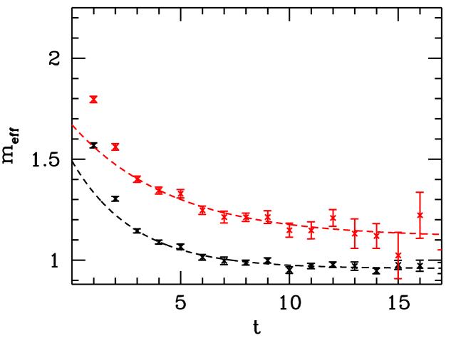
Figure 1: The effective masses for the first two states in the negative parity channel for $\kappa=0.1550$ and the fitted exponentials.

In both parity channels we extracted the two lowest masses (which we denote by $m_{0}$ and $m_{1}$). It is straightforward to define the ratio $\alpha_{i}=m_{i}/(m_{N}+m_{K})$ which compares the possible scattering and pentaquark states to the nucleon-kaon threshold. The experimental value of $\alpha$ for the $\Theta^{+}$ particle is $\alpha_{\Theta^{+}}=1.07$.

size	parity	$\kappa_{u,d}$	$am_{\pi}$	$am_{K}$	$am_{N}$	$\alpha_{0}$	$\alpha_{1}$
$24^{3}\times 60$	–	0.1550	0.296(1)	0.317(1)	0.642(6)	1.01(1)	1.16(5)
$24^{3}\times 60$	–	0.1555	0.259(1)	0.301(1)	0.613(5)	0.99(1)	1.16(5)
$24^{3}\times 60$	–	0.1558	0.234(1)	0.290(1)	0.592(6)	0.99(1)	1.14(8)
$24^{3}\times 60$	–	0.1563	0.185(1)	0.272(1)	0.545(7)	0.98(2)	1.28(13)
$20^{3}\times 60$	–	0.1550	0.295(1)	0.316(1)	0.647(7)	1.00(1)	1.24(8)
$24^{3}\times 60$	+	0.1550	0.295(1)	0.316(1)	0.636(6)	1.16(2)	1.45(16)
$24^{3}\times 60$	+	0.1555	0.258(2)	0.299(2)	0.615(14)	1.13(3)	1.39(15)
$24^{3}\times 60$	+	0.1558	0.233(2)	0.288(2)	0.595(12)	1.09(5)	1.39(17)
$24^{3}\times 60$	+	0.1563	0.184(3)	0.270(2)	0.552(10)	1.14(8)	1.31(32)
$20^{3}\times 60$	+	0.1550	0.295(1)	0.316(1)	0.647(6)	1.21(2)	1.48(12)

Table 2: The measured pion, kaon and nucleon masses and the ratio of the first two five-quark states in both parity channels to the $KN$ threshold.

The summary of our results including also the pion, kaon and nucleon masses is given in Table 2. The zero momentum scattering state is just at the threshold. The first scattering state with nonzero momentum is expected at

$$E_{1}=\sqrt{m_{K}^{2}+4\pi^{2}/(aN_{s})^{2}}+\sqrt{m_{N}^{2}+4\pi^{2}/(aN_{s})^{2}}.$$ (14)

Its ratio to the threshold is 1.151, 1.166, 1.177, 1.202 for $\kappa=0.1550,0.1555,0.1558$ and $0.1563$, respectively for our larger volume. For the smaller volume ($N_{s}=20$) at $\kappa=0.1550$ this ratio is $1.211$. We can see that in all cases the measured mass ratios are consistent with the scattering states. The expected and measured volume dependences of the first excited state for negative parity and the ground state for positive parity is shown in Fig. 2.

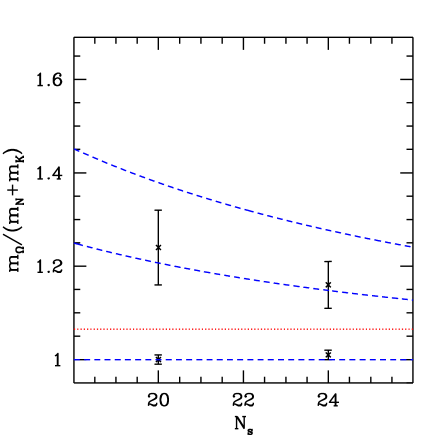
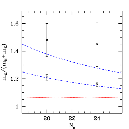
Figure 2: The volume dependence of the two lowest states in the two parity channels (left panel: negative parity; right panel: positive parity). The dashed lines indicate the expected scattering states with 0 momentum and the first two non-vanishing momenta. The dotted line shows the experimental value of the pentaquark state.

For the highest quark mass, where we had the largest statistics quark mass we also performed the whole analysis for the isovector channel. The extracted masses and their volume dependence turned out to be qualitatively similar to those in the isoscalar channel.

4 Conclusion

In this paper we studied spin 1/2 isoscalar and isovector, even and odd parity candidates for the $\Theta^{+}$ pentaquark using large scale lattice QCD simulations. The analysis needed approximately 0.5 Tflopyears of sustained 32 bit operations.

Before we summarize the results of the different channels one technical remark is in order. The $\Theta^{+}$ pentaquark is expected to be a few % above the NK threshold. Typical lattice sizes of a few fermis result in a discrete NK scattering spectrum, with order 10% energy difference between the lowest lying states. Thus, we are faced with two problems. First of all we have to find the possible pentaquark signal and the nearby scattering states. Secondly we have to tell the difference between them. Finding several states could be done by multi-parameter fitting or more effectively by spanning a multidimensional wave function basis and using a cross correlator technique. The most straightforward way to tell the difference between a narrow resonance and a scattering state is to use the fact that the former has an energy with quite weak volume dependence, whereas the latter has a definite volume dependence, defined by the momenta allowed in a finite system.

Clearly, any statement on the existence/non-existence or on the quantum numbers of the $\Theta^{+}$ pentaquark depends crucially on this sort of separation. None of the previous lattice investigations on the $\Theta^{+}$ pentaquark was able to carry out this analysis. The most important goal of the present paper was to do it.

The individual results in the odd and even parity channels can be summarized as follows (based on the statistically most significant, highest quark mass and assuming that $m_{\Theta}^{+}/(m_{N}+m_{K})$ scales with the quark mass).

1. Odd parity. The two lowest lying states are separated. The lower one is identified as the lowest scattering state with appropriate volume dependence (in this case the p=0 scattering means no volume dependence). This state is 6$\sigma$ below the $\Theta^{+}$ state. The volume dependence of the second lowest state is consistent with that of a scattering state with non-zero relative momentum. For our larger/smaller volumes this state is 1.8/1.3$\sigma$ above the $\Theta^{+}$ state. None of these two states could be interpreted as the $\Theta^{+}$ pentaquark.

2. Even parity. The two lowest lying states are identified. The volumes are chosen such that even the lowest lying scattering state is above the expected $\Theta^{+}$ pentaquark state. The volume dependence of the lowest state suggests that it is a scattering state. For both volumes this state is 6$\sigma$ above the $\Theta^{+}$ state. Since the energy of the second lowest state is even larger, none of them could be interpreted as the $\Theta^{+}$ pentaquark.

To summarize in both parity channels we identified all the nearby states both below and above the expected $\Theta^{+}$ state. Having done that no additional resonance state was found. This is an indication that in our wave function basis no $\Theta^{+}$ pentaquark exists (though it might appear in an even larger, more exotic basis, with smaller dynamical quark masses or approaching the continuum limit).

Appendix A Parity projection

In this appendix we summarize how the energy of the lowest state can be extracted separately in the two parity channels. Although we consider spin $1/2$ baryon correlators here, our discussion can be generalized to other states.

The basic objects one can compute on the lattice are Euclidean correlators of the form $\langle\,{\cal O}_{\alpha}(x)\bar{{\cal O}}_{\beta}(0)\,\rangle$ corresponding to the amplitude of the process of creating a state at time zero with the operator $\bar{{\cal O}}_{\beta}(0)$, evolving it to a later time $x_{0}$ and annihilating it with ${\cal O}_{\alpha}(x)$.

There are two complications when one wants to extract the lowest state in a given parity channel. Firstly, simple baryonic operators usually couple to both parities, therefore one has to project out parity by hand. Secondly, the box has a finite time extent $T$ with (anti)periodic boundary condition. Therefore, a single source at time zero is in fact mathematically equivalent to the sum of an infinite number of identical sources located at $t=0,\pm T,\pm 2T...$. Due to the exponential fall-off of correlations, only the two sources closest to the sink, i.e. at $t=0,T$ give appreciable contributions to the infinite sum. If we assume, as we shall always, that $0\leq x_{0}<T$ then

$$\sum_{n=-\infty}^{\infty}\langle\,{\cal O}_{\alpha}(\vec{x},x_{0})\bar{{\cal O}}_{\beta}(\vec{0},nT)\,\rangle\approx\langle\,{\cal O}_{\alpha}(\vec{x},x_{0})\bar{{\cal O}}_{\beta}(\vec{0},0)\,\rangle+\varepsilon_{\mbox{\scriptsize bc}}\langle\,{\cal O}_{\alpha}(\vec{x},x_{0})\bar{{\cal O}}_{\beta}(\vec{0},T)\,\rangle,$$ (15)

where $\varepsilon_{\mbox{\scriptsize bc}}$ is $+1$ for periodic and $-1$ for anti-periodic boundary condition in the time direction. The first term on the r.h.s. represents particles propagating from time $0$ to $x_{0}$ while the second term represents antiparticles propagating from time $x_{0}$ to $T$. Thus even after projecting to a given parity channel the correlator has contributions not only from particles of that parity, but also from the antiparticles of particles of the opposite parity. Therefore, an additional “projection” is needed to get rid of the latter.

Before starting to describe in detail how the two projections can be carried out let us discuss the form of the first term on the r.h.s. of eq. (15). We shall assume that ${\cal O}_{\alpha}$ is a spin $1/2$ baryon operator and $\alpha$ is its Dirac index. Due to the transformation properties of ${\cal O}_{\alpha}$, the most general form the correlator can have is

$$\langle\,{\cal O}_{\alpha}(x)\bar{{\cal O}}_{\beta}(0)\,\rangle=\left[\;f(x^{2})\,x_{\mu}\gamma^{\mu}+g(x^{2})\,{\bf 1}\;\right]_{\alpha\beta},$$ (16)

where $f$ and $g$ are scalar functions of the length of the four-vector $x$ and ${\bf 1}$ is the $4\times 4$ unit matrix. After projection to the zero momentum sector this becomes

$$C_{\alpha\beta}(x_{0})=\int\!\mbox{d}^{3}\!x\;\langle\,{\cal O}_{\alpha}(x)\bar{{\cal O}}_{\beta}(0)\,\rangle=\left[\,A(x_{0})\gamma_{0}+B(x_{0}){\bf 1}\,\right]_{\alpha\beta},$$ (17)

where

$$A(x_{0})=\int\!\mbox{d}^{3}\!x\;f(x^{2})x_{0},\hskip 28.45274ptB(x_{0})=\int\!\mbox{d}^{3}\!x\;g(x^{2}).$$ (18)

The important point here is that upon integration over 3-space the terms in the correlator proportional to the spacelike $\gamma$ matrices vanished due to their antisymmetry. We also note that from eq. (18) $A(x_{0})$ and $B(x_{0})$ are easily seen to be anti-symmetric and symmetric respectively.

Parity projection. Parity projection of an arbitrary operator ${\cal O}$ can be performed by

$${\cal P}_{\pm}{\cal O}=\frac{1}{2}\left({\cal O}\pm P{\cal O}P^{-1}\right),$$ (19)

where $P$ is the parity transformation and ${\cal P}_{\pm}{\cal O}$ couples to parity eigenstates of $\pm$ parity. In particular, on spin $1/2$ fermionic operators parity acts as

$$P{\cal O}_{\alpha}(x_{0},{\bf x})P^{-1}=\eta\,(\gamma_{0})_{\alpha\nu}\,{\cal O}_{\nu}(x_{0},-{\bf x}),$$ (20)

where $\eta=\pm 1$ is the internal parity of ${\cal O}$ depending on the parity convention we choose for the elementary fields and on how ${\cal O}$ is constructed from those. The analogous formula can be easily obtained for $\bar{{\cal O}}_{\alpha}$.

When constructing correlators it is enough to project to a given parity either at the sink or at the source. This by itself ensures that only states of the given parity are propagating in the correlator. Inserting the projection into the correlator of eq. (17) at the sink one obtains e.g. for the positive parity correlator

$$\frac{1}{2}\left({\bf 1}+\eta\gamma_{0}\right)\left[\,A(x_{0})\gamma_{0}+B(x_{0}){\bf 1}\,\right]=\frac{\eta}{2}\left[A(x_{0})+\eta B(x_{0})\right]{\bf 1}\;+\;\frac{1}{2}\left[A(x_{0})+\eta B(x_{0})\right]\gamma_{0}.$$ (21)

The negative parity channel can be constructed analogously by replacing $\eta$ with $-\eta$ everywhere.

Notice that all the matrix elements of the parity projected correlator have the same functional dependence, $1/2(A\pm\eta B)$, on $x_{0}$. The exponential fit to this function will yield the lowest state in the given parity channel. In practice the simplest way to obtain the parity projected correlator is to compute two suitable elements of the $4\times 4$ correlation matrix $C_{\alpha\beta}(x_{0})$ that yield $A(x_{0})$ and $B(x_{0})$ respectively. So far we pretended that the box is infinite in the time direction and neglected the second term on the r.h.s. of eq. (15).

“Particle” projection: Now the full correlator, including the term that “comes back” through the time boundary, the only object that we can actually compute in a finite box, has the form

$$C(x_{0})+\varepsilon_{\mbox{\scriptsize bc}}C(x_{0}-T)=\left[A(x_{0})-\varepsilon_{\mbox{\scriptsize bc}}A(T-x_{0})\right]\gamma_{0}\;+\;\left[B(x_{0})+\varepsilon_{\mbox{\scriptsize bc}}B(T-x_{0})\right]{\bf 1},$$ (22)

where we arranged the arguments of $A$ and $B$ to be non-negative using their (anti)-symmetry.

Were we to use our prescription above for parity projection, i.e. the “$\gamma_{0}$ component” of the correlator $\pm\eta\times$ its “${\bf 1}$ component”, we would end up with the parity projected correlator

$$\frac{1}{2}\left[A(x_{0})+\eta B(x_{0})\right]\;+\;\frac{\varepsilon_{\mbox{\scriptsize bc}}}{2}\left[-A(T-x_{0})+B(T-x_{0})\right],$$ (23)

which, due to an extra minus sign, does not have the simple functional form $f(x_{0})+f(T-x_{0})$ that could be fitted with a cosh. This extra sign, however, can be easily canceled if we compute the $A$ and the $B$ components (the one proportional to $\gamma_{0}$ and ${\bf 1}$, respectively in eq. (17)) with opposite boundary conditions. In that case the parity projected correlator has the form

$$\frac{1}{2}\left[A(x_{0})+\eta B(x_{0})\right]\;+\;\frac{1}{2}\left[A(T-x_{0})+\eta B(T-x_{0})\right].$$ (24)

If $1/2[A(x_{0})+\eta B(x_{0})]$ is a sum of exponentials corresponding to the energies of the states in the given channel, (24) is a sum of cosh’s with the same exponents. This is the functional form we have to use for fitting when extracting masses.

Appendix B Projection to a spin eigenstate

In this appendix we outline how a specific spin eigenstate can be projected out from a given lattice hadron operator. After summarizing the relevant group theoretical principles we discuss how our spin 1/2 pentaquark operators were constructed.

When discussing spin on a hypercubic lattice the first problem is that due to the absence of full $SO(3)$ rotational symmetry it is not straightforward to assign spin to a lattice energy eigenstate. States on the lattice can be classified into irreducible representations of the cubic group $O$ or its double cover ${}^{2}O$, not $SO(3)$ and $SU(2)$ as in the continuum.

With the exception of the lowest four representations, when restricted to ${}^{2}O$, irreducible representations of $SU(2)$ do not remain irreducible. The spin 0, 1/2, 1 and 3/2 $SU(2)$ representations are the exceptions, these restricted to ${}^{2}O$ are equivalent to the irreducible representations $A_{1},G_{1},T_{1}$ and $H$, respectively. Also any state belonging to an irreducible representation of ${}^{2}O$ has components belonging to several different spin representations of $SU(2)$. For instance a state in $G_{1}$ has components in spin $1/2,7/2,9/2...$ $SU(2)$ representations and $H$ has components of spin $3/2,5/2,7/2...$.

This means e.g. that if on the lattice we find the lowest energy state in the $G_{1}$ representation of ${}^{2}O$, we can identify that with a spin 1/2 state in the continuum, provided all the higher spin states contributing to $G_{1}$, i.e. $s=7/2,9/2...$ can be assumed to have much higher energy. In this sense, for practical purposes, the lowest few representations of $SU(2)$ and ${}^{2}O$ can be identified as follows:

$$0\leftrightarrow A_{1},\hskip 8.53581pt1/2\leftrightarrow G_{1},\hskip 8.53581pt1\leftrightarrow T_{1},\hskip 8.53581pt3/2\leftrightarrow H.$$ (25)

The task we have at hand is thus to construct states belonging to specific representations of the cubic group ${}^{2}O$. This can be most easily done using the technique of projection operators that we summarize here for completeness. The simple form of the method of projectors we present here can be used only when each irreducible representation occurs in the decomposition at most once. Therefore it is essential to know ahead of time the irreducible representations occurring in a tensor product and their multiplicities. This can be most easily found using group characters. See e.g. [46] for explicit formulae and character tables of $O$ and ${}^{2}O$.

Let $G$ be a finite group, $D^{(r)}_{ij}(g)$ be the matrix elements of its irreducible representation $r$ of dimension $d_{r}$. Let the transformations $T(g)$ form an arbitrary (not necessarily irreducible) unitary representation of $G$. We would like to project a specific irreducible representation $r$ out of the carrier space of the $T(g)$’s. Let us define the transformations

$$P^{(r)}_{ij}=\frac{d_{s}}{|G|}\sum_{g\in G}D^{(r)\star}_{ij}(g)\;T(g),$$ (26)

where $|G|$ is the number of elements $G$ has and ^⋆ denotes complex conjugation.

It is straightforward to show that if $|\psi\rangle$ is any vector belonging to the carrier space of $T(g)$’s then for a fixed $j$ the $d_{r}$ vectors

$$|\phi_{i}\rangle=P^{(r)}_{ij}|\psi\rangle,\hskip 8.53581pti=1,...d_{r}$$ (27)

either transform as basis vectors of the irreducible representation $r$ or they are all zero. For the proof see any standard text on group representations, e.g. Ref. [45]. Equations (26) and (27) can be exploited to project out different representations of ${}^{2}O$ from a given state on the lattice and its rotated copies.

In particular, we would like to construct pentaquark states belonging to $G_{1}$ that corresponds to spin 1/2. Although more complicated cases can also be considered, here we restrict ourselves to the one where the spin indices of all the quarks but one have been contracted to be scalars and the total spin of the pentaquark arises by combining the spin 1/2 ($G_{1}$) of the remaining quark with the orbital angular momentum of all the constituents. Therefore we have to project $G_{1}$ out of $G_{1}\otimes s$, where $s$ is a representation of the cubic group $O$ (not ${}^{2}O$!), corresponding to the orbital part.

In practice $s$ depends on the spatial arrangement of quark sources and this can be exploited to make things as simple as possible. Eq. (26) implies that, in general, projection to a specific spin involves as many terms as the number of elements of the group ${}^{2}O$, i.e. 48. The situation, however, is much better if the projection formula (27) is applied to a state, with an orbital part having some degree of symmetry under cubic rotations. The simplest case is when the five quark sources all have complete rotational symmetry, i.e. the orbital part is trivially $s=A_{1}$. Then all the rotated copies of the quark sources are identical, the sum in eq. (26) can be explicitly computed and the projection reduces to projection to spin up or spin down. The decomposition here is $A_{1}\otimes G_{1}=G_{1}$. All the operators used in lattice pentaquark spectroscopy so far fall into this category.

To explore the possibility of non-zero orbital angular momentum we have to consider less symmetric quark sources. Another possibility is to put the antiquark at the origin with a rotationally symmetric wave function, displace the two pairs of $(ud)$ quarks along a coordinate axis (say $z$) keeping the arrangement cylindrically symmetric with respect to the $z$ axis. Inspired by the Jaffe-Wilczek diquark-diquark-antiquark picture [26], in anticipation of orbital angular momentum 1, we construct this state to be antisymmetric with respect to the interchange of the two displaced quark pairs. Let us call such a state $|\pm z\rangle$. It is easy to see that the rotated copies of this state span a three dimensional space carrying the representation $T_{1}$ of $O$. A possible set of basis states is given by $(ud)$ pairs displaced along the three coordinate axes; $|\pm x\rangle,|\pm y\rangle,|\pm z\rangle$. This arrangement corresponds to projecting out the spin $1/2$ $(G_{1})$ component from the decomposition

$$T_{1}\otimes G_{1}=G_{1}\oplus H.$$ (28)

Let us choose $|\psi\rangle=|\!\uparrow\rangle\otimes|\pm z\rangle$ and compute $P_{11}^{(G_{1})}|\psi\rangle$. The transformations $T(g)$ appearing in eq. (26) are direct products of $G_{1}$ transformations acting on the quark spin and transformations acting on the orbital part. Each term in the sum and as a consequence the whole sum itself can be decomposed into three terms proportional to $|\pm x\rangle,|\pm y\rangle$ and $|\pm z\rangle$. The $G_{1}$ matrices can be easily obtained by restricting the defining representation of $SU(2)$ to ${}^{2}O$ and with the factors $D^{(G_{1})\star}_{ij}(g)$ they can be summed independently for the three terms resulting in

$$P_{11}^{(G_{1})}\;\left[|\!\uparrow\rangle\otimes|\pm z\rangle\right] = {\left(\begin{array}[]{cc}0&0\\ 1&0\end{array}\right)}|\!\uparrow\rangle\otimes|\pm x\rangle+{\left(\begin{array}[]{cc}0&0\\ i&0\end{array}\right)}|\!\uparrow\rangle\otimes|\pm y\rangle+{\left(\begin{array}[]{cc}1&0\\ 0&0\end{array}\right)}|\!\uparrow\rangle\otimes|\pm z\rangle$$ (35)

$$= |\!\downarrow\rangle\otimes|\pm x\rangle+i|\!\downarrow\rangle\otimes|\pm y\rangle+|\!\uparrow\rangle\otimes|\pm z\rangle.$$ (36)

In a similar fashion we obtain the other (spin down) basis element of the $G_{1}$ projection;

$$P_{21}^{(G_{1})}\;\left[|\!\uparrow\rangle\otimes|\pm z\rangle\right]\;=\;|\!\uparrow\rangle\otimes|\pm x\rangle\;-\;i|\!\uparrow\rangle\otimes|\pm y\rangle\;-\;|\!\downarrow\rangle\otimes|\pm z\rangle.$$ (37)

Note that, up to some numerical factors coming from the normalization of spherical harmonics, these expressions are identical to the spin $1/2$ part of the $SU(2)$ Clebsch-Gordan decomposition $1\otimes 1/2=1/2\oplus 3/2$. We could also construct spin 1/2 from similar, but symmetric orbital states for the quarks displaced to $x,y,z=-d$. This would correspond to $A_{1}\otimes G_{1}=G_{1}$ or $0\otimes 1/2=1/2$ for $SU(2)$.

Building these states requires seven quark sources; an antiquark at the origin and six quark sources, two along each coordinate axis (we use the same mass and source for the $u$ and $d$ quarks). Eq. (28) shows that keeping the same spatial arrangement the representation $H$ corresponding to spin $3/2$ could also be projected out. However, we have not explored this possibility here. For that we would have had to replace the matrix elements $D^{(G_{1})\star}_{ij}(g)$ in eq. (26) with those of $H$.

Besides the diquark-diquark-antiquark wave function we also wanted to study triquark quark-antiquark states. The simplest non-trivial way to do that is to displace the quark-antiquark pair along a coordinate axis, say $+z$. Let us call the orbital part of this state $|+z\rangle$. Its rotated copies span the six dimensional space with a possible basis formed by $|+x\rangle,|-x\rangle,|+y\rangle,|-y\rangle,|+z\rangle,|-z\rangle$. This space, however, can be split into an antisymmetric part spanned by combinations of the form $|+x\rangle-|-x\rangle,...$ and a symmetric one spanned by $|+x\rangle+|-x\rangle,$ etc. The representation of $O$ on the antisymmetric part is $T_{1}$ in exactly the same way as in the diquark-diquark case, resulting again in the spin projected state

$$P_{11}^{(G_{1})}\;\left[|\!\uparrow\rangle\otimes(|+z\rangle-|-z\rangle)\right]=\hskip 142.26378pt$$

$$|\!\downarrow\rangle\otimes(|+x\rangle-|-x\rangle)\;+\;i|\!\downarrow\rangle\otimes(|+y\rangle-|-y\rangle)\;+\;|\!\uparrow\rangle\otimes(|+z\rangle-|-z\rangle).$$ (38)

The three dimensional symmetric part of the orbital space is reducible to $A_{1}\oplus E$. Thus we can also produce spin 1/2 trivially from the symmetric part by $A_{1}\otimes G_{1}=G_{1}$,

$$P_{11}^{(G_{1})}\;\left[|\!\uparrow\rangle\otimes(|+z\rangle+|-z\rangle)\right]=\hskip 142.26378pt$$

$$|\!\uparrow\rangle\otimes\left[|+x\rangle+|-x\rangle+|+y\rangle+|-y\rangle+|+z\rangle+|-z\rangle\right].$$ (39)

- [1] T. Nakano et al., Phys. Rev. Lett. 91, 012002 (2003). [arXiv:hep-ex/0301020].
- [2] S. Stepanyan et al. [CLAS Collaboration], Phys. Rev. Lett. 91, 252001 (2003). [arXiv:hep-ex/0307018].
- [3] J. Barth et al. [SAPHIR Collaboration], Phys. Lett. B572, 127 (2003). [arXiv:hep-ex/0307083].
- [4] V. V. Barmin et al. [DIANA Collaboration], Phys. Atom. Nucl. 66, 1715 (2003); Yad. Fiz. 66, 1763 (2003). [arXiv:hep-ex/0304040].
- [5] A.E. Asratyan, A.G. Dolgolenko, and M.A. Kubantsev, Phys. Atom. Nucl. 67, 682 (2004); Yad. Fiz. 67, 704 (2004).
- [6] V. Kubarovsky et al. CLAS Collaboration, Phys. Rev. Lett. 92, 032001 (2004); erratum ibid. 92, 049902 (2004).
- [7] A. Airapetian et al. HERMES Collaboration, Phys. Lett. B585, 213 (2004).
- [8] S. Chekanov et al. ZEUS Collaboration, Phys. Lett. B591, 7 (2004).
- [9] A. Aleev et al. SVD Collaboration, hep-ex/0401024.
- [10] M. Abdel-Bary et al. COSY-TOF Collaboration, Phys. Lett. B595, 127 (2004).
- [11] P.Zh. Aslanyan, V.N. Emelyanenko and G.G. Rikhkvizkaya, hep-ex/0403044.
- [12] Yu.A. Troyan et al., hep-ex/0404003.
- [13] J. Z. Bai et al. [BES Collaboration], Phys. Rev. D 70 (2004) 012004 [arXiv:hep-ex/0402012].
- [14] K. T. Knopfle, M. Zavertyaev and T. Zivko [HERA-B Collaboration], J. Phys. G 30 (2004) S1363 [arXiv:hep-ex/0403020].
- [15] C. Pinkenburg [PHENIX Collaboration], J. Phys. G 30 (2004) S1201 [arXiv:nucl-ex/0404001].
- [16] M. J. Longo et al. [HyperCP Collaboration], Phys. Rev. D 70 (2004) 111101 [arXiv:hep-ex/0410027].
- [17] D. O. Litvintsev [CDF Collaboration], [arXiv:hep-ex/0410024].
- [18] T. Berger-Hryn’ova [BaBar Collaboration], [arXiv:hep-ex/0411017].
- [19] K. Abe et al. [Belle Collaboration], [arXiv:hep-ex/0411005].
- [20] S. R. Armstrong, [arXiv:hep-ex/0410080].
- [21] P. Rossi [CLAS Collaboration], [arXiv:hep-ex/0409057].
- [22] C. Alt et al. [NA49 Collaboration], Phys. Rev. Lett. 92 (2004) 042003 [arXiv:hep-ex/0310014];
- [23] A. Aktas et al. [H1 Collaboration], Phys. Lett. B 588 (2004) 17 [arXiv:hep-ex/0403017].
- [24] D. Diakonov, V. Petrov and M. V. Polyakov, Z. Phys. A 359, 305 (1997) [arXiv:hep-ph/9703373]; M. V. Polyakov and A. Rathke, Eur. Phys. J. A 18, 691 (2003) [arXiv:hep-ph/0303138]. H. Walliser and V. B. Kopeliovich, J. Exp. Theor. Phys. 97, 433 (2003) [Zh. Eksp. Teor. Fiz. 124, 483 (2003)] [arXiv:hep-ph/0304058]. D. Borisyuk, M. Faber and A. Kobushkin, [arXiv:hep-ph/0307370]. H. C. Kim and M. Praszalowicz, Phys. Lett. B 585, 99 (2004) [arXiv:hep-ph/0308242].
- [25] M. Praszałowicz, talk at Workshop on Skyrmions and Anomalies, M. Jeżabek and M. Praszałowicz eds., World Scientific 1987, page 112 and Phys. Lett. B575 (2003) 234 [hep-ph/0308114].
- [26] R. L. Jaffe and F. Wilczek, Phys. Rev. Lett. 91, 232003 (2003) [arXiv:hep-ph/0307341], hep-ph/0312369.
- [27] K. Cheung, Phys. Rev. D 69, 094029 (2004) [arXiv:hep-ph/0308176]. R. D. Matheus, F. S. Navarra, M. Nielsen, R. Rodrigues da Silva and S. H. Lee, Phys. Lett. B 578, 323 (2004) [arXiv:hep-ph/0309001].
- [28] F. Stancu and D. O. Riska, Phys. Lett. B 575, 242 (2003) [arXiv:hep-ph/0307010].
- [29] M. Karliner and H. J. Lipkin, Phys. Lett. B 575 (2003) 249 [arXiv:hep-ph/0402260]. L. Y. Glozman, Phys. Lett. B 575, 18 (2003) [arXiv:hep-ph/0308232]; S. Capstick, P. R. Page and W. Roberts, Phys. Lett. B 570, (2003) 185; B. G. Wybourne, hep-ph/0307170; A. Hoska, Phys. Lett. B 571, (2003) 55; V. E. Lyubovitskij, P. Wang, Th. Gutsche, A. Faessler, Phys. Rev. C66 (2002) 055204; B. K. Jennings and K. Maltman, Phys. Rev. D 69 (2004) 094020 [arXiv:hep-ph/0308286]. C. E. Carlson, C. D. Carone, H. J. Kwee and V. Nazaryan, Phys. Lett. B 573, 101 (2003) [arXiv:hep-ph/0307396]; C. E. Carlson, C. D. Carone, H. J. Kwee and V. Nazaryan, Phys. Lett. B579 (2004) 52; C. E. Carlson, C. D. Carone, H. J. Kwee and V. Nazaryan, Phys. Rev. D 70 (2004) 037501 [arXiv:hep-ph/0312325]; F. Huang, Z. Y. Zhang, Y. W. Yu and B. S. Zou, Phys. Lett. B 586 (2004) 69 [arXiv:hep-ph/0310040]; I. M. Narodetskii, Yu. A. Simonov, M. A. Trusov and A. I. Veselov, Phys. Lett. B578, (2004) 318; S. M. Gerasyuta and V. I. Kochkin, hep-ph/0310225; hep-ph/0310227; R. Bijker, M. M. Giannini and E. Santopinto, Eur. Phys. J. A 22 (2004) 319 [arXiv:hep-ph/0310281]; R. Bijker, M. M. Giannini and E. Santopinto, Rev. Mex. Fis. 50S2 (2004) 88 [arXiv:hep-ph/0312380].
- [30] N. Itzhaki, I. R. Klebanov, P. Ouyang and L. Rastelli, Nucl. Phys. B 684 (2004) 264 [arXiv:hep-ph/0309305]; D. E. Kahana and S. H. Kahana, Phys. Rev. D 69 (2004) 117502 [arXiv:hep-ph/0310026]; F. J. Llanes-Estrada, E. Oset and V. Mateu, Phys. Rev. C 69 (2004) 055203 [arXiv:nucl-th/0311020].
- [31] S. L. Zhu, Phys. Rev. Lett. 91, 232002 (2003) [arXiv:hep-ph/0307345]. J. Sugiyama, T. Doi and M. Oka, Phys. Lett. B 581, 167 (2004) [arXiv:hep-ph/0309271]. Y. Kondo, O. Morimatsu and T. Nishikawa, arXiv:hep-ph/0404285; S. H. Lee, H. Kim and Y. Kwon, [arXiv:hep-ph/0411104]; P. Z. Huang, W. Z. Deng, X. L. Chen and S. L. Zhu, Phys. Rev. D 69 (2004) 074004 [arXiv:hep-ph/0311108].
- [32] F. Csikor, Z. Fodor, S. D. Katz and T. G. Kovacs, JHEP 0311, 070 (2003). [arXiv:hep-lat/0309090].
- [33] S. Sasaki, Phys. Rev. Lett. 93, 152001 (2004). [arXiv:hep-lat/0310014].
- [34] T. W. Chiu and T. H. Hsieh, hep-ph/0403020; hep-ph/0404007.
- [35] T. T. Takahashi, T. Umeda, T. Onogi and T. Kunihiro, hep-lat/0410025.
- [36] N. Mathur et al., Phys. Rev. D70, 074508 (2004). [arXiv:hep-ph/0406196].
- [37] N. Ishii, T. Doi, H. Iida, M. Oka, F. Okiharu and H. Suganuma, Phys. Rev. D71, 0340001 (2005).
- [38] C. Alexandrou, G. Koutsou and A. Tsapalis, hep-lat/0409065.
- [39] F. Csikor, Z. Fodor, S. D. Katz and T.G. Kovacs, hep-lat/0407033; S. Sasaki, arXiv:hep-lat/0410016.
- [40] C. Gattringer et al. [BGR Collaboration], Nucl. Phys. B 677, 3 (2004) [arXiv:hep-lat/0307013].
- [41] S. Aoki et al. [CP-PACS Collaboration], Phys. Rev. D 67, 034503 (2003) [arXiv:hep-lat/0206009].
- [42] C. R. Allton, V. Gimenez, L. Giusti and F. Rapuano, Nucl. Phys. B 489, 427 (1997) [arXiv:hep-lat/9611021].
- [43] H. P. Shanahan et al. [UKQCD Collaboration], Phys. Rev. D 55, 1548 (1997) [arXiv:hep-lat/9608063].
- [44] C. J. Morningstar and M. J. Peardon, Phys. Rev. D 56 (1997) 4043 [arXiv:hep-lat/9704011], Phys. Rev. D 60 (1999) 034509 [arXiv:hep-lat/9901004].
- [45] A.O. Barut and R. Raczka, Theory of group representations and applications, PWN Scientific Publishers, Warszawa 1980, p. 178.
- [46] R. C. Johnson, Phys. Lett. B 114 (1982) 147.