Warped Domain Wall Fermions

Abstract:

We consider Kaplan’s domain wall fermions in the presence of an Anti-de Sitter (AdS) background in the extra dimension. Just as in the flat space case, in a completely vector-like gauge theory defined after discretizing this extra dimension, the spectrum contains a very light charged fermion whose chiral components are localized at the ends of the extra dimensional interval. The component on the IR boundary of the AdS space can be given a large mass by coupling it to a neutral fermion via the Higgs mechanism. In this theory, gauge invariance can be restored either by taking the limit of infinite proper length of the extra dimension or by reducing the AdS curvature radius towards zero. In the latter case, the Kaluza-Klein modes stay heavy and the resulting classical theory approaches a chiral gauge theory, as we verify numerically. Potential difficulties for this approach could arise from the coupling of the longitudinal mode of the light gauge boson, which has to be treated non-perturbatively.

1 Introduction

Though exact regularizations of chiral gauge theories in the Higgs phase have long been considered [1], the non-perturbative definition of unbroken chiral gauge theories has remained a vexing problem. The most natural attempts to discretize the theory on a space-time lattice ran up against the famous Nielsen-Ninomiya no-go theorem [2] which states that no discretization of the Euclidean 4D Dirac operator can have the correct free fermion spectrum and dispersion relation in the continuum limit if it is translationally invariant, local, and chirally invariant. Ginsparg and Wilson [3] realized that a possible way out was to violate the chiral symmetry mildly, i.e., the anti-commutator of the fermion propagator with $\gamma_{5}$ could be made zero at all non-zero distances, and explicit realizations of this form have recently been found [4]. Lüscher [5] showed that the Ginsparg-Wilson relation implied an exact lattice symmetry which reduced to the chiral symmetry in the naïve continuum limit, but this symmetry depended on the interactions of the fermion. Such a structure allows a consistent chiral projection of the theory, but the interaction dependence has hindered an explicit discretization of the projected fermions involved in unbroken chiral gauge interactions. The current attempts at defining such a theory, therefore, hinge on directly defining the fermion measure [6], or on fixing the gauge symmetry on the lattice only to restore it in the continuum [7, 8]. Obtaining this regularization directly as a limit of more standard gauge invariant discretizations could possibly provide better understanding of its nonperturbative aspects, and is the goal of this paper.

Kaplan [9] has shown that fermions in a 5D gauge theory can have 4D almost-zero modes whose opposite chirality components are localized at different positions in the 5D bulk. Since the 4D Dirac operator defined on the Kaluza-Klein modes of this theory does not satisfy the assumptions of the Nielsen-Ninomiya no-go theorem, it would seem that if one could further localize the gauge field around one of these zero modes, say the left-handed one, then one would have a chiral gauge theory on the lattice. Having a gauge interaction turned on where the left-handed fermion is localized and turning this interaction off somewhere in between this position and that of the right-handed fermion, however, has been shown to result in two new zero modes [10] with opposite chiralities, exactly one of which couples to the 4D gauge zero mode rendering the theory vector-like. It has been noted that one could try to decouple the extra fermions by adding Yukawa couplings and an appropriate Higgs vacuum expectation value (VEV), but that taking the VEV large enough to decouple the fermions would also make the gauge boson heavy [10] and thus result in a spontaneously broken gauge theory rather than the long sought after unbroken chiral gauge theory.

Recent developments [11, 12, 13, 14] in the phenomenology of electroweak symmetry breaking seem to offer a way out. In theories with an extra dimension, there are gauge boson modes that vanish at a boundary, and these are not affected by a VEV localized there. As a result even in the infinite VEV limit there are modes of the gauge boson which stay finite in mass, decouple from the Higgs, and result in unitary scattering without any contribution from the Higgs [12, 15]. Finally, when the extra dimension is a warped space, such as 5D Anti-de Sitter (AdS₅), the limit of zero curvature radius makes the lightest of these modes massless, leaving the rest of the Kaluza-Klein spectrum heavy. Thus, it seems we can have our cake: a gauge-breaking fermion mass, and eat it too: an arbitrarily light gauge boson with no light Kaluza-Klein modes. In this paper we will show explicity how to latticize the extra dimension and discuss how to take a limit of this vector-like gauge theory that becomes a chiral gauge theory at the classical level.

We start with a brief review of Kaplan’s original domain wall fermion idea in Section 2, and review, in the next section, the arguments that suggest that it is impossible to decouple one of the localized light modes without either having new light fermions pop up, or giving a large mass to the gauge boson. Next, we review fermions in warped extra dimensions, and present the continuum version of chiral warped domain wall fermions. In Section 5 we discuss the discretization of the extra dimension and the required scalings, while in Section 6 we demonstrate that the classical discretized theory with fermions is indeed chiral. The main worry about this proposal is the effect of the longitudinal component of the gauge field, which becomes strongly coupled near the IR brane. This is discussed in Section 7. Section 8 contains comments about a first attempt to latticize the remaining four dimensions without violating the underlying AdS symmetries. Finally issues regarding anomalies and instantons are discussed in Section 9.

2 Review of the Kaplan domain wall fermion proposal

Let us start our discussion with an overview of fermions in an extra dimension, and with it the domain wall approach proposed by Kaplan. The Lorentz group in 5D is bigger than the 4D Lorentz group, and the 5D Clifford algebra, by definition, also includes $\gamma_{5}$. An irreducible fermion representation of the 5D Lorentz group has to contain both chiralities, and a 5D theory is, therefore, non-chiral, as long as 5D Lorentz invariance is not broken. A generic 5D fermion action in flat space can be written as

$$S=\int d^{5}x\left(-i\bar{\chi}\bar{\sigma}^{\mu}\partial_{\mu}\chi-i\psi\sigma^{\mu}\partial_{\mu}\bar{\psi}+\frac{1}{2}(\psi\overleftrightarrow{\partial_{5}}\chi-\bar{\chi}\overleftrightarrow{\partial_{5}}\bar{\psi})+m\left(\psi\chi+\bar{\chi}\bar{\psi}\right)\right)\,,$$ (2.1)

where $\psi$ and $\chi$ are the two-component Weyl spinors corresponding to the chiral components making up a Dirac spinor. We will call $\psi$ the left, and $\chi$ the right, chiral component in this paper. Since the theory is vectorlike, a 5D “bulk mass” is allowed, and is denoted by $m$ here. The above action simply follows from writing out the 5D action

$$\int d^{5}x\bar{\Psi}(i\Gamma_{M}\partial^{M}+m)\Psi\,,$$ (2.2)

($M=0,1,2,3,5$) in terms of 4D components

$$\Psi=\left(\begin{array}[]{c}\chi\\ \bar{\psi}\end{array}\right)\,,$$ (2.3)

and using $\Gamma_{\mu}=\gamma_{\mu}$, $\Gamma_{5}=i\gamma_{5}$ ($\mu=0,1,2,3$) in the usual Dirac basis for the Clifford algebra.

One can distinguish between the left and right chiralities of the fermions by breaking 5D Lorentz invariance in some way. The mechanism proposed by Kaplan was to consider a kink generated by a scalar $\phi$ in the extra dimension. In this kink background there will be a single zero mode with definite chirality localized around the center of the kink. To see this, assume that the Lagrangian is of the form

$$\int d^{5}x\bar{\Psi}(i\gamma_{M}\partial^{M}+\phi(y))\Psi\,,$$ (2.4)

where the background $\phi(y)$ is such that $\phi(y)\to-v_{0}$ for $y\to-\infty$ and $\phi(y)\to v_{0}$ for $y\to\infty$, and $\phi(y_{0})=0$. The equation of motion in terms of the two component spinors will then be:

$$-i\bar{\sigma}^{\mu}\partial_{\mu}\chi-\partial_{5}\bar{\psi}+\phi(y)\bar{\psi}=0\,,$$

$$-i\sigma^{\mu}\partial_{\mu}\bar{\psi}+\partial_{5}\chi+\phi(y)\chi=0\,.$$ (2.5)

In order to find the 4D modes that solve these equations we write down the KK decomposition for the 5D spinors:

$$\chi=\sum_{n}g_{n}(y)\,\chi_{n}(x)\,,$$ (2.6)

$$\bar{\psi}=\sum_{n}f_{n}(y)\,\bar{\psi}_{n}(x)\,,$$ (2.7)

where $\chi_{n}$ and $\psi_{n}$ are two-component 4D spinors which form a Dirac spinor of mass $m_{n}$ and satisfy the 4D Dirac equation:

$$-i\bar{\sigma}^{\mu}\partial_{\mu}\chi_{n}+m_{n}\,\bar{\psi}_{n}=0\,,$$ (2.8)

$$-i\sigma^{\mu}\partial_{\mu}\bar{\psi}_{n}+m_{n}\,\chi_{n}=0\,.$$ (2.9)

Plugging this expansion into the bulk equations we get the following set of coupled first order differential equations for the wave functions $f_{n}$ and $g_{n}$:

$$g_{n}^{\prime}+\phi(y)\,g_{n}-m_{n}\,f_{n}=0\,,$$ (2.10)

$$f_{n}^{\prime}-\phi(y)\,f_{n}+m_{n}\,g_{n}=0\,.$$ (2.11)

For zero modes $m_{n}=0$, and we get two decoupled first order equations which can be immediately solved [9, 17]:

$$g_{0}^{\prime}+\phi(y)\,g_{0}=0;\ \ g_{0}(y)\propto e^{-\int_{-\infty}^{y}\phi(y^{\prime})dy^{\prime}}$$ (2.12)

$$f_{0}^{\prime}-\phi(y)\,f_{0}=0;\ \ f_{0}(y)\propto e^{\int_{-\infty}^{y}\phi(y^{\prime})dy^{\prime}}\,.$$ (2.13)

If the extra dimension is infinite, then only one of the two zero mode wave function chiralities will be normalizable, and thus we have achieved our goal of generating a chiral theory starting from a totally non-chiral one. In the case of a kink with $\phi\to-v_{0}$ for $y\to-\infty$ we find that only the function $g_{0}$ is normalizable, so there is a zero mode in $\chi$, while for an anti-kink the situation would be reversed.

3 The Golterman-Shamir no-go arguments against a chiral domain wall fermion theory

In the previous section, we obtained a chiral theory from a completely vectorlike model. It, however, does not look like a 4D theory even at long distances, since there is a continuum of 4D fermion and gauge boson modes. In order to make the theory at low energies look like a 4D theory, we need to consider the theory on a finite interval or assume boundary conditions (BC’s) with similar effects. Since the chirality was achieved by pushing one of the modes to infinity, as soon as we depart from the strictly infinite extra dimension, the theory will become non-chiral again. One simple example to explain this is to consider the case when the extra dimension is made finite by imposing periodic BC’s in the extra dimensional coordinate $y$. In that case $\phi(y)$ is periodic too, so if there is a kink at $y_{0}$ there needs to be an anti-kink somewhere else. In this case the anti-kink will support a zero-mode of opposite chirality (in fact the modes at the kink and anti-kink will interact and there will not be any exact zero modes) and the theory will not be chiral.

Let us discuss this issue in more detail in terms of a theory discretized along the extra dimension but still left in the continuum limit along the four transverse dimensions. This is commonly referred to as a theory with a deconstructed extra dimension [18]. Let us have as our starting point a theory on a finite interval $0<y<L$, and with a bulk mass for the fermions $m$. For this case (2.12) can still be applied (with $\phi(y)=m$) to find the two possible zero mode solutions [21]:

$$g_{0}(y)=e^{-my}$$ (3.1)

$$f_{0}(y)=e^{my}\,.$$ (3.2)

These two possible zero modes of opposite chiralities are localized on the opposite ends of the extra dimension. Thus we can see that a simple bulk mass in a finite interval acts exactly like a domain wall and one does not need to complicate the discussion by involving a scalar field profile.

To make the Hamiltonian self-adjoint, one needs to enforce appropriate boundary conditions. In the continuum 5D theory one can consistently impose Dirichlet boundary condition of the form

$$\psi(0)=0\qquad\hbox{or}\qquad\psi(L)=0\,,$$ (3.3)

(or the same BC for $\chi$). In this case the zero mode for $\psi$ (respectively, $\chi$) would be eliminated, leaving us with a chiral theory on a finite interval. A similar condition on the deconstructed theory would seem to run afoul of the Nielsen-Ninomiya theorem [2], and would, thus, be a barrier to further latticizing the four dimensional slices on the boundaries. We therefore do not introduce such boundary conditions and work in the theory where both zero-modes are present.

An explicit construction for the fermions is given by the following deconstructed action [22]:

$$\sum_{i=1}^{N}[-i\bar{\chi}_{i}\bar{\sigma}^{\mu}\partial_{\mu}\chi_{i}-i\psi_{i}\sigma^{\mu}\partial_{\mu}\bar{\psi}_{i}]+\sum_{i=1}^{N-1}\frac{1}{a}[\psi_{i+1}(\chi_{i+1}-\chi_{i})+ma\,\psi_{i+1}\chi_{i+1}]\,.$$ (3.4)

Here $a$ is the lattice spacing, $i$ labels the sites in the fifth direction, and $Na=L$. The structure of this action is schematically depicted in Fig. 1. We have initially chosen not to add a link between the first $\psi$ and $\chi$ fields, since for this set of masses it is quite simple to understand the spectrum of zero modes. The construction can then be extended via adding the extra link. In this particular choice we have made it is quite clear that there have to be two exact zero modes in the spectrum. Since $\psi_{1}$ has no mass term at all, it is massless. Of the remaining fields there are $N-1$ left handed and $N$ right handed fields, so one combination of the right handed $\chi$ fields also needs to be massless. In fact it is easy to find the zero mode of the mass matrix

$$M=\frac{1}{a}\left(\begin{array}[]{ccccc}{}{}\hfil&{}\hfil&\\ -1&1+ma\\ &-1&1+ma\\ &&\ddots&\ddots\\ &&&-1&1+ma\end{array}\right)\,.$$ (3.5)

The zero mode is given by

$$\chi_{i}=(1+ma)^{-i}\,,$$ (3.6)

which is just the discretized version of one of the continuum zero mode wave functions $e^{-my}$.

Of course it is quite unnatural not to add the mass term on the first site. Using the above analysis of zero modes in the absence of $m\psi_{1}\chi_{1}$ one can however understand easily the effect of adding this operator to the Lagrangian in (3.4). In the model without this term the $\psi$ zero mode is always at the first site $\psi_{1}$, while the $\chi$ zero mode is exponentially increasing (for $m<0$) or exponentially decreasing (for $m>0$) away from $\chi_{1}$. Thus adding the $\psi_{1}\chi_{1}$ mass term will totally remove the zero modes if $m>0$, since in that case it is a mass term for two zero modes localized almost at the same location. However, for $m<0$ adding this term will only have a small effect on the $\chi$ zero mode, since that has a very small overlap with $\chi_{1}$, and so one still expects an extremely light Dirac particle in the spectrum, whose mass is exponentially suppressed compared to all the other modes. This very light Dirac mode (whose $\psi$ component is mostly $\psi_{1}$ and whose $\chi$ component is mostly $\chi_{N}$) will be the approximate Kaplan domain wall fermion.

Figure 1: The deconstruction of a fermions in a flat extra dimension. The empty circles denote left handed two component fermions, while the filled circles denote right handed ones. A link between two circles indicates that a mass term is present connecting the two fermions, either from the bulk mass term, or from the discretization of the 5D derivative piece.

Let us now discuss what happens in the presence of a gauge field. We consider for now a gauge field which does not fluctuate in the fifth direction so that there is one $SU(n)$ symmetry under which all the fermions transform. We do not have a chiral gauge theory since there are two very light fermion modes of opposite chiralities localized at the two ends of the interval, and both of them couple equally strongly to the gauge field.

To remedy this situation, two proposals were studied by Golterman et al. [10]:

$\bullet$ The gauge field does not propagate everywhere, but only in a region (called the wave guide) around the first site, this way the second zero mode does not have a gauge coupling.

$\bullet$ The gauge field is Higgsed at the last site where the opposite chirality fermion zero mode lives and the second zero mode gets a mass with some gauge singlet fermion on the last site.

However, Golterman and Shamir [23] (see also [10]) have argued that neither of these possibilities will actually make the theory really chiral. Their arguments can be summarized as follows. Let us first consider the case when the gauge field is restricted to a “wave guide” that is comprised of the first $k$ sites. This would mean that the first $k$ fermions need to be thought of as transforming under a gauge symmetry, while the last $N-k$ would not. In order for this to be gauge invariant a charged scalar, $H$, would need to be associated with the coupling of the charged $\chi_{k}$ to the uncharged $\psi_{k+1}$. So the Lagrangian would be given by

$$\sum_{i=1}^{k}[-i\bar{\chi}_{i}\bar{\sigma}^{\mu}D_{\mu}\chi_{i}-i\psi_{i}\sigma^{\mu}D_{\mu}\bar{\psi}_{i}]+\sum_{i=k+1}^{N}[-i\bar{\chi}_{i}\bar{\sigma}^{\mu}\partial_{\mu}\chi_{i}-i\psi_{i}\sigma^{\mu}\partial_{\mu}\bar{\psi}_{i}]+$$

$$\sum_{i=1}^{k-1}\psi_{i+1}(\frac{1}{a}\chi_{i+1}-\chi_{i})+\lambda H\psi_{k+1}\chi_{k}+\sum_{i=k+1}^{N}\frac{1}{a}\psi_{i+1}(\chi_{i+1}-\chi_{i})+\frac{1}{a}\psi_{N}\chi_{N}+\sum_{i=1}^{N}m\psi_{i}\chi_{i}\,.$$

(3.7)

Note, that we have explicitly included a Yukawa coupling constant $\lambda$ for the term that is controlling the interaction between the wave guide and the non-gauged part of the lattice. Golterman and Shamir have examined the phases of this model for several values of $\lambda$, and found that the theory is non-chiral in every case. The simplest possibility is for $\lambda=0$. In this case one can easily see (see Fig. 2) that the models falls apart into two disconnected theories. One is the fully gauged wave guide part and the other is the ungauged part of the domain wall. Each of these two parts themselves form a domain wall model exactly as previously, and each of these will either have zero modes localized at both ends or at neither end. Thus the boundary of the wave guide will act as a domain wall boundary itself. Obviously, nothing different is expected to happen for small non-zero $\lambda$, as long as the fundamental field $H$ does not acquire a VEV. For extremely large values of $\lambda$, on the other hand, the conclusion is very similar to the $\lambda=0$ case. One can rescale the fields $\chi_{k}$ and $\psi_{k+1}$ to absorb this large Yukawa coupling, but in this case their kinetic terms will tend to zero and the fields will become non-propagating. Thus in the limit $\lambda\to\infty$ we simply have a theory where the fields $\chi_{k}$ and $\psi_{k+1}$ are eliminated, and so we again get two decoupled domain wall theories like in the $\lambda\to 0$ case, and the theory will again be non-chiral. Golterman and Shamir have shown that the general conclusion remains valid for $\lambda={\cal O}(1)$ as well. Thus one does not expect a chiral theory unless some of the fields develop expectation values.

The second possibility that was considered in [10, 23] is that the scalar field $H$ in (3.7) obtains a VEV, thus breaking the gauge symmetry at the boundary. This would be welcome since then the additional zero mode localized at the wave guide boundary could be eliminated using the opposite chirality fermion localized on the other side of the wave guide boundary via the term $\lambda H\psi_{k+1}\chi_{k}$. The problem with this approach is that the fermion mass obtained this way will be of the order $m_{f}\sim\lambda\langle H\rangle$. However, in this Higgs’ mechanism, the gauge boson will also pick up a mass of order $M_{W}\sim g\langle H\rangle$. To get to an unbroken chiral theory one would like $M_{W}\ll m_{f}$, however their mass ratio is given by $M_{W}/m_{f}\sim g/\lambda$. Since $\lambda$ is an IR free coupling, at low energies its value will be determined by $g$, and it seems that no hierarchy between the masses is possible. Thus it was argued in [10, 23] that it is not possible to get a chiral gauge theory from domain wall fermions.

Below we will argue that the situation is different when one is considering a non-trivial background metric along the extra dimension. We will show that in this case the scaling of the gauge boson mass could be different from that of the fermion mass in the presence of a symmetry breaking VEV on one of the domain wall boundaries. This will lead to a possibility of recovering a chiral gauge theory in the limit when the warping (the background curvature of the extra dimension) is increased to infinity.

Figure 2: The wave guide model of [10, 23]. The left part of the model is gauged and called the wave guide, while the right is not gauged. The only link between the two parts is a Yukawa coupling. Irrespective of the value of this coupling there will always be an equal number of left and right handed modes on each part, since the end of the wave guide will act as a domain wall boundary on its own.

4 The continuum warped domain wall fermion theory

Motivated by the failure of obtaining chiral fermions in a theory with a flat extra dimension, we will now consider the extra direction to be curved (“warped”), that is consider a theory in a non-trivial background metric. For concreteness we will use a five dimensional anti-de Sitter (AdS₅) space given by the background metric

$$ds^{2}=\left(\frac{R}{z}\right)^{2}(\eta_{\mu\nu}dx^{\mu}dx^{\nu}-dz^{2})\,,$$ (4.1)

where $R>0$ is the curvature of the AdS space, and the signature of the metric is $(+,-,-,-,-)$. We will consider a finite slice of this AdS space, that is we restrict $R\leq z\leq R^{\prime}$. The two boundaries will be referred to as “branes”, the one at $z=R$ is usually called the UV brane, while the one at $z=R^{\prime}$ the IR brane. The proper distance between the two branes is given by $R\sqrt{\ln R^{\prime}/R}$, but, as we will see, the curvature near the UV brane changes the energy scale that governs the mass of modes that fluctuate along the fifth dimension to $1/R^{\prime}$ instead. This extra dimensional theory will play the role of the domain wall theory reviewed in the previous sections.

The background metric has a well known scaling isometry of the form

$$z \to\alpha z$$ (4.2)

$$x_{\mu} \to\alpha x_{\mu}$$

$$\partial_{\mu} \to\frac{1}{\alpha}\partial_{\mu}\,,$$

which implies the four dimensional momentum scales are changing along the extra dimension. To see this most clearly, consider a four dimensional scalar theory localized at some slice in the $z$ coordinate:

$$\int d^{5}x\sqrt{\tilde{g}}\delta(z-z^{\prime})\left[\tilde{g}^{\mu\nu}\partial_{\mu}\phi\partial_{\nu}\phi-m^{2}\phi^{2}-\frac{\phi^{n}}{\Lambda^{n-4}}\right]\,,$$ (4.3)

where $\tilde{g}_{\mu\nu}$ is the induced metric on the slice and we have included one non-renormalizable operator to make the scaling of the cutoff clear. After rescaling the field to have a canonical four dimensional kinetic term, all dimensionful parameters pick up the appropriate power of the warp factor:

$$\int d^{4}x\left[\partial_{\mu}\phi^{2}-\left(m\frac{R}{z^{\prime}}\right)^{2}\phi^{2}-\frac{\phi^{n}}{\left(\Lambda\frac{R}{z^{\prime}}\right)^{n-4}}\right]\,.$$ (4.4)

The theory will be invariant under a shift to a different slice and rescaling the dimensionful parameters, including the cutoff scale of the theory that will need to become position dependent and decrease as

$$\Lambda(z)=\Lambda(R)\frac{R}{z}\,.$$ (4.5)

This scaling symmetry will be important for preserving the form of the masses and wave functions of the lightest modes in our theory. We will therefore need to reconsider this symmetry carefully when we discuss the proper lattice theory in Section 8.

That the dimensionful parameter of the non-renormalizable operator really is the cutoff in the sense of a regulator for momentum integrals can be seen by computing one loop perturbative corrections to the mass. For example, if this scalar theory has a quartic interaction, $\lambda\phi^{4}$, then the divergent part of the one loop correction to the mass is

$$\delta m^{2}=\lambda\int^{\Lambda(z)}\frac{d^{4}p}{(2\pi)^{4}}\frac{1}{p^{2}-\left(m\frac{R}{z^{\prime}}\right)^{2}+i\epsilon}\sim\lambda\Lambda(z)^{2}\,.$$ (4.6)

The contribution to the mass from this correction only respects the scaling symmetry if the momentum cutoff has the form determined by the coefficients in equation (4.4).

The main reason for considering the extra complication of adding a background metric is that the presence of this background will significantly modify the expression for the lowest lying gauge boson mass in the presence of a scalar VEV. Unlike the Golterman and Shamir construction [10], our gauge field is not held constant along the extra dimensions. Let us for example consider a 5D SU(n) gauge theory and assume that we have added sufficiently many scalars on the IR brane to completely break the gauge group (for example a single doublet for SU(2), or two triplets for SU(3)). The pure gauge action will be

$$\int d^{5}x\sqrt{g}\frac{-1}{4g_{5}^{2}}F_{MN}F^{MN}=\int d^{4}x\int_{R}^{R^{\prime}}dz\frac{-1}{4g_{5}^{2}}\frac{R}{z}[F_{\mu\nu}^{2}-2F_{\mu 5}^{2}]\,.$$ (4.7)

In the limit when the scalar VEV on the IR brane is increased beyond $1/R^{\prime}$ the lightest gauge boson mass will approach [12, 24]

$$M_{W}^{2}=\frac{2}{R^{\prime 2}\log\frac{R^{\prime}}{R}}\left(1+{\cal O}\left(\frac{1}{\log\frac{R^{\prime}}{R}}\right)\right)\,.$$ (4.8)

As mentioned above, this mass does not increase beyond a limiting mass given above as the localized VEV $v$ grows. This is characteristic to any genuinely extra dimensional theory. It arises due to the fact that the localized mass term can push the gauge field away from the brane into the bulk, and in the limit when the localized mass goes to infinity its effect can simply be replaced by a Dirichlet boundary condition. The second property, particular to the curved space, is that the mass of the lightest mode is suppressed by the “warp factor” $\sqrt{\log R^{\prime}/R}$. The more warped the theory is, the more one is suppressing the lightest gauge boson mode compared to all the other KK modes whose masses are of order $1/R^{\prime}$.

Thus, one considers the limit where

$$\frac{1}{R^{\prime}}\to\infty\,,\qquad\frac{1}{R^{\prime 2}\log\frac{R^{\prime}}{R}}\to 0\,.$$ (4.9)

In this limit all the gauge boson KK modes become very heavy, except for the lightest one which tends to zero. This is the main observation of this paper: we will argue that in this limit gauge invariance will be restored, while one may still be able to use the very large scalar VEVs on the IR brane to remove from the spectrum any unwanted light fermions localized there.

Let us summarize next the properties of free fermions in warped space. The fermion action is given by [25, 26]

$$S=\int d^{5}x\left(\frac{R}{z}\right)^{4}\left(-i\bar{\chi}\bar{\sigma}^{\mu}\partial_{\mu}\chi-i\psi\sigma^{\mu}\partial_{\mu}\bar{\psi}+{\textstyle\frac{1}{2}}(\psi\overleftrightarrow{\partial_{5}}\chi-\bar{\chi}\overleftrightarrow{\partial_{5}}\bar{\psi})+\frac{c}{z}\left(\psi\chi+\bar{\chi}\bar{\psi}\right)\right)\,,$$ (4.10)

where $c$ is the bulk mass term in units of the AdS curvature $1/R$. This can be obtained by evaluating in AdS space the general 5D Dirac action in curved space

$$S=\int d^{5}x\sqrt{g}\left(\frac{i}{2}(\bar{\Psi}\,e_{a}^{M}\gamma^{a}D_{M}\Psi-D_{M}\bar{\Psi}\,e_{a}^{M}\gamma^{a}\Psi)-m\bar{\Psi}\Psi\right)\,,$$ (4.11)

where $e_{a}^{M}$ is the vielbein and $D_{M}$ is a covariant derivative including the spin-connection.

The bulk equations of motion derived from this action are

$$-i\bar{\sigma}^{\mu}\partial_{\mu}\chi-\partial_{5}\bar{\psi}+\frac{c+2}{z}\bar{\psi}=0,$$ (4.12)

$$-i\sigma^{\mu}\partial_{\mu}\bar{\psi}+\partial_{5}\chi+\frac{c-2}{z}\chi=0\,.$$ (4.13)

The KK decomposition takes its usual form (2.6)-(2.7), where the 4D spinors $\chi_{n}$ and $\bar{\psi}_{n}$ again satisfy the usual 4D Dirac equation with mass $m_{n}$ (2.8)-(2.9). The bulk equations then become ordinary (coupled) differential equations of first order for the wavefunctions $f_{n}$ and $g_{n}$:

$$\displaystyle f^{\prime}_{n}+m_{n}g_{n}-\frac{c+2}{z}f_{n}=0\,,$$ (4.14)

$$\displaystyle g^{\prime}_{n}-m_{n}g_{n}+\frac{c-2}{z}g_{n}=0\,.$$ (4.15)

For a zero mode, if the boundary conditions allow its presence, these bulk equations are already decoupled and are thus easy to solve, leading to:

$$\displaystyle f_{0}=C_{0}\left(\frac{z}{R}\right)^{c+2}\,,$$ (4.16)

$$\displaystyle g_{0}=A_{0}\left(\frac{z}{R}\right)^{2-c}\,,$$ (4.17)

where $A_{0}$ and $C_{0}$ are two normalization constants of mass dimension $1/2$.

As an example, let us consider the simplest case which is allowed in the continuum theory, when we make the conventional choice [25] of imposing Dirichlet BC’s on both ends:

$$\psi_{|R^{+}}=0\qquad\hbox{and}\qquad\psi_{|R^{\prime\,-}}=0\,,$$ (4.18)

which by (4.13) fixes the BC’s for $\chi$. These BC’s allow for a chiral zero mode in the $\chi$ sector while the profile for $\psi$ has to be vanishing, so we find for an arbitrary value of the bulk mass $c$ that the zero modes are given by [25]:

$$f_{0}=0\qquad\hbox{and}\qquad g_{0}=A_{0}\left(\frac{z}{R}\right)^{2-c}\,.$$ (4.19)

The main impact $c$ has on the zero mode is where it is localized: close to the UV brane (around $z=R$) or the IR brane (around $z=R^{\prime}$). This can be seen by considering the normalization of the fermion wave functions. To obtain a canonically normalized 4D kinetic term for the zero mode, one needs

$$\int_{R}^{R^{\prime}}dz\left(\frac{R}{z}\right)^{5}\frac{z}{R}\,A_{0}^{2}\left(\frac{z}{R}\right)^{4-2c}=1\qquad\hbox{\it i.e.}\qquad A_{0}=\frac{\sqrt{1-2c}}{R^{c}\sqrt{R^{\prime\,1-2c}-R^{1-2c}}}\,,$$ (4.20)

where the first factor in the integral comes from the volume element $\sqrt{g}$, the $z/R$ factor from the vielbein and the rest is the square of wave function itself. To conveniently figure out where this zero mode is localized, we can send either brane to infinity and see whether the zero mode remains normalizable. For instance, sending the IR brane to infinity, $R^{\prime}\to\infty$, the integral (4.20) converges only for $c>1/2$, in which case the zero mode is localized near the UV brane. Conversely, for $c<1/2$, when the UV brane is sent to infinity, $R\to 0$, the integral (4.20) remains convergent and the zero mode is thus localized near the IR brane. Repeating this analysis for the other possible zero mode in $f$ we find that this zero mode will be localized on the UV brane if $c<-1/2$ and on the IR brane for $c>-1/2$.

We can summarize the story of fermion zero modes in a warped metric as follows: just as in the case of flat space, the localization of the zero modes depends on the bulk mass parameter $c$. The main difference is that the presence of the background curvature effectively acts as a mass term itself, and where the right handed zero mode, $\chi_{0}$, is localized depends on the sign of $c-1/2$, while the localization properties of the left handed mode, $\psi_{0}$, depend on the sign of $c+1/2$. Picking appropriate values of $c$ one can arrange for the different chiralities to be localized on the different branes, just as in the flat space case. For example for $c=-1$ the left handed mode is localized on the UV bane and the right handed on the IR brane.

We have now every ingredient needed to construct the continuum version of the warped domain wall fermion theory. We will consider an $SU(n)$ gauge theory in AdS space as above, with fermions in the bulk. Because of the Nielsen-Ninomiya theorem, we will not be able to impose the boundary conditions (4.18). However, we still choose the bulk mass parameter $c$ such that the two zero modes of opposite chiralities are localized on the different branes. We then add several Higgs scalars $H_{i}$ on the IR brane to break the gauge invariance. As discussed above this will result in a gauge boson mass (4.8) which can still be made small by adjusting the curvature scale of the bulk. At the same time we can add some left handed neutral fermions $S_{i}$ and right handed neutral fermions $\bar{S}_{i}$ ($i=1,\ldots,n$) on the IR brane to the theory. We can use the scalar to add a Yukawa coupling between the singlet fermions on the IR brane and the bulk fermions:

$${\cal L}_{IR}=\sum_{i}\left(H_{i}\psi(R^{\prime})S_{i}+H_{i}^{*}\chi(R^{\prime})\bar{S}_{i}+M_{S_{i}}(S_{i}S_{i}+\bar{S}_{i}\bar{S}_{i})+\ \hbox{h.c.}\right)$$ (4.21)

Note, that we have added some Majorana mass terms for the singlet fermions on the IR brane. These are necessary to get an odd number of zero modes in the theory. The effect of these additional mass terms on the IR brane will be to give a large mass, of order $1/R^{\prime}$, to the zero mode localized close to the IR brane, but not affect the zero mode localized at the UV brane. Thus at the classical level the spectrum of the theory is expected to be chiral.

5 Discretization of the 5th direction

To study the theory discussed in the previous section, we will deconstruct [18] the fifth dimension of this gauge theory in AdS₅ — this will give us a description with $N$ 4D slices. We begin with the classical Lagrangian (4.7). It is convenient to choose a lattice spacing along the $z$ direction which preserves the scaling symmetry (4.2) of the continuum theory:

$$\delta z_{i}=az_{i}~{}~{}~{}z_{i}=(1+a)^{i-1}z_{1}\,,$$ (5.1)

where $a\ll 1$ is a dimensionless number. Since the 5D theory may not be renormalizable, we do not envisage taking the limit $a\to 0$. We will, nevertheless, keep it small to stay close to the continuum classical theory and make qualitative use of various 5D continuum results. (We will see in section 6 that qualitative changes occur in the behavior of the fermion wave functions as $a$ approaches one.) It is also convenient to define a “local warp factor” between two neighboring 4D slices given by

$$w=\frac{z_{i}}{z_{i+1}}=\frac{1}{1+a}\,.$$ (5.2)

This allows us to write a convenient relation between the locations of the branes in the continuum description and the lattice parameters $w$ and $N$

$$R^{\prime}=Rw^{-N+1}\,.$$ (5.3)

The deconstructed Lagrangian for the 4D gauge fields then takes the form

$$\sum_{i=1}^{N}\frac{-aR}{4g_{5}^{2}}(F_{\mu\nu}(i))^{2}+\sum_{i=1}^{N-1}\frac{aR}{2g_{5}^{2}}\frac{(A_{\mu}(i+1)-A_{\mu}(i))^{2}}{a^{2}z_{i}^{2}}+\ldots\,,$$ (5.4)

where, for brevity, we suppress the 4D position from the arguments. The second sum gives mass terms for the 4D gauge fields and arises from discretizing $(\partial_{5}A_{\mu})^{2}$ in $F^{2}_{\mu 5}$. Obviously this Lagrangian describes a product gauge theory (a 4D gauge group is clearly associated with each 4D slice) with the gauge couplings defined by

$$\frac{1}{g_{i}^{2}}=\frac{aR}{g_{5}^{2}}\,.$$ (5.5)

The mass terms for the gauge fields break the product gauge group to a diagonal subgroup with the gauge coupling given by

$$\frac{1}{g_{4}^{2}}=\frac{N}{g_{i}^{2}}=\frac{NaR}{g_{5}^{2}}\,.$$ (5.6)

Once the Higgs boson charged under the N’th gauge group obtains a large VEV, $v=\frac{1}{aR}w^{N-1}$, the gauge boson mass matrix becomes 

$$\frac{1}{a^{2}R^{2}}\left[\begin{array}[]{cccccc}1&-1\\ -1&1+w^{2}&-w^{2}\\ &-w^{2}&w^{2}+w^{4}&-w^{4}\\ &&&\ddots\\ &&&-w^{2N-6}&w^{2N-6}+w^{2N-4}&-w^{2N-4}\\ &&&&-w^{2N-4}&w^{2N-4}+w^{2N-2}\end{array}\right]\,.$$ (5.7)

Notice that in the discretized description the radius of curvature appears as an explicit mass parameter (in the combination $aR$) in the prefactor.

Eigenvalues and eigenvectors of (5.7) are similar to masses and wavefunctions of the KK modes in the continuum description if the dimensionless lattice spacing $a$ is sufficiently small. In order to reproduce the mass of any given mode we need to be able to sample the oscillations of the corresponding eigenvector. Despite the curvature, there are still $j$ oscillations for the KK mode labeled by $j$, which have a period of approximately $R^{\prime}/j$ in the $z$ coordinate. The largest lattice spacing is at the IR brane and should be less than this period in order to reproduce the continuum expressions. Therefore, the lightest ${\cal O}(1/a)$ modes are expected to approximate the corresponding continuum modes. In our numerical tests, we will choose a fixed lattice spacing: $a=\frac{1}{10}$.

Thus, in terms of the lattice parameters, we immediately see that, to the leading order in $a$, the KK mass scale is given by

$$m_{KK}^{2}\approx\frac{1}{R^{\prime 2}}\simeq\frac{w^{2N}}{R^{2}}$$ (5.8)

while the mass of the lightest gauge boson is

$$M_{W}^{2}\approx\frac{2}{R^{\prime 2}\log R^{\prime}/R}\left(1+{\cal O}\left(\frac{1}{\log\frac{R^{\prime}}{R}}\right)\right)\simeq\frac{-2w^{2N}}{R^{2}N\log w}.$$ (5.9)

Our deconstruction has been performed so far in the classical theory. Because $1/Ra$ sets the mass scale at the UV brane, and (4.5) requires us to scale our cutoff in a position dependent way, we should reinterpret the classical theory as the theory with a varying 4D cutoff $v_{i}=v_{1}w^{i-1}$, with $v_{1}=1/(Ra)$. To preserve the scale invariance of the continuum, we define

$$\frac{1}{g_{i}^{2}(v_{i})}=const.\,=\frac{1}{g_{1}^{2}(v_{1})}\,.$$ (5.10)

The structure of the mass matrix (5.7) used in the classical description, then, remains unchanged under renormalization.

With the above definition of the theory, the coupling of the diagonal group (at the fixed infrared scale $\mu$) is given by [27, 28]

$$\frac{1}{g_{4}^{2}(\mu)}=\frac{N}{g_{1}^{2}(v_{1})}+\frac{b}{8\pi^{2}}\ln\frac{\mu}{v_{1}}+\ldots=\frac{NaR}{g_{5}^{2}}+\frac{b}{8\pi^{2}}\ln(aR\mu)+\ldots\,.$$ (5.11)

The above formula can be easily derived in the limit $v_{i}\gg v_{i+1}$ where the separation of scales allows one to integrate out heavy fields one at a time matching the coupling of a product theory with $N+1-i$ gauge groups above the scale $v_{i}$ to that of that of the effective description with $N-i$ gauge groups below $v_{i}$. One loop evolution of the gauge coupling in the general case of arbitrary $w=v_{i+1}/v_{i}$ is given in [28], but its leading $N$ behavior is captured by (5.11). From this formula for the running of the coupling we can find the one loop expression for $\Lambda_{QCD}$

$$\Lambda_{QCD}=v_{1}e^{-\frac{8\pi^{2}N}{bg_{1}^{2}}},$$ (5.12)

where $g_{1}$ is understood to be evaluated at the scale $v_{1}$. Our goal is to remove the four dimensional cutoffs $v_{i}$ in such a way that the KK tower decouples while the low energy physics is kept fixed and the lightest gauge field becomes massless. That is, in the $N\rightarrow\infty$ limit, we require

$$\frac{m_{KK}}{\Lambda_{QCD}}=ae^{-N(a-\frac{8\pi^{2}}{bg_{1}^{2}})}\rightarrow\infty\,,~{}~{}~{}~{}\frac{m_{W}}{\Lambda_{QCD}}=\sqrt{\frac{a}{N}}e^{-N(a-\frac{8\pi^{2}}{bg_{1}^{2}})}\rightarrow 0\,,$$ (5.13)

where the ratios were obtained using (5.9), (5.8) and (5.12). One way of achieving this limit is by holding $a$ and the combination

$${\cal K}\equiv\frac{a}{N^{\frac{1}{4}}}\,e^{-N\left(a-\frac{8\pi^{2}}{bg_{1}^{2}}\right)}$$ (5.14)

constant by adjusting $g_{1}$ as we take $N$ large. Then we may write the limits we want as:

$$\frac{m_{KK}}{\Lambda_{QCD}} = N^{+\frac{1}{4}}\,{\cal K}\to\infty$$ (5.15)

$$\frac{M_{W}}{\Lambda_{QCD}} = N^{-\frac{1}{4}}\,\frac{{\cal K}}{\sqrt{a}}\to 0\,.$$ (5.16)

With this scaling, we find that at large $N$

$$\frac{bg_{1}^{2}}{8\pi^{2}}\to\frac{1}{a}.$$ (5.17)

Alternatively, we can find a relation for the 5D coupling at the scale $v_{1}$:

$$\frac{g_{5}^{2}(v_{1})}{R}\to\frac{8\pi^{2}}{b}\,.$$ (5.18)

Since the large $N$ limit is taken while holding $a$ fixed, it does not correspond to the continuum 5D theory. On the other hand to ensure that the deconstructed description gives a good approximation to the continuum, $a$ needs to be small, as explained above. This implies that one can achieve the desired scaling only if the individual gauge group expansion parameters at the local cutoffs, $v_{i}$, are large as given in (5.17).

6 The deconstructed warped domain wall fermion theory

Next we will discuss the deconstruction of the fermion Lagrangian (4.10). First we rewrite the continuum action in the form

$$S=\int d^{5}x\left(\frac{R}{z}\right)^{4}\left(-i\bar{\chi}\bar{\sigma}^{\mu}\partial_{\mu}\chi-i\psi\sigma^{\mu}\partial_{\mu}\bar{\psi}+(\psi\partial_{5}\chi+\partial_{5}\bar{\chi}\bar{\psi})+\frac{c-2}{z}\left(\psi\chi+\bar{\chi}\bar{\psi}\right)\right)\,,$$ (6.1)

which is equivalent up to boundary terms to the action in (4.10). Using the discretization outlined in (5.1)-(5.3) we can write the deconstructed form of this action as

$$S = \sum_{i=1}^{N}aRw^{3i}\left[-i\bar{\chi}_{i}\bar{\sigma}^{\mu}\partial_{\mu}\chi_{i}-i\psi_{i}\sigma^{\mu}\partial_{\mu}\bar{\psi}_{i}\right]$$ (6.2)

$$+\sum_{i=1}^{N-1}aRw^{3i+3}\left[\frac{w^{i+1}}{aR}\psi_{i+1}(\chi_{i+1}-\chi_{i})+\frac{w^{i+1}(c-2)}{R}\psi_{i+1}\chi_{i+1}+\textrm{h.c.}\right]\,.$$

The leading factor of $w^{3i}$ comes from four factors of $\frac{R}{z}$ in the determinant of the metric and one factor of $z$ in the discretization of the measure, $dz$. Note, that we have again chosen a discretization where we do not add any mass terms for the $\psi_{1}$. This is so that we can easily identify the zero modes in the theory. Later on we will add the appropriate mass term for this field as well. To get canonically normalized fields we reabsorb factors of $\sqrt{aR}w^{3i/2}$ into the fields $\chi_{i},\psi_{i}$. The action is then given by

$$\sum_{i=1}^{N}\left[-i\bar{\chi}_{i}\bar{\sigma}^{\mu}\partial_{\mu}\chi_{i}-i\psi_{i}\sigma^{\mu}\partial_{\mu}\bar{\psi}_{i}\right]+\sum_{i=2}^{N}\frac{w^{i}}{aR}\left[(1+(c-2)a)\psi_{i}\chi_{i}-w^{3/2}\psi_{i}\chi_{i-1}+\hbox{h.c.}\right]\,.$$ (6.3)

The mass matrix then looks like

$$M=\frac{1}{aR}\left[\begin{array}[]{ccccc}0\\ -w^{7/2}&\alpha w^{2}\\ &-w^{9/2}&\alpha w^{3}\\ &&\ddots&\ddots\\ &&&-w^{N+3/2}&\alpha w^{N}\\ \end{array}\right]$$ (6.4)

where $\alpha\equiv(1+(c-2)a)$. We can see from this mass matrix that there is a trivial zero mode given by $\psi_{1}$, and since the number of left and right handed fermions are equal there also has to be another zero mode among the $\chi$ fields. This additional zero mode can be found by looking at the above mass matrix:

$$w^{3/2}\chi_{i}=\alpha\chi_{i+1}\,.$$ (6.5)

This wave function for the zero mode is, then,

$$\chi_{i}=\left(\frac{w^{3/2}}{\alpha}\right)^{i}\sim\left[\left(1-(c-2)a\right)\left(1-\frac{3}{2}a\right)\right]^{i}\sim\left(1-\left(c-\frac{1}{2}\right)a\right)^{i}\sim\left(w^{c-1/2}\right)^{i}\,.$$ (6.6)

This clearly is a discretized form of the continuum function $z^{1/2-c}$, except when $a>1/(2-c)$ and the wave function begins to oscillate. The factor of $z^{3/2}$ between this and the continuum zero mode wave function $z^{2\pm c}$ comes from the rescaling we performed to get canonical kinetic terms in this section. Again, where this wave function is localized depends on the value of $c$.

In order for the zero mode to be localized on the IR brane we need to pick $c<1/2$. In this case the two zero modes will be spatially well separated, and adding a mass term $\psi_{1}\chi_{1}$ into the action will not significantly modify the spectrum. It will also have the effect of slightly broadening the $\psi$ zero mode, which now will have a wave function that is approximately the discretization of $z^{1/2+c}$. We will eventually pick $c<-1/2$ in order for the two zero modes be spatially separated even after adding the missing term into the mass matrix in (6.2).

In order to get to the final mass matrix of the deconstructed warped domain wall fermion theory, we need to take into account the extra gauge singlet fermions added on the IR brane that can provide a mass in the presence of a Higgs VEV. As stated before, if there are only Dirac masses in the theory a chiral spectrum will never emerge. However, for the extra localized singlets one can add a Majorana mass (of the same order as the masses involving $\psi_{N},\chi_{N}$), which we will see is sufficient to make the spectrum of the theory chiral. Thus we extend the Lagrangian to

$$\sum_{i=1}^{N}\left[-i\bar{\chi}_{i}\bar{\sigma}^{\mu}\partial_{\mu}\chi_{i}-i\psi_{i}\sigma^{\mu}\partial_{\mu}\bar{\psi}_{i}+\frac{w^{i}}{aR}(1+(c-2)a)\psi_{i}\chi_{i}\right]-\sum_{i=2}^{N}\frac{w^{i+3/2}}{aR}\psi_{i}\chi_{i-1}+{}$$

$$\qquad m_{S}\psi_{N}S+m_{\bar{S}}\chi_{N}\bar{S}+m_{M}(S^{2}+\bar{S}^{2})+m_{D}S\bar{S}+\hbox{h.c.}\,,$$ (6.7)

where the extra mass terms $m_{S},m_{\bar{S}},m_{M}$ and $m_{D}$ are assumed to be of order $\frac{w^{N}}{aR}$, which is appropriate for a mass term on the IR brane (last site). Since this is no longer a pure Dirac structure, the mass matrix now has to be written in a $(2N+2)\times(2N+2)$ form:

$$M_{full}=\left[\begin{array}[]{cccc|cc|cccc}&&&&&&&&\\ &&&&&&&&\tilde{M}&\\ &&&&&m_{S}&\\ \hline\cr&&&&m_{M}&m_{D}&m_{\bar{S}}\\ &&&m_{S}&m_{D}&m_{M}&&&&\\ \hline\cr&&&&m_{\bar{S}}&&&&&\\ &&\tilde{M}^{\dagger}&&&&&&&\\ &&&&&&&&\end{array}\right]$$ (6.8)

The mass matrix $\tilde{M}$ in some of the off-diagonal blocks has the form of the mass matrix, $M$, from (6.4), but with the addition of a mass term, $\alpha w$, linking $\psi_{1}$ and $\chi_{1}$. We have numerially verified that the spectrum arising from this mass matrix is indeed in accordance with our expectations. In Fig. 3 we show the dependence of the first two fermion and gauge boson eigenvalues as a function of the warp factor.

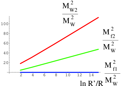
Figure 3: The mass spectrum of fermions and gauge bosons from 6.8 and 5.7 as a function of the warp factor. Here we have chosen $c=-1$ and $a=\frac{1}{10}$, so that $\ln\frac{R^{\prime}}{R}$ grows with $N$. For this plot we used values of $N$ between $20$ and $160$. The bottom curve shows the ratio of the mass squares of the lightest fermion vs. the lightest gauge bosons, confirming that the lightest fermion is essentially massless. The middle curve is the ratio of the mass squares of the next-to-lightest fermion to the lightest gauge boson, confirming that the mass of this fermion increases with the warp factor, and finally the top curve shows the ratio of the mass squares of the next-to-lightest vs. lightest gauge bosons.

7 A Strongly Coupled Scalar Mode

We have seen that by treating the gauge field dynamically in the fifth direction and working in a strongly warped AdS space, the gauge symmetry may be restored in the appropriate limit. In addition, we have shown that the light fermion localized near the IR brane may be given a KK scale mass and decoupled from the theory. This classical construction is then a chiral gauge theory on a lattice, at least in the deconstruction picture we have used so far. In the absence of any large coupling constants we would not expect quantum corrections to bring about qualitative changes to this construction.

However, our construction is based on having an independent gauge group at each slice along the fifth dimension. Furthermore, as has been shown in Section 5, individual groups are strongly coupled in the large $N$ limit. Since the Yukawa couplings of the light fermions to a Goldstone mode of the lightest gauge field are determined by the gauge couplings and the wave-function overlaps, these Yukawa’s may become large.

Indeed, we are forced to introduce a new degree of freedom on every four dimensional lattice which is the radially frozen Higgs or, in the five dimensional language, the fifth component of the gauge field: $A^{5}$. As we show below the angular part of this radially frozen Higgs, which is a would-be Goldstone boson, becomes strongly coupled to the fermions near the IR brane. We might worry that these large Yukawa couplings play the same role as the infinite Yukawa coupling in [23] and push the otherwise massive fermion away from the brane thereby decoupling it from the brane-localized singlets and making it light again. In this section, we calculate these Yukawa couplings and consider some of the possible implications for the wave function of the lightest mode and its mass. We will see that in contrast to [23] (where the large, sudden change in Yukawa coupling was responsible for the modification of the fermion wave-function) the dependence of Yukawa’s on the extra dimensional coordinate in our case will be smooth. Whether this difference suffices to keep all the right handed charged fermions massive will require a lattice calculation, but we proceed with perturbative estimates, which are necessarily qualitative, below.

7.1 Calculation of the Yukawa

We will again make use of the continuum results from Higgsless models in $AdS$. For each KK mode of the gauge field, there is a corresponding Goldstone mode which is eaten to become the massive longitudinal component of the gauge KK mode. Only the Goldstone mode corresponding to the lightest gauge mode is becoming light as the symmetry is restored, so we don’t expect significant effects from the other modes. The coupling of, and mass term for, the gauge field are:

$$g_{5}\int_{R}^{R^{\prime}}dz\left(\frac{R}{z}\right)^{4}A_{\mu}(z)[\psi\sigma^{\mu}\bar{\psi}+\bar{\chi}\bar{\sigma}^{\mu}\chi]+\frac{1}{2}\int_{R}^{R^{\prime}}dz\frac{R}{z}M_{W}^{2}A_{\mu}^{2}\,.$$ (7.1)

As the mass $M_{W}\to 0$, the longitudinal part of the 4D gauge boson behaves like a scalar Goldstone mode, $\phi$, from which it arose:

$$A_{L\mu}(z)\to\frac{f(z)}{M_{W}}\partial_{\mu}\phi\,,$$ (7.2)

where $f(z)$ is the wave function in the extra dimension of the lightest mode of the gauge boson and the normalization is chosen to make the kinetic term of the Goldstone mode canonical. By using the above expressions in the action and integrating by parts with respect to $\partial_{\mu}$, we have:

$$g_{5}\int_{R}^{R^{\prime}}dz\left(\frac{R}{z}\right)^{4}\frac{f(z)\phi}{M_{W}}\partial_{\mu}[\psi\sigma^{\mu}\bar{\psi}+\bar{\chi}\bar{\sigma}^{\mu}\chi]+\frac{1}{2}\int_{R}^{R^{\prime}}dz\frac{R}{z}f^{2}\left(\partial_{\mu}\phi\right)^{2}\,.$$ (7.3)

We can make use of the equations of motion for the fermions, equations (4.12) and (4.13), and integrate by parts again, now with respect to $\partial_{z}$, to get the following form for the action:

$$ig_{5}\int_{R}^{R^{\prime}}dz\left(\frac{R}{z}\right)^{4}\partial_{z}f(z)\frac{\phi}{M_{W}}(\bar{\chi}\bar{\psi}-\psi\chi)+\frac{1}{2}\left(\int_{R}^{R^{\prime}}dz\frac{R}{z}f^{2}\right)\left(\partial_{\mu}\phi\right)^{2}\,.$$ (7.4)

Let us emphasize that the Goldstone mode is a four dimensional degree of freedom with canonical normalization. The expressions for the mass and wave function, to leading order in $\frac{1}{\ln(R^{\prime}/R)}$, are:

$$M_{W}^{2}=\frac{2}{R^{\prime 2}\log\frac{R^{\prime}}{R}},\ \ f(z)=\frac{1}{\sqrt{R\log\frac{R^{\prime}}{R}}}\left(1-\frac{z^{2}\log\frac{z}{R}}{R^{\prime 2}\log\frac{R^{\prime}}{R}}\right)\,.$$ (7.5)

Putting all of it together we get the coupling of the fermions to the Goldstone mode:

$$i\sqrt{2}\frac{g_{5}}{\sqrt{R}}\int_{R}^{R^{\prime}}dz\left(\frac{R}{z}\right)^{4}\phi\frac{z}{R^{\prime}}\frac{\log{\frac{z}{R}}}{\log{\frac{R^{\prime}}{R}}}(\bar{\chi}\bar{\psi}-\psi\chi)\,.$$ (7.6)

If we take into account the fact that the same factor of $\left(\frac{R}{z}\right)^{4}$ appears in the kinetic term, the effective $z$-dependent Yukawa coupling for canonically normalized fields looks like

$$y(z)=\sqrt{2}\,\frac{g_{5}}{\sqrt{R}}\,\frac{z}{R^{\prime}}\,\frac{\log{\frac{z}{R}}}{\log{\frac{R^{\prime}}{R}}}\,.$$ (7.7)

In light of the discussion leading to (5.10), the bare five dimensional gauge coupling is to be evaluated at the cutoff scale, $\frac{1}{Ra}$, but we wish to hold the low energy coupling fixed. From the scaling arguments leading to equation (5.18), the Yukawa coupling becomes

$$y(z)=\frac{4\pi}{\sqrt{b}}\,\frac{z}{R^{\prime}}\,\frac{\log{\frac{z}{R}}}{\log{\frac{R^{\prime}}{R}}}\,.$$ (7.8)

This number, though finite, may be large, so we need to consider how it affects the wave function of the fermion mode which we are trying to remove by using the mass term on the IR brane. It is important to note that (7.8) is substantially different from the result in [23]. There the Yukawa coupling was localized at a single site, and it was possible to do either a perturbative or a strong coupling expansion. Here the Yukawa is smoothly changing in space between zero and a fixed value of order unity so that, in this setup, it is not possible to apply either the weak or strong coupling expansions. A lattice simulation is necessary to really decide whether or not there will be additional light fermions.

7.2 Perturbative Corrections to the Wave Function

We will now make use of this expression for the Yukawa coupling of the fermions to the Goldstone mode to estimate the effect that renormalization has on the wave functions of the fermions. We will look at the regime near the IR brane where the Yukawa is growing large but still perturbative. We will first consider how the fermion operators on each slice, and the operators connecting slices, are renormalized and then use the form of the renormalized parameters to understand the new fermion wavefunction in the fifth direction.

We first rescale the fermion fields to have canonical kinetic terms. The Lagrangian we are now working with is:

$$-i\left(\psi\sigma^{\mu}\partial_{\mu}\bar{\psi}+\bar{\chi}\bar{\sigma}^{\mu}\partial_{\mu}\chi\right)+\psi\partial_{5}\chi-\bar{\chi}\partial_{5}\bar{\psi}+\frac{c}{z}\left(\chi\psi+\bar{\psi}\bar{\chi}\right)$$

$$\qquad+\frac{1}{2}\partial_{\mu}\phi\partial^{\mu}\phi+iy(z)\phi\left(\bar{\psi}\bar{\chi}-\chi\psi\right)\,.$$ (7.9)

The full action should have boundary terms which come about from an integration by parts, but these will not be important for the bulk analysis which we perform here.

Figure 4: The Goldstone exchange contributions. The left graph gives rise to mass and $\partial_{5}$ renomalization while the graph on the right renormalizes the kinetic term.

From evaluation of the diagrams in Fig. 4 we find that in the perturbative regime, the form of the corrected action due to the Yukawa coupling is expected to be

$$-i(1+Ay(z)^{2})\left(\psi\sigma^{\mu}\partial_{\mu}\bar{\psi}+\bar{\chi}\bar{\sigma}^{\mu}\partial_{\mu}\chi\right)+(1+By(z)^{2})\left(\psi\partial_{5}\chi-\bar{\chi}\partial_{5}\bar{\psi}\right)$$

$$+\left(1-By(z)^{2}\right)\frac{c}{z}\left(\chi\psi+\bar{\psi}\bar{\chi}\right)+By(z)^{2}\partial_{z}\ln y(z)(\chi\psi-\bar{\psi}\bar{\chi})\,.$$ (7.10)

The constants $A,B$ would, in perturbation theory, be ${\cal O}(1/16\pi^{2})$. Since perturbation theory is not applicable here we will leave them as undetermined constants of order one.

As stated above, we wish to give a mass of order $1/R^{\prime}$ to the lightest mode of the $\chi$ field (which is localized at the IR brane if $c<-\frac{1}{2}$) by coupling that field to a neutral mode on the IR brane. We can, in principle, give this fermion a site mass of order $1/R^{\prime}$, but wavefunction corrections will suppress or enhance this mass if the mode is pushed away or towards the IR brane. In addition by rescaling the field to get a canonical kinetic term, the effective coupling on the IR brane will be suppressed or enhanced if the four dimensional kinetic term is enhanced or suppressed, respectively.

Taking these considerations into account and making the approximation that the Yukawa coupling is linear in $z$ (dropping the $\log$ dependence), we find the new zero mode wave function:

$$g^{(0)}(z)=N_{0}z^{-c}\left(1+B\frac{16\pi^{2}}{b}\frac{z^{2}}{R^{\prime 2}}\right)^{c-1/2}\,,$$ (7.11)

where $N_{0}$ is a normalization constant. After including the modified kinetic term in the normalization condition, we find that the effective mass term on the IR brane which couples the gauge singlet fermion to our light IR localized mode is

$$\frac{\left(1+\tilde{B}\right)^{c-1/2}}{R^{\prime}\sqrt{\int\frac{d\tilde{z}}{\tilde{z}^{2c}}\left(1+\tilde{A}\tilde{z}^{2}\right)\left(1+\tilde{B}\tilde{z}^{2}\right)^{2c-1}}}\,,$$ (7.12)

where $\tilde{z}=z/R^{\prime}$, $\tilde{A}=A\frac{16\pi^{2}}{b}$ and similarly for $\tilde{B}$. We plot this mass in units of $1/R^{\prime}$ for various values of $\tilde{A}$ and $\tilde{B}$ in Fig. 5.

Figure 5: The mass of the IR localized fermion in units of the KK scale, $1/R^{\prime}$ as a function of $\tilde{B}$ for three values of $\tilde{A}$: $-1$, $3$, $20$ from top to bottom. We have chosen $c=-1$ and performed the integral in (7.12) from $\tilde{z}=0$ to $1$.

For negative values of $\tilde{A}$ or $\tilde{B}$ it is less clear that the perturbative expressions given here can be used to estimate the mass at the IR brane since there is a pole in either the kinetic term or the wave function. Nevertheless, if we take this estimate of the mass seriously even for large values of $\tilde{A}$ and $\tilde{B}$, then the mass of the unwanted fermion is some fixed fraction of the KK mass, $1/R^{\prime}$. In the large $N$ limit, where the KK modes decouple, this fermion will still be removed from the low energy spectrum. Problems may arise, however, if either $\tilde{A}$ or $\tilde{B}$ grow with $N\sim\ln(R^{\prime}/R)$ so that the fermion mass is not a fixed fraction of the KK mass. This may happen if the lattice regularization does not respect the local cutoffs, $v_{n}$, which is a non-trivial issue, as we explain in the next section.

A complete determination of the actual mass of this fermion mode will have to be done using a full non-perturbative lattice computation.

8 Comments on the Full Regularization of the Theory

As discussed in section 4, the warping is a crucial feature of the extra dimension. It is the warp factor which suppresses the mass of the gauge boson below the scale of the KK modes,

$$M_{W}^{2}\sim\frac{m_{KK}^{2}}{\log\frac{R^{\prime}}{R}}\,,$$ (8.1)

which is necessary in order to find a limit which restores the gauge symmetry without making the fermions light. However, this logarithmic suppression of the mass appears to be an inefficient way to approach the symmetric phase and we might hope to do better. In general, a more highly warped background will lead to a larger mass suppression and so we might hope to restore the gauge symmetry more efficiently with a stronger warp factor than that from AdS. Only in AdS, however, do we know of a scaling symmetry which protects the warp factor under renormalization and without a symmetry it is not clear that a stronger warping could be maintained.

Unfortunately a naïve lattice regularization does not respect the scaling symmetry of AdS and will therefore most likely change the wave functions and masses of the modes we are interested in. In particular, if we want to maintain the hypercubic subgroup of the four dimensional Lorentz group, we only find lattices that have an equal spacing, $a_{4}$, in the four flat directions independent of the location in the fifth direction, $z$. For a scalar field the action is:

$$\frac{1}{2}\sum_{i,j}a_{4}^{4}\delta z_{j}\left(\frac{R}{z_{j}}\right)^{5}\left[\left(\frac{z_{j}}{R}\right)^{2}\left(\frac{(\Delta_{4}\phi_{ij})^{2}}{a_{4}^{2}}-\frac{(\Delta_{z}\phi_{ij})^{2}}{\delta z_{j}^{2}}\right)-m^{2}\phi_{ij}^{2}\right]\,,$$ (8.2)

where $i$ represents a general four dimensional index and $j$ represents an index along the fifth dimension. By defining a dimensionless field

$$\tilde{\phi}_{i,j}=a_{4}\sqrt{aR}\,w^{j-1}\phi_{i,j},$$ (8.3)

we may rewrite the action as

$$\frac{1}{2}\sum_{i,j}\left[\left(\Delta_{4}\tilde{\phi}_{i,j}\right)^{2}-\left(\frac{a_{4}}{aR}\right)^{2}w^{2j}\left(\tilde{\phi}_{i,j+1}-(1+a)\tilde{\phi}_{i,j}\right)^{2}-a_{4}^{2}w^{2j-2}m^{2}\tilde{\phi}_{i,j}^{2}\right]\,.$$ (8.4)

We can now see that on the lattice, the mass will still be warping down along the fifth direction. However, it is the four dimensional lattice spacing, $a_{4}$, which sets the scale of the cutoff and that scale is constant. Quantum corrections may therefore destroy the warping of the bulk masses which were necessary to generate a separation of scales between the low energy fermion and gauge boson masses.

Of course, an exact AdS lattice should not be necessary, and it is likely that an appropriate choice of bare parameters would generate an effective action with the properties needed. This mild tuning of the lattice may be the most practical route for constructing a chiral gauge theory. However, if the theory proves difficult to tune, it would be nice to know whether there exists, at least in principle, a regularization which does respect the scaling symmetry of AdS.

We might find a hint of this using higher order derivative operators to regulate the theory. The coefficients of these derivative operators are dimensionful parameters which can be made to respect the scaling symmetry while maintaining the 4D Lorentz invariance. We consider here only a scalar field theory, and the more involved calculation in a gauge theory will need further study.

To understand how the higher derivatives respect the scaling symmetry, we begin by considering operators which are quadratic in the field and have some arbitrary number of derivatives. Schematically, this looks like $\partial_{M}^{n}\phi^{2}$. The indices must be contracted with the metric which brings in one factor of $z/R$ for each derivative. Finally, we must rescale the field to get a canonical four dimensional kinetic term when we are done, $\phi\to\frac{z}{R}\phi$. So we start with

$$\int d^{4}xdz\frac{R}{z}\left(\left(\partial_{M}\phi\right)^{2}+\dots+\frac{\partial_{M}^{n}\phi^{2}}{\left(\frac{R}{z}\Lambda\right)^{n-2}}+\frac{1}{R\Lambda}\frac{\partial_{M}^{n-1}\phi^{2}}{\left(\frac{R}{z}\Lambda\right)^{n-3}}+\dots\right)$$ (8.5)

in our action. The mass scale $\Lambda$ was added to give this higher derivative operator the right mass dimension. The terms with fewer than $n$ derivatives come from $\partial_{z}$ acting on the factor of $z/R$ when the fields are rescaled. Except for the leading factor, the dimensionful scales are warping down the way we want, but we still need to make the $z$ direction discrete. This will bring in one factor of $z/R$ from $dz$, removing the unwanted leading factor and making the four dimensional kinetic operator canonical. Also, the derivatives in the $z$ direction lead to a coupling between adjacent sites with a dimensionful coupling parameter given by

$$\partial_{z}\phi\to\frac{\phi_{j+1}-\phi_{j}}{az_{j}}\,.$$ (8.6)

If we choose the five dimensional cutoff $1/az_{j}$ to be $R\Lambda/z_{j}$ then, indeed, every dimensionful parameter in our deconstructed AdS₅ theory will be warping the way we want. It is known that for scalar interactions, as well as for the nonchiral fermions that we start with, such a regularization renders the theory finite to all orders in perturbation theory, and it can be renormalized in the usual way.

To simulate the theory numerically in the non-perturbative regime, one can put the slices on a four dimensional lattice with uniform $z-$independent spacing $a_{4}$. This will break the scaling symmetry at the lattice scale $1/a_{4}$. A theorem by Reisz [29], however, states that for diagrams with a negative lattice divergence, the continuum limit of the lattice perturbation theory is the same as the continuum perturbation theory. It is easy to see that a naïve discretization of (8.5) belongs to this class. Applying the theorem to the matching between the continuum deconstructed and the lattice regularized theory, one would, therefore, expect that the renormalized theory, at a fixed $\Lambda$, restores the scale invariance as $a_{4}\to 0$; and taking $\Lambda\to\infty$ holding $a_{4}\Lambda=0$ then recovers the original scale-invariant lattice theory.

9 Consistency with Anomalies and Instantons

So far we have not discussed gauge anomalies, however if we tried to perform our procedure in such a way so as to leave an anomalous light fermion content, then loop corrections would produce a mass for the gauge boson that is not removed in the small curvature radius limit. This effect is well known [30]: two back to back triangle anomalies produce a gauge boson mass at order $g^{3}$. It is this effect that shows that an anomalous gauge theory with an unbroken gauge symmetry is not a consistent possibility, and thus it is to be expected that this same effect is what prevents the procedure described in this paper from constructing an anomalous unbroken gauge theory.

A consistent latticization of a chiral gauge theory should also make clear how the instantons of the low energy chiral gauge theory are produced. In fact, the chiral fermion measure is complex, and its phase depends on the gauge field configuration in a non-trivial way leading to the non-conservation of individual fermion currents in an instanton background. This is a non-trivial question since the ’t Hooft operator generated by the instanton of a single chiral theory contains only left handed fields, while the individual instantons in every gauge group would generate a ’t Hooft operator with equal number of left and right handed fermions. In the absence of a Majorana mass for the gauge singlet fermions one can, in fact, reproduce neither the phase of fermion measure, nor such non-perturbative effects of the chiral gauge theory, since the Dirac measures we start with are real and there is no way to flip the chiralities. This is in accordance with the observation that the spectrum from (6.8) will be chiral only for $m_{M}\neq 0$. For $m_{M}\neq 0$, however, one can chain together several instantons such that the right handed fermions sticking out from the instanton are all transforming under the last gauge group, where the gauge symmetry is broken. At that site the right handed fermions mix with the gauge singlet fermions via the Higgs VEV. These gauge singlet fermions in turn have Majorana masses which can flip the chiralities, thus all legs of right handed fermions can be closed up this way.

As a concrete example, consider constructing a chiral $SU(5)$ gauge theory with a left-handed ${\bf\bar{5}}$ and ${\bf 10}$ fields. With a sufficient number of singlet fermions and Higges we can make heavy all the components of the right-handed ${\bf\bar{5}}$ and ${\bf 10}$ at the final lattice site. Then we see that although we started with a vector-like theory where there are seperately conserved currents for ${\bf\bar{5}}$’s and ${\bf 10}$’s, the chain of instantons and mixing with Majorana singlets reduces the global symmetry, and a current of ${\bf\bar{5}}$’s can be turned into a current of ${\bf 10}$’s. This is illustrated in Fig. 6 where we show how a bunch of $SU(5)$ instantons can be chained together to generate the ’t Hooft operator of a single chiral $SU(5)$ theory.

Figure 6: A chain of instantons in the extra dimension in an $SU(5)$ theory with ${\bf\bar{5},10}$. Arrows represent the chirality of the fermion field, with left handed fermions going into the instanton, and right handed coming out. A Dirac mass connects a left and a right handed fermion so the flow of the arrow will be continuous, while a Majorana mass reverses the direction of the arrow, since it connects two left or two right handed fields. Note, that there are three zero modes for a ${\bf 10}$ field, so the ’t Hooft operator is ${\bf 10}^{3}{\bf\bar{5}}$ (see [31] for details).

10 Conclusions

We have considered the domain wall fermion construction of chiral gauge theories in the presence of non-vanishing curvature in the extra dimension. In the discretized theory without scalar VEV’s there are two light fermions localized at opposite ends of the extra dimension, and the theory is non-chiral. The main new feature of these models is that one can restore gauge invariance in the presence of scalar VEV’s on the IR brane by taking the limit of small curvature radius. Then this scalar VEV can be used to remove one of the two fermion chiralities from the theory. We have checked numerically that the classical theory will indeed result in a chiral gauge theory. The chiral instanton operator can also be reproduced in this model. The main worry is that in the limit of small curvature radius, one light scalar becomes strongly coupled near the IR brane. This could potentially result in additional light fermions. In order to find out whether or not the theory is indeed chiral at the non-perturbative level, a full lattice simulation needs to be performed.

References

- [1] P. V. D. Swift, Phys. Lett. B 145, 256 (1984) ; S. Aoki, I. H. Lee, S. S.Xue, Phys. Lett. B 229, 79 (1989) ; I. Montvay, Phys. Lett. B 199, 89 (1987) ; ibid. B 205, 315 (1988) .
- [2] H. B. Nielsen and M. Ninomiya, Nucl. Phys. B 185, 20 (1981) ; erratum ibid. B 195, 541 (1982) .
- [3] P. H. Ginsparg and K. G. Wilson, Phys. Rev. D 25, 2649 (1982) .
- [4] H. Neuberger, Phys. Lett. B 417, 141 (1998) [arXiv:hep-lat/9707022]; ibid. B 427, 353 (1998) [arXiv:hep-lat/9801031]; P. Hasenfratz, V. Laliena and F. Niedermayer, Phys. Lett. B 427, 125 (1998) [arXiv:hep-lat/9801021].
- [5] M. Lüscher, Phys. Lett. B 428, 342 (1998) [arXiv:hep-lat/9802011].
- [6] M. Lüscher, JHEP 0006, 028 (2000) [arXiv:hep-lat/0006014]; R. Narayanan and H. Neuberger, Phys. Rev. Lett. 71, 3251 (1993) [arXiv:hep-lat/9308011]; H. Neuberger, Phys. Rev. D 63, 014503 (2001) [arXiv:hep-lat/0002032]; S. Ranjbar-Daemi and J. Strathdee, Nucl. Phys. B 443, 386 (1995) [arXiv:hep-lat/9501027].
- [7] A. Borelli, L. Maiani, G. C. Rossi, R. Sisto, and M. Testa, Phys. Lett. B 221, 360 (1989) ; Nucl. Phys. B 333, 335 (1990) .
- [8] G. ’t Hooft, Phys. Lett. B 349, 491 (1998) [arXiv:hep-th/9411228]; P. Hernandez, R. Sundrum, Nucl. Phys. B 455, 287 (1995) [arXiv:hep-ph/9506331]; M. Golterman and Y. Shamir, Phys. Rev. D 70, 094506 (2004) [arXiv:hep-lat/0404011].
- [9] D. B. Kaplan, Phys. Lett. B 288, 342 (1992) [arXiv:hep-lat/9206013].
- [10] M. F. L. Golterman, K. Jansen, D. N. Petcher and J. C. Vink, Phys. Rev. D 49, 1606 (1994) [arXiv:hep-lat/9309015]; M. Golterman, K. Jansen, D. Petcher and J. C. Vink, Nucl. Phys. Proc. Suppl. 34, 593 (1994) [arXiv:hep-lat/9312005].
- [11] L. Randall and R. Sundrum, Phys. Rev. Lett. 83, 4690 (1999) [arXiv:hep-th/9906064]; Phys. Rev. Lett. 83, 3370 (1999) [arXiv:hep-ph/9905221].
- [12] C. Csáki, C. Grojean, H. Murayama, L. Pilo and J. Terning, Phys. Rev. D 69, 055006 (2004) [arXiv:hep-ph/0305237].
- [13] C. Csáki, C. Grojean, L. Pilo and J. Terning, Phys. Rev. Lett. 92, 101802 (2004) [arXiv:hep-ph/0308038].
- [14] Y. Nomura, JHEP 0311, 050 (2003) [arXiv:hep-ph/0309189]; R. Barbieri, A. Pomarol and R. Rattazzi, Phys. Lett. B 591, 141 (2004) [arXiv:hep-ph/0310285].
- [15] R. Sekhar Chivukula, D. A. Dicus and H. J. He, Phys. Lett. B 525, 175 (2002) [arXiv:hep-ph/0111016]; R. S. Chivukula and H. J. He, Phys. Lett. B 532, 121 (2002) [arXiv:hep-ph/0201164]; R. S. Chivukula, D. A. Dicus, H. J. He and S. Nandi, Phys. Lett. B 562, 109 (2003) [arXiv:hep-ph/0302263]; S. De Curtis, D. Dominici and J. R. Pelaez, Phys. Lett. B 554, 164 (2003) [arXiv:hep-ph/0211353]; Phys. Rev. D 67, 076010 (2003) [arXiv:hep-ph/0301059]; Y. Abe, N. Haba, Y. Higashide, K. Kobayashi and M. Matsunaga, Prog. Theor. Phys. 109, 831 (2003) [arXiv:hep-th/0302115].
- [16] T. Gherghetta and A. Pomarol, Nucl. Phys. B 586, 141 (2000) [arXiv:hep-ph/0003129]. H. Georgi, A. K. Grant and G. Hailu, Phys. Rev. D 63, 064027 (2001) [arXiv:hep-ph/0007350]. B. Grzadkowski and M. Toharia, Nucl. Phys. B 686, 165 (2004) [arXiv:hep-ph/0401108].
- [17] N. Arkani-Hamed and M. Schmaltz, Phys. Rev. D 61, 033005 (2000) [arXiv:hep-ph/9903417].
- [18] N. Arkani-Hamed, A. G. Cohen and H. Georgi, Phys. Rev. Lett. 86, 4757 (2001) [arXiv:hep-th/0104005]; C. T. Hill, S. Pokorski and J. Wang, Phys. Rev. D 64, 105005 (2001) [arXiv:hep-th/0104035].
- [19] D. B. Kaplan, E. Katz and M. Unsal, JHEP 0305, 037 (2003) [arXiv:hep-lat/0206019]; A. G. Cohen, D. B. Kaplan, E. Katz and M. Unsal, JHEP 0308, 024 (2003) [arXiv:hep-lat/0302017]; JHEP 0312, 031 (2003) [arXiv:hep-lat/0307012];
- [20] J. Giedt, E. Poppitz and M. Rozali, JHEP 0303, 035 (2003) [arXiv:hep-th/0301048]; J. Giedt and E. Poppitz, JHEP 0409, 029 (2004) [arXiv:hep-th/0407135]; J. Giedt, R. Koniuk, E. Poppitz and T. Yavin, JHEP 0412, 033 (2004) [arXiv:hep-lat/0410041].
- [21] D. E. Kaplan and T. M. P. Tait, JHEP 0111, 051 (2001) [arXiv:hep-ph/0110126].
- [22] W. Skiba and D. Smith, Phys. Rev. D 65, 095002 (2002) [arXiv:hep-ph/0201056].
- [23] M. F. L. Golterman and Y. Shamir, Phys. Rev. D 51, 3026 (1995) [arXiv:hep-lat/9409013].
- [24] S. J. Huber and Q. Shafi, Phys. Rev. D 63, 045010 (2001) [arXiv:hep-ph/0005286].
- [25] Y. Grossman and M. Neubert, Phys. Lett. B 474, 361 (2000) [arXiv:hep-ph/9912408]; T. Gherghetta and A. Pomarol, Nucl. Phys. B 586, 141 (2000) [arXiv:hep-ph/0003129]; S. J. Huber and Q. Shafi, Phys. Lett. B 498, 256 (2001) [arXiv:hep-ph/0010195].
- [26] C. Csáki, C. Grojean, J. Hubisz, Y. Shirman and J. Terning, Phys. Rev. D 70, 015012 (2004) [arXiv:hep-ph/0310355].
- [27] L. Randall, Y. Shadmi and N. Weiner, JHEP 0301, 055 (2003) [arXiv:hep-th/0208120]; A. Falkowski and H. D. Kim, JHEP 0208, 052 (2002) [arXiv:hep-ph/0208058].
- [28] A. Katz and Y. Shadmi, JHEP 0411, 060 (2004) [arXiv:hep-th/0409223].
- [29] T. Reisz, Commun. Math. Phys. 116, 81 (1988); Commun. Math. Phys. 117, 79 (1988).
- [30] J. Preskill, Annals Phys. 210, 323 (1991) .
- [31] C. Csáki and H. Murayama, Nucl. Phys. B 532, 498 (1998) [arXiv:hep-th/9804061].