Finite Volume Dependence of Hadron Properties and Lattice QCD

Abstract

Because the time needed for a simulation in lattice QCD varies at a rate exceeding the fourth power of the lattice size, it is important to understand how small one can make a lattice without altering the physics beyond recognition. It is common to use a rule of thumb that the pion mass times the lattice size should be greater than (ideally much greater than) four (i.e., $m_{\pi}L\gg 4$). By considering a relatively simple chiral quark model we are led to suggest that a more realistic constraint would be $m_{\pi}(L-2R)\gg 4$, where $R$ is the radius of the confinement region, which for these purposes could be taken to be around 0.8-1.0 fm. Within the model we demonstrate that violating the second condition can lead to unphysical behaviour of hadronic properties as a function of pion mass. In particular, the axial charge of the nucleon is found to decrease quite rapidly as the chiral limit is approached.

1 Introduction

Our current capacity to compute hadron properties in lattice QCD is constrained by the need to take many limits. For example, we need to take the spacing $a\rightarrow 0$, the size of the lattice $L\rightarrow\infty$ and the quark mass to around 5 MeV. Of course, these limits are not unconnected because the size of a region of space big enough to contain (say) a proton will need to grow with the Compton wavelength of the pion. At present, with lattice spacings that represent a reasonable approximation to the continuum limit and for full QCD with reasonable chiral symmetry, the time for a lattice simulation scales roughly like $m_{\pi}^{-9}$ and we are limited to pion masses larger than 0.4-0.5 GeV. This has led to much effort to explore the application of chiral perturbation theory as a tool for extrapolating hadron properties to the physical pion mass [1, 2, 3].

In such an environment there is great interest in seeing whether one can lower the pion mass without increasing the size of the lattice, thereby saving a factor of $m_{\pi}^{4}$. Indeed, there have been many calculations for which even the rather optimistic rule of thumb that $m_{\pi}L>4$ has not been satisfied. Considerable attention has been devoted to studying such systems within the framework of effective field theory in order to understand how the relevant path integral might change as we go from one regime to another [4, 5].

The question we ask is somewhat different. We consider a simple chiral quark model upon which we impose boundary conditions which roughly approximate those on a lattice. Simple inspection of the solutions naturally leads one to conclude that the condition noted above is incorrect. Indeed, the pion cloud of the nucleon does not even begin until one is outside the region of space in which the valence quarks are confined. Within the bag model this is characterised by the bag radius, $R$, and within the cloudy bag model as well as the model considered here, this radius is where the pion field peaks. The asymptotic behaviour of the pion field is therefore $\phi(r)\sim exp[-m_{\pi}(r-R)]/r^{2}$ and the correct condition for the pion field to be small on a spherical boundary surrounding the nucleon is that $(L/2-R)\gg m_{\pi}^{-1}$, with $L$ the diameter of the spherical ”lattice”. (Note that in sects. 2 and 3 we will use $L$ to denote the radius of such a region.)

If we consider a typical case where the pion mass is large, say $m_{\pi}=600$ MeV, then on a 2 fm lattice $m_{\pi}L\sim 6$ and the commonly quoted condition would suggest that we had a sufficiently large lattice. However, with a bag radius of order 0.8 fm, we find $m_{\pi}(L/2-R)\sim 0.6$ and the pion field has no chance to drop to zero before we reach the edge of the lattice! Indeed, even at this relatively large mass a 3 fm lattice would be a minimal requirement for full QCD simulations. From the mathematical point of view, having the boundary too close means that we are not restricted to the well behaved solution of the second order differential equation but can have a significant coefficient for the divergent solution. Through the coupling to the confined valence quarks this can in turn change the internal valence structure of the hadron.

Considerations such as these help us to understand why some hadronic properties exhibit a dramatic volume dependence as the pion mass is varied. Perhaps the most famous example is the axial charge of the nucleon where early simulations revealed a striking decrease of $g_{A}$ as the pion mass decreased — in the opposite direction from the experimental data [6, 7, 8]. We shall see that our simple chiral model is able to reproduce this feature.

2 A Simple Chiral Quark Model

One of the earliest attempts to restore chiral symmetry to the MIT bag model was made in 1975 by Chodos and Thorn [9]. Their solution, a precursor to the CBM [10, 11] was a straight forward generalization of the linear sigma model, with pion and sigma fields coupling linearly to the confined quarks at the bag boundary. As well as presenting a perturbative solution in the pion field (as in the CBM), Chodos and Thorn attempted to find an exact solution to the resulting equations of motion. The only case where this was feasible was for a highly idealized baryon called the “hedgehog”, in which the 3 confined quarks all inhabit the same mixed spin-flavour singlet, and which hence is not an eigenstate of either isospin or angular momentum. As a result, the hedgehog solution does not correspond to any physical particle. Despite this fact, the hedgehog approximation does provide a simple classical solution with which we can then study a number of phenomena with relative ease.

Chodos and Thorn suggest the following chirally invariant Lagrangian density based on the MIT bag model Lagrangian:

$${\cal L}_{\scriptscriptstyle\mathit{CT}}=[\bar{\psi}i\partial\!\!\!/\psi-B]\theta_{V}-\lambda\bar{\psi}(\sigma+i\mbox{$\vec{\tau}\cdot\vec{\pi}$}\gamma_{5})\psi\,\delta_{S}+\frac{1}{2}(\partial_{\mu}\sigma)(\partial^{\mu}\sigma)+\frac{1}{2}(\partial_{\mu}\mbox{$\vec{\pi}$})\cdot(\partial^{\mu}\mbox{$\vec{\pi}$}),$$ (1)

where $\psi$, $\vec{\pi}$ and $\sigma$ are the quark, pion and sigma fields, respectively, and $\lambda$ is a Lagrange multiplier which turns out to be $\mbox{$\scriptstyle\frac{1}{2}$}(\sigma^{2}+\pi^{2})^{-1/2}$. This is invariant under the appropriate infinitesimal chiral transformation and the corresponding axial current:

$$\vec{A}^{\mu}=\frac{1}{2}\bar{\psi}\vec{\tau}\gamma_{5}\gamma^{\mu}\psi\theta_{V}+(\partial^{\mu}\sigma)\mbox{$\vec{\pi}$}-\sigma(\partial^{\mu}\mbox{$\vec{\pi}$}),$$ (2)

is conserved.

To this Lagrangian we will also add explicit chiral symmetry breaking quark and pion mass terms. To generate a pion mass we could follow the method of the linear sigma model, spontaneously breaking chiral symmetry and then tipping the Mexican hat potential, generating masses for both the $\vec{\pi}$ and $\sigma$ fields. However, this process leads to some very complex equations of motion for the pion and sigma fields, destroying the simplicity of Chodos and Thorn’s classical solution. For simplicity we include the pion mass (and the corresponding quark mass) by hand, leaving the $\sigma$ field massless. The resulting Lagrangian is

$${\cal L} = [\bar{\psi}(i\partial\!\!\!/-m_{q})\psi-B]\theta_{V}-\lambda\bar{\psi}(\sigma+i\mbox{$\vec{\tau}\cdot\vec{\pi}$}\gamma_{5})\psi\,\delta_{S}$$ (3)

$$+\frac{1}{2}(\partial_{\mu}\sigma)(\partial^{\mu}\sigma)+\frac{1}{2}(\partial_{\mu}\mbox{$\vec{\pi}$})\cdot(\partial^{\mu}\mbox{$\vec{\pi}$})-\frac{1}{2}m_{\scriptscriptstyle\pi}^{2}\mbox{$\vec{\pi}$}\cdot\mbox{$\vec{\pi}$}.$$

Minimizing the action leads to five Euler-Lagrange equations. For a static spherical bag of radius $R$ and static $\sigma$ and $\vec{\pi}$ fields they are as follows:

$$(i\partial\!\!\!/-m_{q})\psi=0, r\leq R;$$ (4)

$$i\hat{r}\cdot\vec{\gamma}\psi=-\xi(\sigma+i\vec{\tau}\cdot\mbox{$\vec{\pi}$}\gamma_{5})\psi, r=R;$$ (5)

$$\nabla^{2}\sigma=\frac{1}{2}\xi\bar{\psi}\psi\,\delta(r-R);$$ (6)

$$\nabla^{2}\mbox{$\vec{\pi}$}-m_{\scriptscriptstyle\pi}^{2}\mbox{$\vec{\pi}$}=\frac{1}{2}\xi\bar{\psi}i\vec{\tau}\gamma_{5}\psi\,\delta(r-R);$$ (7)

$$B=-\frac{1}{2}\xi\frac{\partial}{\partial r}\bigl{[}\bar{\psi}(\sigma+i\mbox{$\vec{\tau}\cdot\vec{\pi}$}\gamma_{5})\psi\bigr{]}_{r=R,}$$ (8)

where we use the notation $\xi=[\sigma^{2}(R)+\pi^{2}(R)]^{-1/2}$. The first of these equations is just the Dirac equation for the confined quarks, whilst Eqs. (6) and (7) are equations of motion for the sigma and pion fields. There are also two boundary conditions — the linear boundary condition, Eq. (5), and the non-linear boundary condition, Eq. (8), with similar roles to their roles in the MIT model.

Chodos and Thorn solve this system of equations (without quark and pion masses) on an infinite volume. Following their method, we will solve the system on a finite spherical volume of radius $L$. Ideally we would use a rectangular volume similar to that used in lattice simulations but because of the radial nature of the solutions it is natural to use a spherical volume and any attempt to solve on a rectangular volume would be significantly more complicated.

The quark field solution is just the MIT quark wavefunction,

$$\psi(\vec{r},t)=\mbox{$\left(\begin{array}[]{c}\displaystyle\alpha_{\scriptscriptstyle+}j_{0}\bigl{(}\frac{\Omega r}{R}\bigr{)}\\ \displaystyle i\alpha_{\scriptscriptstyle-}j_{1}\bigl{(}\frac{\Omega r}{R}\bigr{)}\,\vec{\sigma}\cdot\hat{r}\end{array}\right)$ }\chi_{\scriptscriptstyle h}\,\theta(R-r)\,e^{-i\alpha t/R},$$ (9)

where we define $\alpha=ER$ and $\Omega=kR$ (where $k$ is to be determined by the appropriate eigenvalue condition) related by the equation

$$\alpha=\sqrt{\Omega^{2}+(m_{q}R)^{2}},$$ (10)

and

$$\alpha_{\scriptscriptstyle\pm}=\sqrt{\frac{\alpha\pm m_{q}R}{\alpha}}.$$ (11)

The defining property of the hedgehog solution is the choice of static, radially dependent sigma and pion fields,

$$\mbox{$\vec{\pi}$}(\vec{r}) = g(r)\hat{r},$$ (12)

$$\sigma(\vec{r}) = f(r),$$ (13)

and the choice of spinor-isospinor, $\chi_{\scriptscriptstyle h}$, proportional to a mixed spin-isospin singlet state,

$$\hat{\chi_{\scriptscriptstyle h}}=\frac{1}{\sqrt{2}}\bigl{(}|d\uparrow\rangle-|u\downarrow\rangle\bigr{)},$$ (14)

so that it has the property,

$$(\vec{\sigma}+\vec{\tau})\chi_{\scriptscriptstyle h}=0.$$ (15)

These choices greatly simplify the equation for the pion field by ensuring that $\bar{\psi}\vec{\tau}\gamma_{5}\psi$ is proportional to $\hat{r}$ and hence to $\vec{\pi}$:

$$\bar{\psi}\vec{\tau}\gamma_{5}\psi=-2i\,j_{0}j_{1}\,\chi_{\scriptscriptstyle h}^{\dagger}\chi_{\scriptscriptstyle h}\,\hat{r}.$$ (16)

Substituting Eqs. (9), (12) and (13) into the equations of motion for $\vec{\pi}$ and $\sigma$, yields the following two second order differential equations in $f$ and $g$:

$$f^{\prime\prime}(r)+\frac{2}{r}f^{\prime}(r) = \frac{1}{2}\xi\bigl{(}\alpha_{\scriptscriptstyle+}^{2}j_{0}^{2}(\Omega)-\alpha_{\scriptscriptstyle-}^{2}j_{1}^{2}(\Omega)\bigr{)}\chi_{\scriptscriptstyle h}^{\dagger}\chi_{\scriptscriptstyle h}\,\delta(R-r)$$ (17)

$$\equiv a\,\delta(R-r),$$

$$g^{\prime\prime}(r)+\frac{2}{r}g^{\prime}(r)-\bigl{(}\frac{2}{r^{2}}+m_{\scriptscriptstyle\pi}^{2}\bigr{)}g(r) = \xi\alpha_{\scriptscriptstyle+}\alpha_{\scriptscriptstyle-}j_{0}(\Omega)j_{1}(\Omega)\chi_{\scriptscriptstyle h}^{\dagger}\chi_{\scriptscriptstyle h}\,\delta(R-r)$$ (18)

$$\equiv b\,\delta(R-r).$$

Enforcing regularity at the origin, Eqs. (17) and (18) have solutions

$$f(r) = f_{0}+aR^{2}\bigl{(}\frac{1}{R}-\frac{1}{r}\bigr{)}\theta(r-R),$$ (19)

$$g(r) = \bigl{(}-\frac{\cosh rm_{\scriptscriptstyle\pi}}{rm_{\scriptscriptstyle\pi}}+\frac{\sinh rm_{\scriptscriptstyle\pi}}{r^{2}m_{\scriptscriptstyle\pi}^{2}}\bigr{)}\Bigl{[}C+b\bigl{(}R\sinh Rm_{\scriptscriptstyle\pi}-\frac{\cosh Rm_{\scriptscriptstyle\pi}}{m_{\scriptscriptstyle\pi}}\bigr{)}\theta(r-R)\Bigr{]}+$$ (20)

$$\bigl{(}\frac{\sinh rm_{\scriptscriptstyle\pi}}{rm_{\scriptscriptstyle\pi}}-\frac{\cosh rm_{\scriptscriptstyle\pi}}{r^{2}m_{\scriptscriptstyle\pi}^{2}}\bigr{)}b\bigl{(}R\cosh Rm_{\scriptscriptstyle\pi}-\frac{\sinh Rm_{\scriptscriptstyle\pi}}{m_{\scriptscriptstyle\pi}}\bigr{)}\theta(r-R),$$

where $f_{0}$ and $C$ are constants of integration.

At the boundary $r=L$ we set the derivative $\vec{\pi}^{\prime}$ to zero to resemble the periodic boundary conditions applied in lattice simulations. We stress that in this context $L$ is not the lattice length, which would be of order $2L$. Because there is no sigma mass we cannot enforce a similar condition on $\sigma$. Instead we leave $f_{0}$ as a free parameter for the moment. The resulting solutions are

$$f(r) = f_{0}+aR^{2}(\frac{1}{R}-\frac{1}{r})\theta(r-R),$$ (21)

$$g(r) = b\bigl{(}R\cosh Rm_{\scriptscriptstyle\pi}-\frac{\sinh Rm_{\scriptscriptstyle\pi}}{m_{\scriptscriptstyle\pi}}\bigr{)}\bigl{(}\frac{\sinh rm_{\scriptscriptstyle\pi}}{rm_{\scriptscriptstyle\pi}}-\frac{\cosh rm_{\scriptscriptstyle\pi}}{r^{2}m_{\scriptscriptstyle\pi}^{2}}\bigr{)}\theta(r-R)+$$ (22)

$$b\bigl{(}R\sinh Rm_{\scriptscriptstyle\pi}-\frac{\cosh Rm_{\scriptscriptstyle\pi}}{m_{\scriptscriptstyle\pi}}\bigr{)}\bigl{(}\frac{\cosh rm_{\scriptscriptstyle\pi}}{rm_{\scriptscriptstyle\pi}}-\frac{\sinh rm_{\scriptscriptstyle\pi}}{r^{2}m_{\scriptscriptstyle\pi}^{2}}\bigr{)}\theta(R-r)+$$

$$b\bigl{(}R\cosh Rm_{\scriptscriptstyle\pi}-\frac{\sinh Rm_{\scriptscriptstyle\pi}}{m_{\scriptscriptstyle\pi}}\bigr{)}\bigl{(}-\frac{\cosh rm_{\scriptscriptstyle\pi}}{rm_{\scriptscriptstyle\pi}}+\frac{\sinh rm_{\scriptscriptstyle\pi}}{r^{2}m_{\scriptscriptstyle\pi}^{2}}\bigr{)}\Gamma(Lm_{\scriptscriptstyle\pi}),$$

where the $L$-dependence is given by the function,

$$\Gamma(Lm_{\scriptscriptstyle\pi})=\biggl{(}\frac{\frac{\cosh Lm_{\scriptscriptstyle\pi}}{Lm_{\scriptscriptstyle\pi}}-2\frac{\sinh Lm_{\scriptscriptstyle\pi}}{L^{2}m_{\scriptscriptstyle\pi}^{2}}+2\frac{\cosh Lm_{\scriptscriptstyle\pi}}{L^{3}m_{\scriptscriptstyle\pi}^{3}}}{\frac{\sinh Lm_{\scriptscriptstyle\pi}}{Lm_{\scriptscriptstyle\pi}}-2\frac{\cosh Lm_{\scriptscriptstyle\pi}}{L^{2}m_{\scriptscriptstyle\pi}^{2}}+2\frac{\sinh Lm_{\scriptscriptstyle\pi}}{L^{3}m_{\scriptscriptstyle\pi}^{3}}}\biggr{)}.$$ (23)

(Note that $\Gamma(Lm_{\scriptscriptstyle\pi})\to 1$ as $L\to\infty$).

2.1 The linear boundary condition

The solutions to Eqs. (4), (6) and (7) are dependent on the parameters $\Omega$, $R$, $L$, $m_{q}$ and $m_{\scriptscriptstyle\pi}$ but also on the unknown values $f(R)$ and $g(R)\equiv g_{0}$, which are given by

$$f(R) = f_{0},$$ (24)

$$g(R) = -\xi\alpha_{\scriptscriptstyle+}\alpha_{\scriptscriptstyle-}j_{0}j_{1}\chi_{\scriptscriptstyle h}^{\dagger}\chi_{\scriptscriptstyle h}\bigl{(}R\cosh Rm_{\scriptscriptstyle\pi}-\frac{\sinh Rm_{\scriptscriptstyle\pi}}{m_{\scriptscriptstyle\pi}}\bigr{)}\times$$ (25)

$$\Bigl{[}\bigl{(}-\frac{\sinh Rm_{\scriptscriptstyle\pi}}{Rm_{\scriptscriptstyle\pi}}+\frac{\cosh Rm_{\scriptscriptstyle\pi}}{R^{2}m_{\scriptscriptstyle\pi}^{2}}\bigr{)}+\bigl{(}\frac{\cosh Rm_{\scriptscriptstyle\pi}}{Rm_{\scriptscriptstyle\pi}}-\frac{\sinh Rm_{\scriptscriptstyle\pi}}{R^{2}m_{\scriptscriptstyle\pi}^{2}}\bigr{)}\Gamma(Lm_{\scriptscriptstyle\pi})\Bigr{]}$$

$$\equiv -\xi\,d(\Omega,m_{q},m_{\scriptscriptstyle\pi},R,L).$$ (26)

If we now apply the linear boundary condition, Eq. (5), we may express $f_{0}^{2}$, $g_{0}^{2}$ and $1/\xi^{2}$ in terms of $y$ and $d$:

$$f_{0}^{2}=\frac{4y^{2}}{1-y^{4}}\,d,\hskip 28.45274ptg_{0}^{2}=\frac{1-y^{2}}{1+y^{2}}\,d,\hskip 28.45274pt\frac{1}{\xi^{2}}=\frac{1+y^{2}}{1-y^{2}}\,d,$$ (27)

so that our solution now depends only on the parameters $\Omega$, $m_{q}$, $m_{\scriptscriptstyle\pi}$, $R$ and $L$.

2.2 The non-linear boundary condition

The last condition to apply is the non-linear boundary condition, Eq. (8), which sets the bag energy density $B$. Because of the discontinuity in the derivatives of the $\vec{\pi}$ and $\sigma$ fields at the bag boundary, $r=R$, we take the average of the derivative on each side, that is:

$$\frac{\partial\sigma}{\partial r}\Bigr{|}_{r=R}\equiv\frac{1}{2}\Bigl{(}\frac{\partial\sigma^{(in)}}{\partial r}+\frac{\partial\sigma^{(out)}}{\partial r}\Bigr{)}\Bigr{|}_{r=R}.$$ (28)

With the solutions for $\psi$, $\vec{\pi}$ and $\sigma$, Eq. (8) leads to an expression for $B$ of the form,

$$4\pi R^{4}B=\tau(\Omega,m_{q},m_{\scriptscriptstyle\pi},R,L),$$ (29)

where $\tau$ is a complicated function of the bag frequency $\Omega$, hedgehog and volume radii ($R$ and $L$ respectively), and quark and pion masses. Because of its complexity, the explicit form of $\tau$ and the involved steps required to find it are not shown.

Once the masses and volume size are set, Eq. (29) becomes a three-way relationship between the parameters $B$, $R$ and $\Omega$. By choosing a value for the bag energy density (a property of the vacuum) the radius $R$, and hence the entire solution, will be completely determined by $\Omega$. Using this fact we can now find an eigenvalue condition for $\Omega$. Using the linear and non-linear boundary conditions, we find that the value of the sigma field at the boundary $r=L$,

$$\sigma(L)=f(L)=f_{0}+aR^{2}\bigl{(}\frac{1}{R}-\frac{1}{L}\bigr{)},$$ (30)

is completely specified by the energy parameter $\Omega$. Fig. 1 shows a plot of $1/f(L)^{2}$ against $\Omega$ for fixed parameters $B$, $m_{q}$, $m_{\scriptscriptstyle\pi}$ and $L$.

Figure 1: Plot of the inverse square of the value of the sigma field at the boundary $r=L$ versus the bag frequency $\Omega$. The horizontal line represents the boundary condition $f(L)=f_{\scriptscriptstyle\pi}$.

Physical solutions occur for $\Omega$ within specific allowed regions or bands. Outside of these regions either $\sigma^{2}$ is negative and hence $\sigma$ is imaginary, or $\tau(\Omega)$ is negative, in which case there are no real solutions to the n.l.b.c. By selecting a boundary condition for the sigma field (represented by a horizontal line in Fig. 1) we can find eigenvalues of the bag frequency, $\Omega$. From Fig. 1 we see that $1/f(L)^{2}$ has a limited size so there is a limit to how small we can make $\sigma(L)$.

So what boundary condition should we apply to $\sigma$? Starting with the PCAC relation

$$\bigl{\langle}0\bigr{|}\partial_{\mu}A_{a}^{\mu}(x)\bigl{|}\pi_{b}(q)\bigr{\rangle}=f_{\scriptscriptstyle\pi}m_{\scriptscriptstyle\pi}^{2}\,\delta_{ab}\,e^{-iq\cdot x}\,,$$ (31)

we substitute the axial current of Eq. (2) into the left-hand side and take the limit $r\to\infty$ (where $\psi=0$) then we find

$$\bigl{\langle}0\bigr{|}\partial_{\mu}A_{a}^{\mu}(x)\bigl{|}\pi_{b}(q)\bigr{\rangle} = \bigl{\langle}0\bigr{|}\bigl{\{}(\partial^{2}\sigma)\pi_{a}-\sigma(\partial^{2}\pi_{a})\bigr{\}}\bigl{|}\pi_{b}(q)\bigr{\rangle}$$ (32)

$$= m_{\scriptscriptstyle\pi}^{2}\mbox{$\langle\sigma\rangle$}\delta_{ab}\,e^{-iq\cdot x}\,.$$ (33)

Comparing with Eq. (31), we see that the vacuum expectation value of the sigma field must be $\mbox{$\langle\sigma\rangle$}=f_{\scriptscriptstyle\pi}$ so we expect the sigma field to go to $f_{\scriptscriptstyle\pi}$ at infinity.

To find the hedgehog solution on an infinite volume we would therefore choose $f_{0}$ such that $f(r)\to f_{\scriptscriptstyle\pi}$ as $r\to\infty$. For large volumes, setting $f(L)=f_{\scriptscriptstyle\pi}$ should still be an appropriate boundary condition. But for smaller volumes this is too harsh a condition and is found to introduce large volume dependence. As an alternative, we fix the sigma field at $r=L$ to the value taken by $\sigma(L)$ in the infinite volume solution (in which $\sigma\to f_{\scriptscriptstyle\pi}$ as $r\to\infty$). This results in a more modest volume dependence, which seems appropriate given that in non-linear chiral models the sigma mass is usually set to infinity and we expect volume dependence to arise mainly from the effect of the $\vec{\pi}$ field.

Figure 2: The quark density $\psi^{\dagger}\psi$ (full line) and magnitudes of the pion (dashed line) and sigma (dotted line) fields in the hedgehog solution calculated at the physical pion mass on a spherical volume of radius $L=100$ fm.

The solution displayed in Fig. 2 for the quark ground state and associated $\vec{\pi}$ and $\sigma$ fields was found using the latter boundary condition on a volume of radius $L=100$ fm. The quark and pion masses were set to $m_{q}=5$ MeV and $m_{\scriptscriptstyle\pi}=140$ MeV and the energy density $B=13.27$ MeV$/$fm³ yields a bag radius of $R=1.4$ fm as $L$ goes to infinity. In this case the lowest energy state is given by the eigenvalue $\Omega=1.588$. Although the choice of bag radius $R=1.4$ fm may appear slightly large, this is in fact the smallest value for which ground state solutions can be found on an infinite volume in this model. Clearly what matters in terms of physics consequences is the difference between $L$ and $R$, rather than the absolute values.

2.3 The mass of the hedgehog

The energy of the combined system is found by integrating the energy-momentum tensor and can be divided into three separate pieces,

$$E_{\scriptscriptstyle hh}=E_{\scriptscriptstyle\psi}+E_{\scriptscriptstyle\mathrm{bag}}+E_{\scriptscriptstyle\sigma\pi}.$$ (34)

The quark and bag energies we already know from the MIT model:

$$E_{\scriptscriptstyle\psi} = \frac{3\alpha}{R},$$ (35)

$$E_{\scriptscriptstyle\mathrm{bag}} = \frac{4\pi}{3}R^{3}B.$$ (36)

The pion and sigma energy is given by the integral

$$E_{\scriptscriptstyle\sigma\pi} = \frac{1}{2}\int d^{3}\!r[(\nabla\sigma)^{2}+(\nabla\vec{\pi})^{2}+m_{\scriptscriptstyle\pi}^{2}\mbox{$\vec{\pi}$}^{\,2}]$$ (37)

$$= 2\pi\int_{0}^{L}\!dr[r^{2}f^{\prime}(r)^{2}+r^{2}g^{\prime}(r)^{2}+(2+r^{2}m_{\scriptscriptstyle\pi}^{2})g(r)^{2}].$$ (38)

For the solution presented in Fig. 2 the total energy (or hedgehog mass) is $998$ MeV, which is comparable to the physical nucleon mass $M_{\scriptscriptstyle N}\simeq 940$ MeV.

The axial coupling constant is found by integrating this nucleon matrix element of the axial current over all space. In the hedgehog we integrate $A_{\scriptscriptstyle hh}^{\mu}(x)$ (given by Eq. (2)):

$$g_{\scriptscriptstyle A}^{\scriptscriptstyle\textrm{hh}}\,\delta_{ij} = \int d^{3}\!r\langle hh|A^{i}_{j}(\vec{r})|hh\rangle$$ (39)

$$= \int d^{3}\!r\bigl{[}\frac{1}{2}\bar{\psi}\tau_{j}\gamma_{5}\gamma^{i}\psi+(\partial^{i}\sigma)\pi_{j}-\sigma(\partial^{i}\pi_{j})\bigr{]}.$$ (40)

Applying the hedgehog solutions, one can obtain closed forms for the quark and meson contributions.

3 Results: Volume Dependence of the Hedgehog

Figure 3: The quark density $\psi^{\dagger}\psi$ (full line) and magnitudes of the pion (dashed line) and sigma (dotted line) fields in the hedgehog solution calculated at the physical pion mass on spherical volumes of radius $2.5$ and $3\,{\rm fm}$.

Using the technique described in the previous section, we can find solutions for the groundstate hedgehog on a range of different sized spherical volumes and at different pion and quark masses. For each solution we calculate the hedgehog energy and the axial coupling constant. The bag energy density is fixed at $B=13.27$ MeVfm^-3 (to give $R=1.4$ fm in the infinite volume solution) and the quark and pion masses fixed in the proportionality defined by the Gell-Mann-Oakes-Renner relation so that $m_{q}=(m_{\scriptscriptstyle\pi}/140\,{\rm MeV})^{2}\;5\,{\rm MeV}$. By choosing the volume size, $L$, and pion mass, $m_{\scriptscriptstyle\pi}$, and applying the boundary condition on $\sigma$ we find the lowest eigenvalue of $\Omega$, which then completely specifies the solution.

At small pion masses, if the volume becomes too small then there is no groundstate solution which satisfies the boundary condition. As $L$ decreases, the sigma field will grow whilst the value of $\sigma(L)$ required by the boundary condition gets smaller, such that eventually there is no value of $\Omega$ for which $\sigma(L)$ is small enough. At the physical pion mass we cannot find solutions on volumes much smaller than $L=2.5$ fm. For larger pion masses the pion and sigma fields are smaller and we do not encounter this problem.

Graphs of the solutions for $2.5$ and $3\,{\rm fm}$ at the physical pion mass are shown in Fig. 3. We observe that the hedgehog solutions on different sized volumes are relatively similar. Interestingly, as the volume size decreases there is a small increase in the bag size, accompanied by a decrease in the quark density over the bag. There is very little change in the $\vec{\pi}$ and $\sigma$ fields inside the bag volume. The most noticeable change is in the behaviour of the pion field outside the baryon, which becomes much larger for smaller volumes because there is less distance over which it can flatten out to satisfy the periodic boundary condition.

The results for the axial coupling constant $g_{\scriptscriptstyle A}$ are plotted against $m_{\scriptscriptstyle\pi}^{2}$ in Fig. 4, with each line representing a different volume.

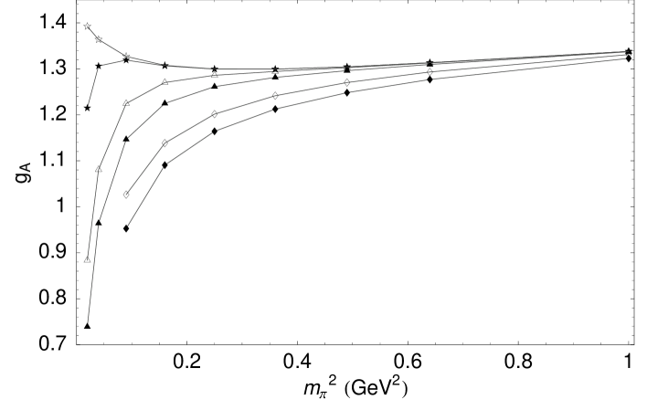
Figure 4: Plot of the axial coupling constant $g_{\scriptscriptstyle A}$ in the hedgehog versus $m_{\scriptscriptstyle\pi}^{2}$, as calculated on spherical volumes of radius $10$ fm (open star), $5$ fm (filled star), $3$ fm (open triangle), $2.5$ fm (filled triangle), $2$ fm (open diamond) and $1.8$ fm (filled diamond).

We see that the results for different volumes converge at large $m_{\scriptscriptstyle\pi}^{2}$, revealing very limited volume dependence in this region. This is what we expect to see because at large pion masses the pion field will die out quickly so that the effect of the boundary is minimal. At low $m_{\scriptscriptstyle\pi}$ the axial coupling constant exhibits large finite volume effects. Indeed, for the two lightest masses, $m_{\scriptscriptstyle\pi}=140$ MeV and $m_{\scriptscriptstyle\pi}=200$ MeV, the effect is very large, with $g_{\scriptscriptstyle A}$ decreasing by around $30\%$ and $50\%$ from $L=10$ to $2.5$ fm in each case. It is also interesting to note the turn-around in the low $m_{\scriptscriptstyle\pi}$ behaviour of $g_{\scriptscriptstyle A}$ between the $L=10$ fm and $L=5$ fm solutions.

4 Discussion

Our plot of the hedgehog axial coupling constant reveals a large volume dependence in the low $m_{\scriptscriptstyle\pi}$ region, with $g_{\scriptscriptstyle A}$ at the physical pion mass decreasing by over $50\%$ as the volume size decreases. This behaviour is similar to that observed in recent lattice QCD results. From the plots of the hedgehog solution in Fig. 3 we see that the important region to consider is the distance $L/2-R$ (where we once again use $L$ to denote the length of the side of the lattice). This is the distance between the edge of the baryon and the volume boundary. Inside the baryon bag the fields do not vary much with volume size. We expect that this conclusion is far more general than the particular model considered.

Clearly this has been a very simple study, involving a number of major approximations which must be remembered when considering our results. But by employing such a simple model we have been able to generate results over a wide range of volumes and pion masses with relative ease. Because of the exact nature of the solutions, at this point it would be very easy to examine the volume and mass dependence of other hedgehog properties. It would clearly be very interesting to employ a spontaneous symmetry breaking mechanism to include the pion and sigma masses.

4.1 Acknowledgments

This work was supported by the Australian Research Council and by the DOE under contract DE-AC05-84ER40150, under which SURA operates Jefferson Lab.

5 References

References

- [1] R. D. Young, D. B. Leinweber and A. W. Thomas, Prog. Part. Nucl. Phys. 50 (2003) 399 [arXiv:hep-lat/0212031].
- [2] D. B. Leinweber, A. W. Thomas and R. D. Young, Phys. Rev. Lett. 92 (2004) 242002 [arXiv:hep-lat/0302020].
- [3] M. Procura, T. R. Hemmert and W. Weise, Phys. Rev. D 69, 034505 (2004) [arXiv:hep-lat/0309020].
- [4] W. Detmold and M. J. Savage, Phys. Lett. B 599 (2004) 32 [arXiv:hep-lat/0407008].
- [5] S. R. Beane and M. J. Savage, Phys. Rev. D 70, 074029 (2004) [arXiv:hep-ph/0404131].
- [6] S. Sasaki, T. Blum, S. Ohta and K. Orginos [RBC Collaboration], Nucl. Phys. Proc. Suppl. 106 (2002) 302 [arXiv:hep-lat/0110053].
- [7] R. L. Jaffe, Phys. Lett. B 529 (2002) 105 [arXiv:hep-ph/0108015].
- [8] T. D. Cohen, Phys. Lett. B 529 (2002) 50 [arXiv:hep-lat/0112014].
- [9] A. Chodos and C. B. Thorn, Phys. Rev. D 12 (1975) 2733.
- [10] G. A. Miller, A. W. Thomas and S. Theberge, Phys. Lett. B 91 (1980) 192.
- [11] A. W. Thomas, Adv. Nucl. Phys. 13 (1984) 1.