IU-MSTP/65
                                                                                                               hep-lat/0501008
                                                                                                               January, 2005

Canonical Approach to Ginsparg-Wilson Fermion

Kosuke Matsui¹, Tomohiro Okamoto¹ and Takanori Fujiwara²

Abstract

Based upon the lattice Dirac operator satisfying the Ginsparg-Wilson relation, we investigate canonical formulation of massless fermion on the spatial lattice. For free fermion system exact chiral symmetry can be implemented without species doubling. In the presence of gauge couplings the chiral symmetry is violated. We show that the divergence of the axial vector current is related to the chiral anomaly in the classical continuum limit. PACS: 11.15.-q, 11.15.Ha, 12.38.Gc

1 Introduction

The discovery of lattice Dirac operators satisfying the Ginsparg-Wilson (GW) relation [1, 2, 3] enables us to implement exact chiral symmetry on the lattice [4, 5] without suffering from species doubling [6]. The overlap Dirac operator [3], for instance, not only possesses all the desired classical properties such as the continuum limit and locality [7] but also reproduces correct chiral anomaly [8, 9]. The lattice Dirac action with the exact chiral symmetry may be considered as a correct starting point of the nonperturbative studies of gauge theories with massless fermions [10, 11].

In lattice gauge theories it is usual to employ euclidean path integral formalism. The main concern there is to compute various physical quantities nonpertubatively. To investigate formal aspects of the theory concerning states and operators it is suitable to work in canonical approach. To the author’s knowledge, canonical treatment of GW fermion has only been investigated by Creutz, Horváth and Neuberger [12]. They found an interesting characteristic structure of the spectra of energy and axial charge leading to axial anomaly. In this paper we will pursue the validity of their approach further and establish the chiral anomaly in the classical continuum limit.

On the full eucliean lattice, it is possible to give action with exact chiral invariance at the classical level [5]. The fermion measure, however, is not chiral invariant but gives raise to nontrivial Jacobian [13, 5]. It reproduces chiral anomaly in the classical continuum limit [8, 9]. In the canonical approach time is a continuous coordinate and only the spatial coordinates are discretized. This causes a problem in constructing chirally symmetric action.

To put this more precisely, we consider a Dirac operator

$$D=i\gamma^{0}{\cal D}_{0}+D_{d-1}~{},$$ (1.1)

where ${\cal D}_{0}$ is the time component of the ordinary covariant derivative in the continuum and $D_{d-1}$ is the spatial part of $D$. It is assumed to satisfy the GW relation. If we choose $D_{d-1}$ to be the overlap operator, species doublers can be avoided. The full Dirac operator $D$, however, does not satisfy the GW relation even in the absence of gauge couplings. Nevertheless it is possible to define exact chiral symmetry in the free field case. The chiral transformation there is analogous to the one given in Ref. [5]. The axial charge of a free GW fermion depends on momentum. In the physical momentum region it is almost constant as in the continuum theory. The separation of positive and negative axial charges decreases as the energy increases. It vanishes at the doubler momenta. In other words the states with positive axial charge and those with negative one are smoothly connected with one another at the boundaries of the first Brillouin zone [12].

In the presence of gauge couplings, the chiral transformation becomes field dependent. It is no more a symmetry of the action. This is quite different with the conventional euclidean approach. The violation of the chiral symmetry is not a bad news. We expect it from the beginning since the chiral symmetry must be broken in any regulalized theory, otherwise we could not reproduce the chiral anomaly. We show that certain gauge fields induce asymmetric flow in the spectrum that leads to nonconservation of the axial charge. This is the origin of chiral anomaly.

The interpretation of axial anomaly that external gauge fields can generate asymmetric level shifts of the negative energy states in the Dirac sea is well-known in the continuum theory [14]. Similar analysis has been be carried out also for Wilson fermion. In this case the chiral symmetry, however, is broken break by the Wilson term even in the absence of gauge couplings. The axial anomaly for Wilson fermions was obtained in Ref. [18] and its physical picture was investigated in Ref. [15].

This paper is organized as follows. In the next section we consider free GW fermion and introduce exact chiral symmetry. In Sect. 3 we examine the effects of couplings with the gauge fields on the chiral symmetry and give the axial current divergence. In Sect. 4 we describe the canonical approach explicitly for a two-dimensional system and examine the conservation of the axial charge for an adiabatically changing external electric field. In Sect. 5 we compute the classical continuum limit of the axial current divergence in an arbitrary smooth background and show that the chiral anomaly is correctly reproduced. Sect. 6 is devoted to summary and discussion. We collect notation in Appendix A. The technical detail in carrying out the momentum integrations to compute the anomaly coefficients is given in Appendix B.

2 Exact Chiral Symmetry

In this section we consider canonical formulation of a lattice Dirac theory in an arbitrary even dimensional space-time with continuous time $t$ and $d-1$ discretized lattice coordinates $x$. The signature is assumed to be minkowskian and the spatial part is hypercubic regular lattice with lattice spacing $a$. The massless fermion action can be generically written as

$$S_{F} = a^{d-1}\sum_{x}\int dt\overline{\psi}\Biggl{(}i\gamma^{0}\frac{\partial}{\partial t}+D_{d-1}\Biggr{)}\psi~{},$$ (2.1)

where $D_{d-1}$ stands for the spatial part of the lattice Dirac operator. Unlike euclidean formulation $\psi$ and $\overline{\psi}$ are related by the Dirac conjugate

$$\overline{\psi}=\psi^{\dagger}\gamma^{0}~{}.$$ (2.2)

The conventions for the metric and $\gamma$-matrices are summarized in Appendix A.

To keep the fermion massless while avoiding species doubling, we employ the following construction analogous to the overlap operator

$$D_{d-1}=\frac{1}{a}\Biggl{(}1+\gamma_{d+1}\frac{H_{d-1}}{\sqrt{H_{d-1}^{2}}}\Biggr{)}~{},$$ (2.3)

where $H_{d-1}$ is the hermitian Wilson-Dirac operator given by

$$H_{d-1}=\gamma_{d+1}(aD_{W}^{(d-1)}-m)~{},\qquad D_{W}^{(d-1)}=\sum_{k=1}^{d-1}(i\gamma^{k}\partial_{k}^{S}-r\partial_{k}^{A})~{}.$$ (2.4)

The $\partial_{k}^{S}$ and $\partial_{k}^{A}$ are, respectively, symmetric and antisymmetric difference operators defined by (A.4) and $D_{W}^{(d-1)}$ is nothing but the Wilson-Dirac operator with the difference along the $d$-th (euclidean time) axis omitted. This choice is consistent with the cubic symmetry of the underlying lattice. The $r$ and $m$ are parameters. They must be so chosen that the theory contains no doublers. Here we assume $r>0$.

The Dirac operator (2.3) satisfies the following relations

$$\gamma_{d+1}D_{d-1}+D_{d-1}\gamma_{d+1}=aD_{d-1}\gamma_{d+1}D_{d-1}~{},\qquad\gamma^{0}D_{d-1}+D_{d-1}\gamma^{0}=aD_{d-1}\gamma^{0}D_{d-1}~{},$$ (2.5)

where the first is the Ginsparg-Wilson relations as in the case of overlap Dirac operator on full euclidean lattices. The second one is specific to the present canonical approach. It can be seen by noting the fact that $D_{d-1}$ commutes with $\gamma^{0}\gamma_{d+1}=i^{\frac{d}{2}-1}\gamma^{1}\dots\gamma^{d-1}$. It also satisfies the following hermiticity

$$D_{d-1}^{\dagger}\gamma^{0}=\gamma^{0}D_{d-1}~{},\quad D_{d-1}^{\dagger}\gamma_{d+1}=\gamma_{d+1}D_{d-1}~{}.$$ (2.6)

From the action (2.1) we define single-particle hamiltonian $h$ by

$$h=-\gamma^{0}D_{d-1}~{}.$$ (2.7)

The hermiticity of $h$ can be seen from the $\gamma^{0}$ hermiticity (2.6).

In the absence of the interaction with gauge field the action (2.1) is invariant under the lattice chiral transformation

$$\delta\psi=i\epsilon\gamma_{d+1}\Biggl{(}1-\frac{a}{2}D_{d-1}\Biggr{)}\psi~{},\qquad\delta\overline{\psi}=i\epsilon\overline{\psi}\Biggl{(}1-\frac{a}{2}D_{d-1}\Biggr{)}\gamma_{d+1}~{},$$ (2.8)

where $\epsilon$ is an arbitrary real parameter. These chiral transformations are consistent with the Dirac conjugate (2.2) and the hermiticity of $D_{d-1}$.

The invariance of the action under the chiral symmetry also implies that the axial charge operator $q_{d+1}$ defined by

$$q_{d+1}=\gamma_{d+1}\Biggl{(}1-\frac{a}{2}D_{d-1}\Biggr{)}~{}.$$ (2.9)

commutes with $h$. Furthermore, $h$ and $q_{d+1}$ satisfy [12]

$$\frac{a^{2}}{4}h^{2}+q_{d+1}^{2}=1~{}.$$ (2.10)

These can be checked directly by using (2.5) and (2.6). We thus see that $(aE/2,Q_{d+1})$ with $E$ and $Q_{d+1}$, respectively, the eigenvalues of $h$ and $q_{d+1}$ can be regarded as a point on the unit circle and unlike the continuum theory the axial charge depends on the energy of the state.

To see the doubling problem we go over to momentum representation

$$\psi(t,x)=u(p)e^{i(px-Et)}~{}.\qquad\Bigl{(}px=\sum_{k=1}^{d-1}p^{k}x^{k}\Bigr{)}$$ (2.11)

To parametrize the eigenvalues of $h$ and $q_{d+1}$ it is convenient to introduce $d$-dimensional orthonormal coordinates $n$ by

$$n^{k}=\rho\sin ap^{k}~{},\qquad n_{d}=-\rho\Bigl{(}r\sum_{k=1}^{d-1}(\cos ap^{k}-1)+m\Bigr{)}~{},$$

$$\rho^{-1}=\sqrt{\sum_{k=1}^{d-1}\sin^{2}ap^{k}+\Biggl{(}r\sum_{k=1}^{d-1}(\cos ap^{k}-1)+m\Biggr{)}^{2}}~{}.$$ (2.12)

These define a mapping from $T^{d-1}$, the 1st Brillouin zone $-\frac{\pi}{a}<p^{k}\leq\frac{\pi}{a}$ with the opposite boundaries identified, to $S^{d-1}$. The energy eigenvalues $E$ and the axial charge $Q_{d+1}$ are given by

$$\frac{a}{2}E=\pm\sqrt{\frac{1+n_{d}}{2}}~{},\qquad Q_{d+1}=\pm\sqrt{\frac{1-n_{d}}{2}}~{}.$$ (2.13)

Doublers appear at $p^{k}=0$ or $\pi/a$ except for the origin $p^{k}=0$ if $n_{d}=-1$ is simultaneously satisfied. For $0<m/r<2$ the energy $E$ vanishes only at the origin .

In quantum theory we impose the equal-time anticommutation relations

$$\{\psi_{\alpha}(t,x),\psi^{\dagger}_{\beta}(t,y)\}=\delta_{\alpha\beta}\delta_{x,y}/a^{d-1}~{},\quad\{\psi_{\alpha}(t,x),\psi_{\beta}(t,y)\}=\{\psi^{\dagger}_{\alpha}(t,x),\psi^{\dagger}_{\beta}(t,y)\}=0~{},$$ (2.14)

where $\alpha$ and $\beta$ are spinor indices. The hamiltonian, the fermion number and the axial charge are given by

$${\cal H} = a^{d-1}\sum_{x}\psi^{\dagger}h\psi~{},$$ (2.15)

$${\cal Q} = a^{d-1}\sum_{x}\psi^{\dagger}\psi~{},$$ (2.16)

$${\cal Q}_{d+1} = a^{d-1}\sum_{x}\psi^{\dagger}q_{d+1}\psi~{}.$$ (2.17)

By expanding the field operators in terms of plane wave solutions with definite energy and axial charge, we can introduce creation and annihilation operators. In Sect. 4 we will explicitly carry out this in $(1+1)$-dimensions.

3 Coupling with Gauge Fields

We now introduce the coupling with gauge field. This can be achieved by simply replacing the time-derivative with the covariant derivative ${\cal D}_{0}=\partial/\partial t+A_{0}$ and the differences $\partial_{k}$, $\partial_{k}^{\ast}$ with the covariantized operators $\nabla_{k}$ and $\nabla_{k}^{\ast}$ defined by (A). The fermion action (2.1) is then replaced by

$$S_{F} = a^{d-1}\sum_{x}\int dt~{}\overline{\psi}(i\gamma_{0}{\cal D}_{0}+D_{d-1})\psi~{}.$$ (3.1)

This is invariant under the gauge transformation

$$\psi(t,x) \rightarrow \Lambda(t,x)\psi(t,x)$$

$$A_{0}(t,x) \rightarrow \Lambda(t,x)A_{0}(t,x)\Lambda^{\dagger}(t,x)-\partial_{t}\Lambda(t,x)\Lambda^{\dagger}(t,x)$$ (3.2)

$$U_{k}(t,x) \rightarrow \Lambda(t,x)U_{k}(t,x)\Lambda^{\dagger}(t,x+a\hat{k})~{},$$

where $\hat{k}$ is the unit vector in the $k$-the direction and $U_{k}(t,x)$ is the link variable associated with the link $(x,x+a\hat{k})$.

If we consider the gauge fields as dynamical, we must also introduce their kinetic part to the action. The magnetic part of the field strengths can be defined from the standard plaquette variables

$$P_{kl}(t,x)=U_{k}(t,x)U_{l}(t,x+a\hat{k})U_{k}^{\dagger}(t,x+a\hat{l})U_{l}^{\dagger}(t,x)~{}.$$ (3.3)

The electric field is given by

$$E_{k}(t,x)=-\nabla_{k}A_{0}(t,x)+\frac{1}{a}\dot{U}_{k}(t,x)U_{k}^{\dagger}(t,x)~{}.$$ (3.4)

The Wilson action for the gauge field takes the form

$$S_{G}=-a^{d-1}\sum_{x}\int dt\frac{1}{g^{2}}{\rm tr}(E_{k})^{2}-a^{d-1}\sum_{x}\int dt\sum_{k<l}\frac{1}{a^{4}g^{2}}{\rm tr}(2-P_{kl}-P_{kl}^{\dagger})~{},$$ (3.5)

where $g$ is the coupling constant.

In general the overlap Dirac operator becomes singular for gauge fields where the hermitian Wilson-Dirac operator has a zero-mode. This implies that the fermion action (3.1) is not a well-defined functional over the entire space of the link variables. It is well-known in the euclidean path integral formulation that the overlap Dirac operator is well-defined for gauge field satisfying so-called admissibility condition

$$||1-P_{kl}||<\varepsilon~{},$$ (3.6)

where $||\cdots||$ stands for operator norm and $\varepsilon$ is some positive constant depending on the parameters $r$, $m$ and the dimensionality $d$ [7]. By excising nonadmissible configurations the space of lattice gauge fields acquires nontrivial topological structure. The admissibility condition helps to define the chiral and gauge anomalies precisely in the full euclidean lattice theory.

Practically, nonadmissible gauge fields can be avoided by modifying the gauge field action so that they are decoupled from the system [10]. Incidentally, in $(1+1)$ dimensions there is a parameter region of $r$ and $m$ where the overlap Dirac operator $D_{1}$ can be defined for any gauge field. This case is of great interest since the system corresponds to the lattice regularization of the massless Schwinger model. In the remainder of this paper we shall consider the lattice gauge fields as background external field.

The chiral transformation (2.8), however, is not consistent with the coupling of the gauge field. The spatial part of the fermion action (3.1) is invariant by construction. However, the term containing time-derivative violates the symmetry. The difficulty comes from the noncommutativity of ${\cal D}_{0}$ and $D_{d-1}$. In fact under the variation (2.8) with $\epsilon$ being an arbitrary local parameter the action changes as

$$\delta S_{F} = ia^{d-1}\sum_{x}\int dt~{}\overline{\psi}\Biggl{(}i\gamma_{0}\gamma_{d+1}\dot{\epsilon}\Bigl{(}1-\frac{a}{2}D_{d-1}\Bigr{)}-\frac{ia}{2}\gamma_{0}\gamma_{d+1}\epsilon[{\cal D}_{0},D_{d-1}]$$ (3.7)

$$\hskip 85.35826pt+[\epsilon,D_{d-1}]\gamma_{d+1}\Bigl{(}-1+\frac{a}{2}D_{d-1}+\frac{a}{2}(i\gamma_{0}{\cal D}_{0}+D_{d-1})\Bigr{)}\Biggr{)}\psi~{}.$$

If $\epsilon$ is a constant parameter, the first and the last term in the integrand are absent. Hence the chiral symmetry is violated if $[{\cal D}_{0},D_{d-1}]$ is nonvanishing. Incidentally, we can retain the chiral invariance for static gauge fields in the temporal gauge $A_{0}=0$.

The variation (3.7) of the action leads to the axial current divergence relation

$$\frac{\partial}{\partial t}\Bigl{\{}\overline{\psi}\gamma_{0}\gamma_{d+1}\Bigl{(}1-\frac{a}{2}\overrightarrow{D}_{d-1}\Bigr{)}\psi\Bigr{\}}-i\overline{\psi}(\overrightarrow{D}_{d-1}-\overleftarrow{D}_{d-1})\gamma_{d+1}\Bigl{(}1-\frac{a}{2}\overrightarrow{D}_{d-1}\Bigr{)}\psi=-\frac{a}{2}\overline{\psi}\gamma_{0}\gamma_{d+1}[{\cal D}_{0},\overrightarrow{D}_{d-1}]\psi~{},$$

where we have introduced the following notation to simplify the expressions

$$\overrightarrow{D}_{d-1}\psi=D_{d-1}\psi(t,x)~{},\qquad\overline{\psi}\overleftarrow{D}_{d-1}=\overline{\psi}D_{d-1}(t,x)~{}.$$ (3.9)

The axial charge density appearing in the time derivative of this expression coincides with (2.17). The second term on the lhs of (3) corresponds to spatial divergence of the axial current. In fact the integral of this term over the spatial lattice vanishes. This can be seen by noting the relation like

$$a^{d-1}\sum_{x}\overline{\psi}\overleftarrow{D}_{d-1}\psi=a^{d-1}\sum_{x}\overline{\psi}\overrightarrow{D}_{d-1}\psi=a^{d-1}\sum_{x}\overline{\psi}D_{d-1}\psi~{}.$$

What we have seen is that in the presence of the couplings with an external gauge fields the commutativity of $D_{d-1}$ with the time derivative is lost and consequently the chiral symmetry (2.8) is violated. In Sect. 5 we will show that the violation of the chiral symmetry, the rhs of (3), which is naively of ${\rm O}(a)$, reproduces the chiral anomaly in the classical continuum limit.

Since the chiral transformation (2.8) is not an exact symmetry, we may consider naive chiral transformations

$$\delta\psi=i\epsilon\gamma_{d+1}\psi~{},\qquad\delta\overline{\psi}=i\epsilon\overline{\psi}\gamma_{d+1},$$ (3.10)

which is not a symmetry of the action as well. We close this section with a comment on what happens if one uses naive chiral transformations instead of (2.8) in the evaluation of chiral anomaly. The variation of the action (3.1) under the naive chiral transformation gives the following axial current divergence

$$\frac{\partial}{\partial t}\{\overline{\psi}\gamma^{0}\delta_{d+1}\psi\}-i\overline{\psi}(\overrightarrow{D}_{d-1}-\overleftarrow{D}_{d-1})\psi=-ia\overline{\psi}\overrightarrow{D}_{d-1}\gamma_{d+1}D_{d-1}\psi.$$ (3.11)

Compared with (3), we arrive at an apparently different form of chiral anomaly if we employ (3.10) as the chiral transformation. These two, however, differ only by a total divergence of some gauge invarinat current $k^{\mu}$ as can be seen from

$$-ia\overline{\psi}\overrightarrow{D}_{d-1}\gamma_{d+1}D_{d-1}\psi=-\frac{a}{2}\overline{\psi}\gamma_{0}\gamma_{d+1}[{\cal D}_{0},\overrightarrow{D}_{d-1}]\psi+\dot{k}^{0}+\partial_{l}^{\ast}k^{l}$$ (3.12)

where $k^{\mu}$ is defined by the relations

$$k^{0}=\frac{a}{2}\overline{\psi}\gamma_{0}\gamma_{d+1}\overrightarrow{D}_{d-1}\psi,\qquad\partial_{l}^{\ast}k^{l}=-\frac{ia}{2}\overline{\psi}(\overrightarrow{D}_{d-1}-\overleftarrow{D}_{d-1})\gamma_{d+1}\overrightarrow{D}_{d-1}\psi\quad(l=1,2,3).$$ (3.13)

The axial currents corresponding to the transformations (2.8) and (3.10) differ only by a gauge invariant current of O$(a)$ and give essentially the same chiral anomaly in the classical continuum limit.

4 Ginsparg-Wilson Fermion in $(1+1)$-dimensions

In this section we apply the formalism developed in the preceding sections to the case of $(1+1)$-dimensions. We consider a finite periodic lattice of size $L=a(2N+1)$, where we have assumed that the number of sites is odd. This is only a technical assumption to make the arguments simple.

In momentum space the eigenspinors satisfy the Dirac equation

$$\gamma^{0}Eu(p)+D_{1}(p)u(p)=0~{},\qquad D_{1}(p)=\frac{1}{a}(\gamma^{1}n_{1}+n_{2}+1)~{},$$ (4.1)

where $D_{1}(p)$ is the overlap operator in momentum space. In $(1+1)$-dimensions the eigenspinors can be more conveniently parametrized by a pseudo-momentum $\tilde{p}$ defined by

$$\sin a\tilde{p}=-n_{1}=\frac{\sin ap}{\sqrt{\sin^{2}ap+(r(\cos ap-1)+m)^{2}}}~{},$$

$$\cos a\tilde{p}=-n_{2}=\frac{r(\cos ap-1)+m}{\sqrt{\sin^{2}ap+(r(\cos ap-1)+m)^{2}}}~{}.$$ (4.2)

For $0<m/r<2$ these define one-to-one mapping from $-\pi/a<p\leq\pi/a$ to $-\pi/a<\tilde{p}\leq\pi/a$. We consider $\tilde{p}$ as continuous function of $p$ beyond the first Brillouin zone. In particular we have

$$\widetilde{p+\frac{2\pi}{a}}=\tilde{p}+\frac{2\pi}{a}~{}.$$ (4.3)

One easily see from (2) that the choice $r=m=1$ leads to $\tilde{p}=p$. In $(1+1)$-dimensions this parameter choice is special in the sense that the overlap operator $D_{1}$ becomes identically equal to the Wilson operator. This can be verified directly by establishing the relation $H_{1}^{2}=1$. Remarkably, it holds true even in the presence of gauge couplings.

The eigenspinor for $E\neq 0$ is automatically eigenspinor for the chiral operator $q_{3}$ defined by (2.9). We thus find plane wave solutions for $\displaystyle{E=E_{p}=\frac{2}{a}\sin{\frac{a\tilde{p}}{2}}}$ and $\displaystyle{Q_{3}=\chi_{p}=\cos\frac{a\tilde{p}}{2}}$

$$U_{Rp}(t,x)=\frac{1}{\sqrt{L}}u_{R}(p)e^{i(px-E_{p}t)}~{},\qquad u_{R}(p)=\left(\begin{matrix}\displaystyle{\cos\frac{a\tilde{p}}{4}}\\ \displaystyle{-\sin\frac{a\tilde{p}}{4}}\end{matrix}\right)$$ (4.4)

and for $\displaystyle{E=-E_{p}=-\frac{2}{a}\sin{\frac{a\tilde{p}}{2}}}$ and $\displaystyle{Q_{3}=-\chi_{p}=-\cos\frac{a\tilde{p}}{2}}$

$$U_{Lp}(t,x)=\frac{1}{\sqrt{L}}u_{L}(p)e^{i(px+E_{p}t)}~{},\qquad u_{L}(p)=\left(\begin{matrix}\displaystyle{\sin\frac{a\tilde{p}}{4}}\\ \displaystyle{\cos\frac{a\tilde{p}}{4}}\end{matrix}\right)~{}.$$ (4.5)

The dispersion relations $E=\pm E_{p}$ are easily recognized as the lattice analog of $E=\pm p$ known for the continuum chiral theory. Unlike the fermion number the conserved axial charge depends on the momentum. For the physical region $|p|<\hskip-2.84544pt<\pi/a$ the axial charge is $Q_{3}=\pm\chi_{p}\approx\pm 1$. It approaches to zero at the boundaries of the 1st Brillouin zone $|p|\approx\pi/a$.

The momentum $p$ is usually restricted to lie in the 1st Brillouin zone. In the present chiral theory the period of the spectra of energy and axial charge is not $2\pi/a$ but is $4\pi/a$. Furthermore, the wave functions (4.4) and (4.5) up to an overall sign are transformed into each other by the translation $p\rightarrow p+2\pi/a$. As will be clear shortly, it turns out to be convenient to double the Brillouin zone and use a single wave function defined by

$$U_{p}(t,x)=\frac{1}{\sqrt{L}}u(p)e^{i(px-E_{p}t)}~{},\qquad u(p)=\left(\begin{matrix}\displaystyle{\cos\frac{a\tilde{p}}{4}}\\ \displaystyle{-\sin\frac{a\tilde{p}}{4}}\end{matrix}\right)~{}.$$ (4.6)

By noting the relation (4.3) we see that up to an overall sign $U_{p}$ is periodic in $p$ with a period $4\pi/a$ and $U_{p}=U_{Rp}$ for $-\pi<ap<\pi$ and $U_{p}=U_{Lp-2\pi/a}$ for $\pi<ap\leq 3\pi$. The relation among the momentum, the energy and the axial charge are shown in Fig. 1.

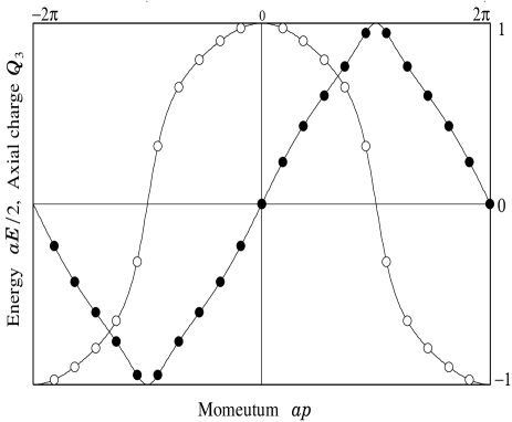
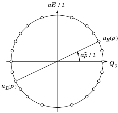
Figure 1: The energy ($\bullet$) and the axial charge ($\circ$) are plotted as functions of momentum for $r=0.8$ and $m=1.2$ with $N=5$ (left). They are conveniently described as points on a unit circle (right) [12]. Diametrically opposite points correspond to a pair of eigenspinor $u_{R}(p)$ and $u_{L}(p)$.

The free Dirac field can be expanded in terms of $U_{p}$ as

$$\psi(t,x)=\sum_{0\leq ap<4\pi}a_{p}U_{p}(t,x)~{},$$ (4.7)

where $a_{p}$ is a creation or an annihilation operators satisfying the anti-commutation relations

$$\{a_{p},a^{\dagger}_{p^{\prime}}\}=\delta_{p,p^{\prime}}~{},\quad\{a_{p},a_{p^{\prime}}\}=\{a^{\dagger}_{p},a^{\dagger}_{p^{\prime}}\}=0~{}.\qquad(0\leq p,~{}p^{\prime}<4\pi/a)$$ (4.8)

We see from (4.6) that $a_{p}^{\dagger}$ creates a particle of energy $E_{p}$ for $0\leq p\leq 2\pi/a$ and $a_{p}$ create an anti-particles of energy $|E_{p}|=-E_{p}$ for $2\pi/a<p<4\pi/a$, where we have assigned the zero-energy states as particles for simplicity.

The hamiltonian $H$, the fermion number ${\cal Q}$ and the axial charge ${\cal Q}_{3}$ are given by

$$H=a\sum_{x}\psi^{\dagger}h\psi=\sum_{0\leq ap<4\pi}E_{p}a_{p}^{\dagger}a_{p}~{},$$ (4.9)

$${\cal Q}=a\sum_{x}\psi^{\dagger}\psi=\sum_{0\leq ap<4\pi}a_{p}^{\dagger}a_{p}~{},$$ (4.10)

$${\cal Q}_{3}=a\sum_{x}\psi^{\dagger}q_{3}\psi=\sum_{0\leq ap<4\pi}\chi_{p}a_{p}^{\dagger}a_{p}~{}.$$ (4.11)

These are not normal ordered with respect to the creation and annihilation operators and the energy and the fermion number of the Dirac vacuum are nonvanishing. However, the axial charge of the Dirac vacuum vanishes because of the cancellation of the axial charge between the occupied negative energy states.

We now introduce $U(1)$ lattice gauge field $(A_{0}(t,x),U_{1}(t,x))$ in $(1+1)$-dimensions and investigate the behavior of the axial charge. In the remainder of this section we assume that the gauge potential is real. The electric field defined by (3.4) is given by

$${\cal E}(t,x)=-\partial_{1}A_{0}(t,x)-\frac{i}{a}\partial_{t}U_{1}(t,x)U_{1}(t,x)^{\dagger}~{},$$ (4.12)

which is invariant under the gauge transformation (3). In this section we are only interested in a spatially uniform electric field generated by the gauge field

$$A_{0}(t,x)=0~{},\qquad U_{1}(t,x)=e^{-iaA(t)}~{}.$$ (4.13)

Then the electric field is given by

$${\cal E}(t)=-\dot{A}(t)~{}.$$

Since the gauge field is translation invariant in the spatial direction, we can solve the Dirac equation in momentum space. In the presence of the background gauge field the free hamiltonian $-\gamma^{0}D_{1}(p)$ is modified to $-\gamma^{0}D_{1}(p-A(t))$. Then the Dirac equation in momentum space is simply given by

$$i\frac{\partial\varphi(t,p)}{\partial t} = -\gamma^{0}D_{1}(p-A(t))\varphi(t,p)~{},$$ (4.14)

At this point, we further assume that the $A(t)$ changes adiabatically from $A(t_{i})=0$ to

$$A(t_{f})=q=\frac{2\pi n_{q}}{a(2N+1)}~{},$$ (4.15)

where $n_{q}$ is an integer satisfying $|n_{q}|\leq N$. We take $t_{f}-t_{i}$ sufficiently large so that the adiabatic change of $A(t)$ is possible. In this situation the transitions between $u_{R}$ and $u_{L}$ are suppressed and a state that is initially in an eigenstate of the hamiltonian keeps staying in the corresponding eigenstate of the hamiltonian at an arbitrary time. Thus the solution to the Dirac equation (4.14) satisfying $\varphi(t_{i},p)=u(p)$ can be solved in terms of the eigenspinor of $-\gamma^{0}D_{1}(p-A(t))$ as

$$\varphi(t,p)=u(p-A(t))\exp\Biggl{[}-i\int_{t_{i}}^{t}E_{p-A(\tau)}d\tau\Biggr{]}~{},$$ (4.16)

where $u(p)$ is given by (4.6) and $E_{p}=\displaystyle{\frac{2}{a}\sin\frac{a\tilde{p}}{2}}$. Under the influence of the background electric field the free Dirac field (4.7) evolves to

$$\psi(t,x)=\frac{1}{\sqrt{L}}\sum_{0\leq ap<4\pi}a_{p}u(p-A(t))\exp\Biggl{[}i\Biggl{(}px-\int_{t_{i}}^{t}E_{p-A(\tau)}d\tau+\delta_{p}\Biggr{)}\Biggr{]}~{}.$$ (4.17)

The phase $\delta_{p}$ is chosen so that $\psi(t,x)$ reduces to the free field (4.7) for $t\leq t_{i}$.

For $t\geq t_{f}$ the Dirac field approaches to

$$\psi(t,x)=\frac{1}{\sqrt{L}}e^{iqx}\sum_{0\leq ap<4\pi}a_{p}u(p-q)e^{i((p-q)x-E_{p-q}t+\delta^{\prime}_{p})}~{},$$ (4.18)

where $\delta^{\prime}_{p}$ is some irrelevant phase.

The overall factor $e^{iqx}$ is periodic on the lattice if the condition (4.15) is satisfied. It can be removed by carrying out a time-independent gauge transformation

$$\psi(t,x)\rightarrow e^{-iqx}\psi(t,x)~{}.$$ (4.19)

This transforms $\psi(t,x)$ $(t>t_{f})$ into a free field. As an external gauge field, it is not necessary to impose the condition (4.15) and any $q=A(t_{f})$ is allowed. In general $e^{iqx}$, however, is not periodic on the lattice and cannot be regarded as a gauge transformaiton on the lattice. Only those satisfying (4.15) can be eliminated by the gauge transformaiton (4.19).

What we found is that the state with initial momentum $p$ is carried over to the state with momentum $p-q$ due to the electric field exerted on the system. It is well-known in continuum theory that this kind of spectral flow results in the violation of the conservation of the axial charge. To see this we compute the vacuum expectation value of the axial charge at $t=t_{f}$. It is given by

$$\langle 0|{\cal Q}_{3}(t_{f})|0\rangle = \sum_{0\leq ap<4\pi}\cos\frac{a\widetilde{(p-q)}}{2}\langle 0|a^{\dagger}_{p}a_{p}|0\rangle$$ (4.20)

$$= \sum_{0<ap<\pi}\Biggl{(}\cos\frac{a\widetilde{(p+q)}}{2}-\cos\frac{a\widetilde{(p-q)}}{2}\Biggr{)}$$

$$= \sum_{\pi-2aq<ap<\pi}\cos\frac{a\widetilde{(p+q)}}{2}-\sum_{0<ap\leq 2aq}\cos\frac{a\widetilde{(p-q)}}{2}~{}.$$

where $|0\rangle$ is the Dirac vacuum satisfying $a_{p}|0\rangle=0$ for $0\leq ap\leq 2\pi$ and use has been made of (4.3). In the last equality we have assumed $q>0$. The contributions from the modes lying near the boundary of the Brillouin zone ($\pi-2aq<ap<\pi$) are canceled out and only the modes around the origin ($0<ap\leq 2aq$) contribute to the violation of the axial charge conservation. We thus find

$$\langle 0|{\cal Q}_{3}(t_{f})|0\rangle = -\sum_{-aq<ap\leq aq}\cos\frac{a\widetilde{p}}{2}~{}.$$ (4.21)

The $q<0$ case can be analyzed in a similar way.

To relate (4.21) with the axial anomaly we consider the classical continuum limit $a\rightarrow 0$ with $L=a(2N+1)$ kept fixed. For the modes contributing to the nonvanishing axial charge we have $\displaystyle{\cos\frac{a\tilde{p}}{2}\rightarrow 1}$ as $a\rightarrow 0$. We thus find

$$\langle 0|{\cal Q}_{3}(t_{f})|0\rangle\mathop{=}_{a\rightarrow 0}-2n_{q}=-\frac{1}{\pi}a(2N+1)q=\frac{1}{\pi}a\sum_{x}\int_{t_{i}}^{t_{f}}{\cal E}(t)dt~{},$$

where use has been made of ${\cal E}(t)=-\dot{A}(t)$. Since $\langle 0|{\cal Q}_{3}(t_{i})|0\rangle=0$, we finally obtain

$$\int_{t_{i}}^{t_{f}}dt\langle 0|\dot{\cal Q}_{3}(t)|0\rangle\mathop{=}_{a\rightarrow 0}2\frac{1}{2\pi}\int_{0}^{L}dx\int_{t_{i}}^{t_{f}}dt{\cal E}(t)~{}.$$ (4.22)

This coincides with the integrated axial anomaly relation.

The nonconservation of the axial charge implies the violation of the chiral symmetry. In the next section we investigate the chiral symmetry in the presence of an arbitrary background gauge field and see how the chiral anomaly is reproduced in the classical continuum limit.

5 Chiral Anomaly

In the presence of a background gauge field the chiral symmetry is violated. We will compute the violation of the axial charge by examining the classical continuum limit of the vacuum expectation value of the operator appearing in the rhs of (3). It is a local function of the gauge field and is denoted by $2{\cal A}(t,x)$

$${\cal A}(t,x) = -\frac{a}{4}\langle\overline{\psi}(t,x)\gamma_{0}\gamma_{d+1}[{\cal D}_{0},D_{d-1}]\psi(t,x)\rangle$$

$$= -\frac{a}{4}\lim_{t^{\prime}\rightarrow t}\lim_{x^{\prime}\rightarrow x}{\rm tr}\gamma_{d+1}\gamma^{0}[{\cal D}_{0},D_{d-1}]\langle{\rm T}\psi(t,x)\overline{\psi}(t^{\prime},x^{\prime})\rangle~{},$$

where ${\rm tr}$ stands for trace over spin and internal indices and ${\rm T}$ denotes time-ordering. The two-point function $\langle{\rm T}\psi(t,x)\overline{\psi}(t^{\prime},x^{\prime})\rangle$ satisfies

$$(i\gamma^{0}{\cal D}_{0}+D_{d-1})\langle{\rm T}\psi(t,x)\overline{\psi}(t^{\prime},x^{\prime})\rangle=i\delta(t-t^{\prime})\delta_{x,x^{\prime}}/a^{d-1}~{}.$$ (5.1)

Hence ${\cal A}$ can be written as

$${\cal A}(t,x) = -\frac{i}{4a^{d-2}}\lim_{t^{\prime}\rightarrow t}\lim_{x^{\prime}\rightarrow x}{\rm tr}\gamma_{d+1}\gamma^{0}[{\cal D}_{0},D_{d-1}]\frac{1}{i\gamma^{0}{\cal D}_{0}+D_{d-1}+i\epsilon}\delta(t-t^{\prime})\delta_{x,x^{\prime}}~{},$$ (5.2)

where the $i\epsilon$ prescription is made explicit. For simplicity we assume that the size of the lattice is infinite. The rhs of this expression can be simplified by making use of the relation

$$\delta(t-t^{\prime})\delta_{x,x^{\prime}}=\int_{-\infty}^{+\infty}\frac{dE}{2\pi}e^{-iE(t-t^{\prime})}\int_{-\pi}^{\pi}\frac{d^{d-1}p}{(2\pi)^{d-1}}e^{ip(x-x^{\prime})/a}~{}.$$ (5.3)

After a bit of algebra, we find

$${\cal A}(t,x) = -\frac{i}{4a^{d-2}}\int_{-\infty}^{+\infty}\frac{dE}{2\pi}\int_{-\pi}^{\pi}\frac{d^{d-1}p}{(2\pi)^{d-1}}{\rm tr}\;\gamma_{d+1}\gamma^{0}[{\cal D}_{0},\tilde{D}_{d-1}]\frac{1}{i\gamma^{0}{\cal D}_{0}+\gamma^{0}E+\tilde{D}_{d-1}+i\epsilon}$$ (5.4)

$$= -\frac{i}{4a^{d-1}}\int_{-\infty}^{+\infty}\frac{dE}{2\pi}\int_{-\pi}^{\pi}\frac{d^{d-1}p}{(2\pi)^{d-1}}{\rm tr}\;\gamma_{d+1}\gamma^{0}\Biggl{[}{\cal D}_{0},\gamma_{d+1}\frac{\tilde{H}_{d-1}}{\sqrt{\tilde{H}_{d-1}^{2}}}\Biggr{]}$$

$$\hskip 28.45274pt\times\frac{1}{\gamma^{0}E+1+\gamma_{d+1}\tilde{H}_{d-1}/\sqrt{\tilde{H}_{d-1}^{2}}+ia\gamma^{0}{\cal D}_{0}+i\epsilon}~{},$$

where we have introduced the notation $\tilde{\cal O}=e^{-ipx/a}{\cal O}e^{ipx/a}$ for any operator ${\cal O}$. In the last equality we have used a rescaling trick $aE\rightarrow E$.

To carry out a systematic expansion by the lattice constant $a$ we further assume that $A_{0}(t,x)$ approaches to a smooth function as $a\rightarrow 0$ and the link variable are given by a smooth gauge potential $A_{k}(x)$ as

$$U_{k}(t,x)={\rm P}\exp\Biggl{[}a\int_{0}^{1}dsA_{k}(t,x+a(1-s)\hat{k})\Biggr{]}~{}.$$ (5.5)

Then the expansions of $\tilde{\nabla}_{k}^{S}$ and $\tilde{\nabla}_{k}^{A}$ are given by

$$a\tilde{\nabla}_{k}^{S}=i\sin p^{k}+a\cos p^{k}{\cal D}_{k}+{\rm O}(a^{2})~{},$$ (5.6)

$$a\tilde{\nabla}_{k}^{A}=\cos p^{k}-1+ia\sin p^{k}{\cal D}_{k}+{\rm O}(a^{2})~{},$$ (5.7)

where ${\cal D}_{k}=\partial_{k}+A_{k}$ is the covariant derivative in the continuum theory. For later convenience we use $n_{\mu}$, $m_{\mu}$ ($\mu=1,\cdots,d$) defined by

$$n_{k}=-\rho\sin p^{k}~{},\quad n_{d}=-\rho\Bigl{(}r\sum_{k}(\cos p^{k}-1)+m\Bigr{)}~{},$$

$$m_{k}=\rho\cos p^{k}~{},\qquad m_{d}=\rho~{},$$ (5.8)

$$\Biggl{(}\rho^{-1}=\sqrt{\sum_{k}\sin^{2}p^{k}+\Bigl{(}r\sum_{k}(\cos p^{k}-1)+m\Bigr{)}^{2}}~{},\quad k=1,\cdots,d-1\Biggr{)}$$

In terms of $n_{\mu}$ and $m_{\mu}$ the hermitian Wilson-Dirac operator $\tilde{H}_{d-1}$ and its square can be expanded as

$$\rho\gamma_{d+1}\tilde{H}_{d-1}=\gamma\cdot n+n_{d}+V_{1}~{},\qquad\rho^{2}\tilde{H}_{d-1}^{2}=1+V_{2}+V_{3}~{},$$ (5.9)

where $\displaystyle{\gamma\cdot n=\sum_{k=1}^{d-1}\gamma^{k}n_{k}}$ and $V$’s are given by

$$V_{1} = \rho\Bigl{(}a\sum_{k}i\gamma^{k}\tilde{\nabla}_{k}^{S}-ra\sum_{k}\tilde{\nabla}_{k}^{A}-m\Bigr{)}-\gamma\cdot n-n_{d}$$

$$= ia\sum_{k}(\gamma^{k}m_{k}+rn_{k}){\cal D}_{k}+{\rm O}(a^{2})~{},$$

$$V_{2} = -a^{2}\rho^{2}\sum_{k}(\tilde{\nabla}_{k}^{S})^{2}+\rho^{2}\Bigl{(}ar\sum_{k}\tilde{\nabla}_{k}^{A}+m\Bigr{)}^{2}-1$$ (5.10)

$$= 2ia\sum_{k}(m_{k}+rn_{d})n_{k}{\cal D}_{k}+{\rm O}(a^{2})~{},$$

$$V_{3} = ira^{2}\rho^{2}\sum_{k,l}\gamma^{k}[\tilde{\nabla}_{k}^{S},\tilde{\nabla}_{l}^{A}]+\frac{1}{2}a^{2}\rho^{2}\sum_{k,l}\gamma^{k}\gamma^{l}[\tilde{\nabla}_{k}^{S},\tilde{\nabla}_{l}^{S}]$$

$$= a^{2}\sum_{k,l}\Bigl{(}\gamma^{k}rm_{k}n_{l}+\frac{1}{2}\gamma^{k}\gamma^{l}m_{k}m_{l}\Bigr{)}F_{kl}+{\rm O}(a^{3})~{}.$$

In the last line use has been made of the field strength $F_{kl}=[{\cal D}_{k},{\cal D}_{l}]$. The reader might think that we should expand $V_{2}$ to order $a^{2}$. In the actual computation the order $a^{2}$ term in $V_{2}$ does not contribute to ${\cal A}$ at least in two and four dimensions.

From (5.9) we obtain

$$\gamma_{d+1}\tilde{H}_{d-1}/\sqrt{\tilde{H}_{d-1}^{2}} = (\gamma\cdot n+n_{d}+V_{1})/\sqrt{1+V_{2}+V_{3}}~{}.$$ (5.11)

If we define $V$, which is of order $a$, by

$$V=ia\gamma^{0}{\cal D}_{0}+\gamma_{d+1}\tilde{H}_{d-1}/\sqrt{\tilde{H}_{d-1}^{2}}-\gamma\cdot n-n_{d}~{},$$ (5.12)

we can expand (5.4) as

$${\cal A}(t,x) = \sum_{k=0}^{d-2}{\cal A}^{(k)}+{\rm O}(a)~{},$$ (5.13)

where ${\cal A}^{(k)}$ is given by

$${\cal A}^{(k)}(t,x)=\lim_{a\rightarrow 0}(-1)^{k+1}\frac{i}{4a^{d-1}}\int_{-\infty}^{+\infty}\frac{dE}{2\pi}\int_{-\pi}^{\pi}\frac{d^{d-1}p}{(2\pi)^{d-1}}{\rm tr}\;\gamma_{d+1}\gamma^{0}[{\cal D}_{0},V](SV)^{k}S~{}.$$ (5.14)

The $S$ is the free propagator

$$S=\frac{1}{\gamma^{0}E+\gamma\cdot n+1+n_{d}+i\epsilon}~{}.$$ (5.15)

It is now straightforward to compute ${\cal A}^{(k)}$.

5.1 $(1+1)$-dimensions

The computation of (5.4) is rather simple in two dimensions. From the general argument given above only the lowest order term ${\cal A}^{(0)}$ survives in the limit $a\rightarrow 0$. We thus obtain

$${\cal A}(t,x) = -\frac{i}{4a}\int_{-\infty}^{+\infty}\frac{dE}{2\pi}\int_{-\pi}^{\pi}\frac{dp}{2\pi}{\rm tr}\;\gamma_{3}\gamma^{0}\Biggl{[}{\cal D}_{0},V_{1}-\frac{1}{2}(\gamma\cdot n+n_{2})V_{2}\Biggr{]}$$ (5.16)

$$\hskip 28.45274pt\times\frac{1}{\gamma^{0}E+\gamma\cdot n+1+n_{2}+i\epsilon}+{\rm O}(a)$$

$$= \frac{i}{4\pi}c_{2}\epsilon^{\mu\nu}{\rm tr}\;F_{\mu\nu}+{\rm O}(a)~{},$$

where $c_{2}$ is a numerical coefficient given by

$$c_{2}=-\frac{1}{4}\int_{-\pi}^{\pi}dp\frac{m_{1}(1+n_{2})}{\sqrt{2(1+n_{2})}}\Bigl{(}n_{2}-r\frac{n_{1}^{2}}{m_{1}}\Bigr{)}~{}.$$ (5.17)

This integral can be evaluated by a change of variable $z=\rho\sin p$ as explained in Appendix B. We find from (B.9) $c_{2}=1$ for $0<m<2r$ and $c_{2}=0$ for $m<0$, $m>2r$. This implies that the chiral symmetry breaking (5.16) approaches to the chiral anomaly of the continuum theory for $0<m<2r$. Note also that the result is consistent with (4.22).

5.2 $(1+3)$-dimensions

In four dimensions we must compute ${\cal A}^{(k)}$ for $k=0,1,2$. Inserting (5.12) into the rhs of (5.14) and carrying out the trace over the $\gamma$-matrices and the energy integral, we obtain

$${\cal A}^{(0)} = \frac{1}{8}\int_{-\pi}^{\pi}\frac{d^{3}p}{(2\pi)^{3}}\frac{n_{4}+1}{\sqrt{2(1+n_{4})}}\prod_{p}m_{p}\Biggl{(}n_{4}-r\sum_{p}\frac{n_{p}^{2}}{m_{p}}\Biggr{)}\sum_{j,k,l}\epsilon^{jkl}{\rm tr}[{\cal D}_{0},F_{jk}{\cal D}_{l}]~{},$$

$${\cal A}^{(1)} = -\frac{1}{48}\int_{-\pi}^{\pi}\frac{d^{3}p}{(2\pi)^{3}}\frac{5+n_{4}}{\sqrt{2(1+n_{4})}}\prod_{p}m_{p}\Biggl{(}n_{4}-r\sum_{p}\frac{n_{p}^{2}}{m_{p}}\Biggr{)}\sum_{j,k,l}\epsilon^{jkl}{\rm tr}[{\cal D}_{0},F_{jk}]{\cal D}_{l}$$ (5.18)

$$+\frac{1}{48}\int_{-\pi}^{\pi}\frac{d^{3}p}{(2\pi)^{3}}\frac{1-n_{4}}{\sqrt{2(1+n_{4})}}\prod_{p}m_{p}\Biggl{(}n_{4}-r\sum_{p}\frac{n_{p}^{2}}{m_{p}}\Biggr{)}\sum_{j,k,l}\epsilon^{jkl}{\rm tr}F_{0j}F_{kl}~{},$$

$${\cal A}^{(2)} = \frac{1}{16}\int_{-\pi}^{\pi}\frac{d^{3}p}{(2\pi)^{3}}\frac{1}{\sqrt{2(1+n_{4})}}\prod_{p}m_{p}\Biggl{(}n_{4}-r\sum_{p}\frac{n_{p}^{2}}{m_{p}}\Biggr{)}\sum_{j,k,l}\epsilon^{jkl}{\rm tr}F_{0j}F_{kl}~{}.$$

We do not reproduce the computation here. Instead, we mention some properties useful in getting some feeling about the results. Firstly, all the contributions which are potentially diverging in the limit $a\rightarrow 0$ vanish by virtue of the $\gamma_{5}$ in the trace. Similarly, the terms of order $a^{2}$ in $V_{1}$, $V_{2}$ and $ia\gamma^{0}{\cal D}_{0}$ in $V$, which should be considered in the systematic expansion of $V$ in the lattice constant, can be ignored. Then we have only to consider the terms explicitly given in (5). Secondly, the trace over the spinor indices followed by the energy integral yields momentum integrals of functions of $m_{k}$, $n_{k}$ and $n_{4}$. Typically they take the forms

$$\int_{-\pi}^{\pi}d^{3}p\sum_{j,k,l}\epsilon^{jkl}m_{j}m_{k}m_{l}{\cal O}_{jkl}(n_{4})=\int_{-\pi}^{\pi}d^{3}p\Biggl{(}\prod_{p}m_{p}\Biggr{)}\sum_{j,k,l}\epsilon^{jkl}{\cal O}_{jkl}(n_{4})~{},$$

$$\int_{-\pi}^{\pi}d^{3}p\sum_{j,k,l}\epsilon^{jkl}m_{j}m_{k}m_{l}n_{l}^{2}{\cal O}^{\prime}_{jkl}(n_{4})=\int_{-\pi}^{\pi}d^{3}p\Biggl{(}\prod_{p}m_{p}\Biggr{)}\frac{1-n_{4}^{2}}{3}\sum_{j,k,l}\epsilon^{jkl}{\cal O}^{\prime}_{jkl}(n_{4})~{},$$ (5.19)

$$\int_{-\pi}^{\pi}d^{3}p\sum_{j,k,l,p}\epsilon^{jkp}m_{j}m_{k}n_{p}n_{j}{\cal O}^{\prime\prime}_{jkl}(n_{4})=\frac{1}{3}\int_{-\pi}^{\pi}d^{3}p\Biggl{(}\prod_{p}m_{p}\Biggr{)}\Biggl{(}\sum_{p}\frac{n_{p}^{2}}{m_{p}}\Biggr{)}\sum_{j,k,l}\epsilon^{jkl}{\cal O}^{\prime\prime}_{jkl}(n_{4})~{}.$$

In moving from the lhs to rhs of these expressions we have used the fact that $n_{4}$ is symmetric in the momentum variables.

What remains to show is the evaluation of the momentum integrals. This is done in Appendix B. Using (B.13), we find that the chiral symmetry breaking is given by

$${\cal A}(t,x) = -\frac{\mu_{+}}{32\pi^{2}}\epsilon^{\mu\nu\rho\sigma}{\rm tr}F_{\mu\nu}F_{\rho\sigma}+{\rm O}(a)~{}.$$ (5.20)

Since $\mu_{+}=1$ for $0<m<2r$, this completely agrees with the chiral anomaly in the continuum theory. We thus establish that the canonical description of the Ginsparg-Wilson fermion correctly reproduces the chiral anomaly in the classical continuum limit.

6 Summary and Discussion

We have investigated canonical formulation of massless Dirac theory on the spatial lattice. In the absence of gauge couplings the theory possesses an exact chiral symmetry of the Lüscher type while avoiding species doubling. The axial charge operator commutes with the hamiltonian and the conserved axial charge of a particle depends on its momentum. In the classical continuum limit the momentum dependence of the axial charge disappears and the states with opposite chirality are decoupled with each other. On the lattice, however, the spectra of energy and axial charge are smooth periodic functions of momentum with a period $4\pi/a$ and the gap between positive and negative axial charges disappears at the corner points of the first Brillouin zone. Then transitions bewteen states with opposite signs of axial charge may occur by the gauge couplings. This is responsible for the axial anomaly as was noted in Ref. [12].

In the presence of gauge couplings the chiral transformation depends on the gauge fields. The violation of the chiral symmetry in our canonical approach is simply due to the fact that the axial charge operator does not commute with the hamiltonian. Our computations show that by taking account of the fermion loop effect the Ward-Takahashi identity for the broken axial charge conservation correctly reproduce the well-known anomalous conservation law in the classical continuum limit.

One might think that the GW fermion with the chiral transformation (2.8) looses superiority to the Wilson fermion with the naive chiral transformation (3.10) in the presence of gauge couplings. The naive chiral symmetry, however, is violated even in the absence of gauge couplings whether one uses the Wilson fermion or the GW fermion. In the case of the modified chiral trasnformation it is only broken at the gauge couplings. We expect that the breaking of the modified chiral symmetry is more controllable than that of the naive one. This is the virtue of using the GW fermion.

The interpretation of the axial anomaly as the spectral flow for the adiabatic change of the gauge field could be extended to higher dimensions as in the continuum theory [14, 16, 17]. In four dimension we can consider a uniform external magnetic field. If the gauge field is time independent, we can still define conserved axial charge. The energy spectrum can be parametrized by the momentum along the magnetic field. We expect that the dispersion relation similar to the two-dimensional case discussed in Sect. 4 arises per flux quantum for sufficiently smooth gauge field [17]. Applying uniform electric field parallel to the magnetic field would induce axial charge nonconservation proportional to the total magnetic flux.

In the euclidean path integral formulation the chiral anomaly is directly related to the index of the lattice Dirac operator and gives a topological invariant when summed over the lattice. Topologically nontrivial structure of the configuration space of lattice gauge fields emerges by imposing admissibility condition. This happens even in two dimensions. In the canonical approach the axial charge changes continuously. The configuration space of the lattice gauge field is divided into sectors by applying the condition that the system approaches, up to gauge transformations, to a free field asymptotically.

It is natural to ask whether the formalism can be applied to chiral gauge theories like the standard model. To achieve this it is necessary to define chiral fermions. In the euclidean path integral approach fermion field and the conjugate field are independent variables and chiral fermions can be defined by using different chiral projection operators for fermion field and the conjugate field. In the canonical approach this does not work even for the free theory since the conjugate field is related to the fermion field by the Dirac conjugate. This difficulty could be circumvented by carefully choosing the fermion contents so that the would-be gauge anomalies be canceled.

Finally the issue of quantizing the gauge field lies beyond the scope of the present paper. It is interesting to pursue the understanding of nonperturbative aspects of QCD such as the $\theta$-vacuum in the present approach.

We thank Yoshio Kikukawa and Hiroshi Suzuki for valuable discussions. This work is supported in part by the Grant-in-Aid for Scientific Research from the Ministry of Education, Culture, Sports, Science and Technology (No. 13640258, No. 13135203).

Appendix A Notation

The metric is assumed to be $\eta^{\mu\nu}={\rm diag}(1,-1,\cdots,-1)$. The $\gamma$-matrices satisfy

$$\{\gamma^{\mu},\gamma^{\nu}\}=2\eta^{\mu\nu}~{},\quad\gamma^{0}{}^{\dagger}=\gamma^{0}~{},\quad\gamma^{k}{}^{\dagger}=-\gamma^{k}~{},$$

$$\gamma_{d+1}=i^{\frac{d}{2}-1}\gamma^{0}\gamma^{1}\cdots\gamma^{d-1}~{},\qquad\gamma_{d+1}^{2}=1~{}.$$ (A.1)

In $(1+1)$-dimensions we employ

$$\gamma^{0}=\sigma^{1}=\left(\begin{matrix}0&1\\ 1&0\end{matrix}\right)~{},\qquad\gamma^{1}=-i\sigma^{2}=\left(\begin{matrix}0&-1\\ 1&0\end{matrix}\right)~{},\qquad\gamma_{3}=\gamma^{0}\gamma^{1}=\sigma^{3}~{}.$$ (A.2)

Using the forward and backward difference operators $\partial_{k}$ and $\partial_{k}^{\ast}$ given by

$$\partial_{k}\psi(t,x)=\frac{1}{a}(\psi(t,x+a\hat{k})-\psi(t,x))~{},\qquad\partial^{\ast}_{k}\psi(t,x)=\frac{1}{a}(\psi(t,x)-\psi(t,x-a\hat{k}))~{},$$ (A.3)

we define the symmetric and antisymmetric difference operators by

$$\partial_{k}^{S}=\frac{1}{2}(\partial_{k}+\partial_{k}^{\ast})~{},\qquad\partial_{k}^{A}=\frac{1}{2}(\partial_{k}-\partial_{k}^{\ast})~{},$$ (A.4)

where $\hat{k}$ stands for the unit vector along the $k$-th spatial coordinate axis. Note that $\partial_{k}^{S}\sim{\rm O}(a^{0})$ and $\partial_{k}^{A}\sim{\rm O}(a)$.

Covariant difference operators are defined by

$$\nabla_{k}\psi(t,x)=\frac{1}{a}(U_{k}(t,x)\psi(t,x+a\hat{k})-\psi(t,x))~{},$$

$$\nabla_{k}^{\ast}\psi(t,x)=\frac{1}{a}(\psi(t,x)-U_{k}(t,x-a\hat{k})^{\dagger}\psi(t,x-a\hat{k}))~{}.$$ (A.5)

The symmetric and antisymmetric covariant differences are defined by

$$\nabla_{k}^{S}=\frac{1}{2}(\nabla_{k}+\nabla_{k}^{\ast})~{},\qquad\nabla_{k}^{A}=\frac{1}{2}(\nabla_{k}-\nabla_{k}^{\ast})~{}.$$ (A.6)

Appendix B Momentum Integrals

The momentum integrals similar to (5.17) and (5.2) already appeared in the evaluations of chiral anomalies in full euclidean lattice theories. They can be carried out by considering a continuous map from $p^{k}\in T^{d-1}$ to $z_{\mu}\in S^{d-1}$ as in Ref. [9], where the coordinates on $S^{d-1}$ are defined by

$$z^{k}=-n_{k}=\rho\sin p^{k}~{},\qquad z^{d}=-n_{d}~{}.\qquad(k=1,\cdots,d-1)$$ (B.1)

The volume form $d^{d-1}z$ of the $(d-1)$-disk $D^{d-1}$ defined by $(z^{1})^{2}+\cdots+(z^{d-1})^{2}\leq 1$ is related to the volume form $d^{d-1}p$ of the momentum space by

$$d^{d-1}z=d^{d-1}pJ(p)~{},$$ (B.2)

where $J(p)$ is the Jacobian

$$J(p)=\frac{\partial(z^{1},\cdots,z^{d-1})}{\partial(p^{1},\cdots,p^{d-1})}=\Bigl{(}\prod_{p}m_{p}\Bigr{)}n_{d}\Biggl{(}n_{d}-r\sum_{p}\frac{n_{p}^{2}}{m_{p}}\Biggr{)}$$ (B.3)

Here we are interested in the integral

$$I=I_{+}+I_{-}~{},\qquad I_{\pm}=\int_{-\pi}^{\pi}d^{d-1}p\theta(\mp n_{d})f(n_{d})\Bigl{(}\prod_{p}m_{p}\Bigr{)}\Biggl{(}n_{d}-r\sum_{p}\frac{n_{p}^{2}}{m_{p}}\Biggr{)}~{},$$ (B.4)

where $\theta$ is the unit step function. Let $D_{+}$ ($D_{-}$) be the domain in the momentum space that is mapped into the upper (lower) hemisphere of $S^{d-1}$ with $z^{d}>0$ ($z^{d}<0$). Then the insertion of $\theta(\mp n_{d})$ effectively restricts the momentum region to $D_{\pm}$. Since $n_{d}=\mp\sqrt{1-r^{2}}$ with $r=\sqrt{(z^{1})^{2}+\cdots+(z^{d-1})^{2}}$ on $D_{\pm}$, we obtain

$$I_{\pm} = \mp\mu_{\pm}\int_{D^{d-1}}d^{d-1}z\frac{f(\mp\sqrt{1-r^{2}})}{\sqrt{1-r^{2}}}$$ (B.5)

$$= \mp\mu_{\pm}\frac{2\pi^{\frac{d-1}{2}}}{\Gamma((d-1)/2)}\int_{0}^{1}dr\frac{r^{d-2}f(\mp\sqrt{1-r^{2}})}{\sqrt{1-r^{2}}}~{},$$

where $\mu_{\pm}$ is defined by

$$\mu_{\pm}=\sum_{\{p|z^{d}(p)=\pm 1\}}{\rm sgn}J(p)~{}.$$ (B.6)

If there is no point on $D_{+}$ ($D_{-}$) that is mapped to the north pole with $z^{d}=1$ (the south pole with $z^{d}=-1$), then $\mu_{+}=0$ ($\mu_{-}=0$).

The computation of $\mu_{\pm}$ is similar to the counting of the doubler modes in Ref. [9]. We consider the points $(p_{\pi}^{1},\cdots,p_{\pi}^{d-1})\in T^{d-1}$ with $p_{\pi}^{k}$ being either $0$ or $\pi$. They are mapped to the north pole ($z^{d}=1$) or the south pole ($z^{d}=-1$) of $S^{d-1}$ by (B.1). For the parameters $r$ and $m$ satisfying $2n<m/r<2(n+1)$ ($n=0,\cdots,d-1$), the points $(p_{\pi}^{1},\cdots,p_{\pi}^{d-1})$ where at most $n$ entries are $\pi$ are mapped to the north pole, otherwise to the south pole. We thus find

$$\mu_{+}=\sum_{s=0}^{n}(-1)^{s}{d-1\choose s}~{},\qquad\mu_{-}=\sum_{s=n+1}^{d-1}(-1)^{s}{d-1\choose s}~{},$$ (B.7)

We see that $\mu_{\pm}$ satisfy

$$\mu_{+}+\mu_{-}=0~{}.$$ (B.8)

If we assume $\displaystyle{{d-1\choose s}}=0$ for $s<0$ or $s>d-1$, (B.7) becomes valid for any integer $n$. It yields $\mu_{\pm}=0$ for $m<0$ or $m>2d$.

In two dimensions we find $\mu_{\pm}=\pm 1$ for $0<m/r<2$ and $\mu_{\pm}=0$ for $m<0$ or $m/r>2$. Carrying out the remaining radial integral for $\displaystyle{f=\sqrt{\frac{1+n_{2}}{2}}}$ and noting (B.4), we obtain

$$\int_{-\pi}^{\pi}dp\sqrt{\frac{1+n_{2}}{2}}m_{1}\Bigl{(}n_{2}-r\frac{n_{1}^{2}}{m_{1}}\Bigr{)}=\begin{cases}-4&\hbox{for}~{}~{}0<m/r<2\cr 0&\hbox{for}~{}~{}m<0,~{}m/r>2\cr\end{cases}~{}.$$ (B.9)

To find the anomaly coefficients appearing in (5.2) we need only two types of momentum integrals $I_{1}$ and $I_{2}$ defined by

$$I_{1} = \int_{-\pi}^{\pi}d^{3}p\frac{1}{\sqrt{2(1+n_{4})}}\Biggl{(}\prod_{p}m_{p}\Biggr{)}\Biggl{(}n_{4}-r\sum_{p}\frac{n_{p}^{2}}{m_{p}}\Biggr{)}$$ (B.10)

$$I_{2} = \int_{-\pi}^{\pi}d^{3}p\frac{n_{4}}{\sqrt{2(1+n_{4})}}\Biggl{(}\prod_{p}m_{p}\Biggr{)}\Biggl{(}n_{4}-r\sum_{p}\frac{n_{p}^{2}}{m_{p}}\Biggr{)}$$ (B.11)

In four dimensions $\mu_{\pm}$ are given by

$$\mu_{+}=-\mu_{-}=\begin{cases}0&\hbox{for}~{}~{}m<0,~{}~{}m/r>6\cr 1&\hbox{for}~{}~{}0<m/r<2,~{}~{}4<m/r<6\cr-2&\hbox{for}~{}~{}2<m/r<4\cr\end{cases}$$ (B.12)

Using (B.4) and (B.5) and carrying out the radial integrations, we find

$$I_{1}=-\frac{16\pi}{3}\mu_{+}~{},\qquad I_{2}=\frac{16\pi}{15}\mu_{+}~{}.$$ (B.13)