Twist-two matrix elements at finite and infinite volume

Abstract

We present one-loop results for the forward twist-two matrix elements relevant to the unpolarised, helicity and transversity baryon structure functions, in partially-quenched ($N_{f}=2$ and $N_{f}=2+1$) heavy baryon chiral perturbation theory. The full-QCD limit can be straightforwardly obtained from these results and we also consider SU(2$|$2) quenched QCD. Our calculations are performed in finite volume as well as in infinite volume. We discuss features of lattice simulations and investigate finite volume effects in detail. We find that volume effects are not negligible, typically around 5–10% in current partially-quenched and full QCD calculations, and are possibly larger in quenched QCD. Extensions to the off-forward matrix elements and potential difficulties that occur there are also discussed.

I Introduction

The quark and gluon sub-structure of hadrons has been probed for many years in high energy scattering experiments. Much of the information that has been gleaned is encoded in the parton distribution functions (PDFs) that describe the longitudinal momentum distributions of quarks and gluons within hadrons. Cross-sections for deep inelastic scattering, for example, have been shown to factorise into short and long distance contributions Collins:1985ue ; Brock:1993sz . The short distance pieces (Wilson coefficients) are perturbatively calculable whilst the long range effects are expressed in terms of the PDFs. The utility of such PDFs is that they are universal; the same set of PDFs appear in deep-inelastic scattering, Drell-Yan processes and heavy vector boson production. Whilst PDFs are scale dependent, once they are known at one scale they can be calculated at higher scales via the DGLAP DGLAP evolution equations. A number of groups unpolPDFs ; polPDFs have exploited the universality of PDFs and their known scale-dependence by performing global analyses of experimental data, thereby providing convenient parameterisations of the PDFs. Such parameterisations have proven very useful in testing perturbative QCD in high energy processes and constraining new physics, but nothing is learnt about the non-perturbative origins of the PDFs.

Whilst experiments continually increase our knowledge of PDFs, there is much that is still unknown. Recent results Amaudruz:1991at ; Hawker:1998ty ; Peng:1998pa have shown that $\bar{u}(x)\neq\bar{d}(x)$, however other simple qualitative questions such as whether $\Delta\bar{u}(x)=\Delta\bar{d}(x)$ or $s(x)=\bar{s}(x)$ remain unanswered. Even for the unpolarised valence quark distributions, information is scarce at large $x$ and there is no experimental information about the transversity distributions. Consequently, any insight that can be gained directly from QCD would be very useful. Since the PDFs encode the soft, hadronic scale physics of QCD bound states, perturbative QCD is of little use. One can turn to models to suggest the qualitatively important features of PDFs (for example $\bar{u}(x)\neq\bar{d}(x)$ was predicted on the basis of the pion cloud Thomas:1983fh ), but to make concrete predictions with systematically improvable errors one must solve QCD non-perturbatively. Currently this means one must use lattice QCD.

In lattice QCD, one discretises space-time and uses Monte-Carlo techniques to evaluate the functional integrals over the quark and gluons fields, necessarily making a Wick rotation to Euclidean space in the process. However, deep-inelastic scattering and related processes are dominated by distances that are light-like, and as such are inaccessible in Euclidean space calculations. The way around this difficulty is provided by the operator product expansion (OPE) which relates matrix elements of certain local operators to Mellin moments of the various quark and gluon distributions (defined below). For quark distributions, the twist-two (twist = dimension $-$ spin) operators that arise from the OPE of the bilocal light-cone operators in $N_{f}=2$ QCD are

$${}^{\rm QCD}{\cal O}^{(A)}_{\mu_{0}\ldots\mu_{n}} = i^{n}\left[\bar{\psi}\gamma_{\{\mu_{0}}\tensor{D}_{\mu_{1}}\ldots\tensor{D}_{\mu_{n}\}}\tau_{A}\psi-{\rm traces}\right],$$ (1)

$${}^{\rm QCD}\widetilde{\cal O}^{(A)}_{\mu_{0}\ldots\mu_{n}} = i^{n}\left[\bar{\psi}\gamma_{\{\mu_{0}}\gamma_{5}\tensor{D}_{\mu_{1}}\ldots\tensor{D}_{\mu_{n}\}}\tau_{A}\psi-{\rm traces}\right],$$ (2)

$${}^{\rm QCD}\widetilde{\cal O}^{T;(A)}_{\mu_{0}\ldots\mu_{n+1}} = i^{n}\left[\bar{\psi}\sigma_{\mu_{0}\{\mu_{1}}\gamma_{5}\tensor{D}_{\mu_{2}}\ldots\tensor{D}_{\mu_{n+1}\}}\tau_{A}\psi-{\rm traces}\right],$$ (3)

where $\tau_{A}$ is an isospin matrix ($\tau_{0}=\mathbf{1}$, $\tau_{1,2,3}$ are the Pauli matrices), $\{\ldots\}$ indicates symmetrisation of indices, the gauge covariant derivative $\tensor{D}^{\mu}=\frac{1}{2}(\roarrow{D}^{\mu}-\loarrow{D}^{\mu})$, and ’traces’ are subtracted in order that the operator transforms irreducibly under the Lorentz group. Additional twist-two operators can be built exclusively from gluon fields and towers of higher twist operators can also be constructed, but we shall not consider these here.

The above operators are related to the spin averaged, longitudinally polarised, and transversely polarised quark distributions. We first define the Mellin moments of the quark distributions $q=q^{\uparrow}+q^{\downarrow}$, $\Delta q=q^{\uparrow}-q^{\downarrow}$ and $\delta q=q^{\top}-q^{\perp}$ (where $q^{\uparrow(\downarrow)}$ corresponds to quarks with helicity aligned (anti-aligned) with that of a longitudinally polarized target, and $q^{\top(\perp)}$ corresponds to quarks with spin aligned (anti-aligned) with that of a transversely polarized target) for flavour $q$ as

$$\langle x^{n}\rangle_{q} = \int_{0}^{1}dx\;x^{n}\left[q(x)-(-1)^{n}\overline{q}(x)\right]\,,$$

$$\langle x^{n}\rangle_{\Delta q} = \int_{0}^{1}dx\;x^{n}\left[\Delta q(x)+(-1)^{n}\Delta\overline{q}(x)\right]\,,$$ (4)

$$\langle x^{n}\rangle_{\delta q} = \int_{0}^{1}dx\;x^{n}\left[\delta q(x)-(-1)^{n}\delta\overline{q}(x)\right]\,.$$

These moments are then related to the forward hadron matrix elements of the operators in Eqs. (1)–(3) through

$$\mbox{$\frac{1}{2}\sum_{S}$}\langle p,S|^{\rm QCD}{\cal O}_{\mu_{0}\ldots\mu_{n}}^{(0,3)}|p,S\rangle = 2\langle x^{n}\rangle_{u\pm d}p_{\mu_{0}}\ldots p_{\mu_{n}}\,,$$

$$\langle p,S|^{\rm QCD}\widetilde{\cal O}_{\mu_{0}\ldots\mu_{n}}^{(0,3)}|p,S\rangle = 2\langle x^{n}\rangle_{\Delta u\pm\Delta d}S_{\{\mu_{0}}p_{\mu_{1}}\ldots p_{\mu_{n}\}}\,,$$ (5)

$$\langle p,S|^{\rm QCD}\widetilde{\cal O}_{\mu_{0}\ldots\mu_{n+1}}^{T;(0,3)}|p,S\rangle = \mbox{$\frac{2}{M_{H}}$}\langle x^{n}\rangle_{\delta u\pm\delta d}S_{[\mu_{0}}p_{\{\mu_{1}]}\ldots p_{\mu_{n+1}\}}\,,$$

where $p$ is the momentum of the hadron, $M_{H}$ is its mass and $S$ is its spin. The plus or minus signs in Eq. (5) correspond to choosing isospin index $0$ or $3$ respectively. The corresponding off-forward matrix elements are similarly related to Bjorken-$x$ moments of generalised parton distributions (GPDs) which shall be discussed briefly below (see Diehl:2003ny for a comprehensive review).

The hadronic matrix elements of the twist-two operators in Eq. (5) can be calculated using standard lattice techniques. Although a parametric form must be assumed in order to invert Gockeler:1997xy ; Detmold:2001dv the Mellin transforms, Eqs. (4), such calculations will then lead to information about the parton distributions directly from QCD. However, all lattice calculations are necessarily performed on finite volumes and at finite lattice spacings. Additionally, with current computational resources, statistically meaningful simulations can only be performed at quark masses, $m_{q}$, considerably larger than those found in nature. These three restrictions have significant effects on calculations of twist-two matrix elements which must be taken into account if realistic predictions are to be made.

Conveniently, the low energy QCD dynamics that these matrix elements characterize can be described using effective field theory. Standard chiral perturbation theory () as formulated in the infinite volume continuum allows systematic exploration of the quark mass dependence of low energy hadronic observables in the region where $m_{\pi},\,|{\vec{p}}|<\Lambda_{\chi}$ where $\vec{p}$ is a typical momentum and $\Lambda_{\chi}\sim 1$ GeV is the chiral symmetry breaking scale. Extensions to include finite volume (FV) and finite lattice spacing effects are also well developed (see Refs. Colangelo:2004sc and Bar:2004xp respectively for recent reviews) as are the modifications necessary to treat valence and sea quark masses independently – quenched and partially-quenched  (Q$\chi$PT and PQ$\chi$PT) Morel:1987xk ; Sharpe:1992ft ; Bernard:1992mk ; Bernard:1993sv . In our study, we shall ignore the effects of the discretisation of space-time (whereby our results will only be strictly applicable to lattice calculations in which a continuum extrapolation has been performed) and consider continuum partially-quenched chiral perturbation theory in a finite spatial volume of dimension $L^{3}$. If the size of the box is large compared to the inverse pion mass (the lightest asymptotic state), $M_{\pi}L\gg 1$, the power counting of infinite volume  ($p$-counting) applies and the necessary modifications are easily made, replacing momentum integrals by sums over allowed momentum modes (see Refs. Bernard:1995ez ; GoltermanLeung ; SPQR ; Arndt:2004bg ; Becirevic:2003wk ; Detmold:2004qn ; Beane:2003da ; Beane:2003yx ; AliKhan:2003cu ; Beane:2004tw ; Beane:2004rf ; Leinweber:2001ac ; Young:2004tb for recent examples). On the other hand if $M_{\pi}L\sim 1$, one needs to treat pion zero modes (components of the pion field with zero momentum) carefully since they correspond to vacuum fluctuations of order unity. In such a regime, modified power countings are required eregime ; Detmold:2004ap ; Bedaque:2004dt . In this analysis, we will restrict ourselves to the region $M_{\pi}L\gg 1$.

Using the low energy effective theory, it is possible to compute the quark mass and volume dependence of hadronic observables such as the matrix elements of twist-two operators. For the most part, the quark mass dependence of the various twist-two matrix elements has been studied extensively Detmold:2001jb ; Arndt:2001ye ; Chen:2001eg ; Chen:2001gr ; Chen:2001et ; Chen:2001yi ; Beane:2002vq and lattice data have been analysed assuming an infinite volume Detmold:2001jb ; Detmold:2002nf ; Detmold:2003tm . However, the volume dependence of these observables has been ignored (with the exception of the matrix element of the $n=0$ helicity-dependent twist-two operator, the isovector axial coupling $g_{A}$ Beane:2004rf ; Detmold:2004ap ) in such analyses. Nonetheless, finite volume effects have been found to be important in many observables; here we investigate the effect they have on nucleon, and other octet baryon matrix elements of twist-two operators.

In Section II, we introduce aspects of heavy baryon chiral perturbation theory relevant for the analysis of twist-two matrix elements and define our notation. In Section III, we discuss the twist-two operators in QCD and their matching in the low-energy effective theory and present examples of results for the quark-mass dependence of the nucleon matrix elements using two degenerate flavours of quarks. Full results in the two flavour partially-quenched case and results including the strange quark are relegated to Appendices B and C respectively. In Appendix D, the quenched theory is discussed. In Section IV, we discuss the general form of finite volume corrections to these matrix elements and make comparisons with available data. Section IV.3 discusses the complications that arise when non-forward matrix elements are considered and Section V presents our conclusions.

II Heavy baryon chiral perturbation theory

Heavy baryon chiral perturbation theory (HB$\chi$PT) was first constructed in Refs. Jenkins:1990jv ; Jenkins:1991ne ; Jenkins:1991es ; Bernard:1993nj . In current lattice calculations, valence and sea quarks are often treated differently, with sea quarks either absent (quenched QCD) or having different masses than the valence quarks (partially-quenched QCD). The extensions of HB$\chi$PT to quenched HB$\chi$PT Labrenz:1996jy and partially quenched HB$\chi$PT Chen:2001yi ; Beane:2002vq to accommodate these modifications are also well established and have been used to calculate many baryon properties Labrenz:1996jy ; Savage:2001dy ; Chen:2001yi ; Chen:2001gr ; Beane:2002vq ; Arndt:2003vd ; Walker-Loud:2004hf ; Tiburzi:2004kd . In this and the next sections, we will primarily focus on the two flavour partially-quenched theory; here we briefly introduce the relevant details following the conventions set out in Ref. Beane:2002vq . We leave the three flavour and quenched cases to Appendices C and D.

II.1 Pseudo-Goldstone mesons

We consider a partially-quenched theory of valence ($u$, $d$), sea ($j$, $l$) and ghost ($\tilde{u},\,\tilde{d}$) quarks with masses corresponding to the matrix

$$m_{Q}={\rm diag}(m_{u},m_{d},m_{j},m_{l},m_{\tilde{u}},m_{\tilde{d}})\,,$$ (6)

where $m_{\tilde{u},\tilde{d}}=m_{u,d}$ such that the QCD path-integral determinants corresponding to the valence and ghost sectors exactly cancel.

The corresponding low-energy meson dynamics are described by the SU(4$|$2) PQ$\chi$PT Lagrangian. At leading order

$${\cal L}_{\Phi} = {f^{2}\over 8}{\rm str}\left[\partial^{\mu}\Sigma^{\dagger}\partial_{\mu}\Sigma\right]+\lambda{f^{2}\over 4}{\rm str}\left[m_{Q}\Sigma^{\dagger}+m_{Q}\Sigma\right]+\alpha_{\Phi}\partial^{\mu}\Phi_{0}\partial_{\mu}\Phi_{0}-m_{0}^{2}\Phi_{0}^{2}\,,$$ (7)

where the pseudo-Goldstone mesons are embedded non-linearly in

$$\Sigma=\xi^{2}=\exp{\left({2\ i\ \Phi\over f}\right)},$$ (8)

with the matrix $\Phi$ given by

$$\Phi=\begin{pmatrix}M&\chi^{\dagger}\cr\chi&\tilde{M}\end{pmatrix}\,,$$ (9)

where

$$M=\begin{pmatrix}\eta_{u}&\pi^{+}&J^{0}&L^{+}\\ \pi^{-}&\eta_{d}&J^{-}&L^{0}\\ \bar{J}^{0}&J^{+}&\eta_{j}&Y_{jl}^{+}\\ L^{-}&\bar{L}^{0}&Y_{jl}^{-}&\eta_{l}\end{pmatrix}\,, \hskip 42.67912pt\tilde{M}=\begin{pmatrix}\tilde{\eta}_{u}&\tilde{\pi}^{+}\\ \tilde{\pi}^{-}&\tilde{\eta}_{d}\end{pmatrix}\,,\hskip 42.67912pt \chi=\begin{pmatrix}\chi_{\eta_{u}}&\chi_{\pi^{+}}&\chi_{J^{0}}&\chi_{L^{+}}\\ \chi_{\pi^{-}}&\chi_{\eta_{d}}&\chi_{J^{-}}&\chi_{L^{0}}\end{pmatrix}\,.$$ (10)

The upper left $2\times 2$ block of $M$ corresponds to the usual valence–valence mesons, the lower right to sea–sea mesons and the remaining entries of $M$ to valence–sea mesons. Mesons in $\tilde{M}$ are composed of ghost quarks and anti-quarks and those in $\chi$ of ghost–valence or ghost–sea quark–anti-quark pairs. Because of the graded symmetry of the partially-quenched theory, the mesons in $\chi$ are fermionic. In terms of the quark masses, the tree-level meson mases are given by

$$M^{2}_{\Phi_{ij}}=M_{{\cal Q}_{i}{\cal Q}_{j}}^{2}=\lambda\left[\left(m_{Q}\right)_{ii}+\left(m_{Q}\right)_{jj}\right]\,,$$ (11)

where ${\cal Q}=(u,\,d,\,j,\,l,\,\tilde{u},\,\tilde{d})$.

The singlet field $\Phi_{0}=\rm str\left(\Phi\right)/\sqrt{2}$ has mass $m_{0}$ at tree level. The terms proportional to $\alpha_{\Phi}$ and $m_{0}$ in Eq. (7) are only relevant in the quenched theory (see Appendix D); in PQ$\chi$PT and   the singlet mesons acquire large masses and can be integrated out. Furthermore, $\alpha_{\Phi}$ is suppressed by $1/N_{c}$ and we set it to zero throughout.

II.2 Baryons

In SU(4$|$2) HB$\chi$PT, the physical nucleons (those composed of three valence quarks) enter as part of a 70-dimensional representation. This is described by a three index flavour-tensor, ${\cal B}$ Labrenz:1996jy ; Beane:2002vq ; Chen:2001yi . The embedding of the physical nucleon fields into ${\cal B}$ and the symmetry properties of ${\cal B}$ are described in Ref. Beane:2002vq . The $\Delta$-isobar must also be included in the theory since the mass-splitting, $\Delta$, between the nucleon and $\Delta$-isobar is $\sim 300$ MeV, comparable to the physical pion mass (and less than pion masses used in current lattice simulations). The parameter $\Delta$ is assumed to be small compared to the chiral symmetry breaking scale. These fields are represented in a three index flavour-tensor ${\cal T}^{\mu}$ (a Rarita-Schwinger field) transforming in the 44-dimensional representation of SU(4$|$2).

The relevant part of leading-order Lagrangian describing these baryons and their interactions with Goldstone mesons is

$${\cal L}_{B} = i\left(\overline{\cal B}v\cdot{\cal D}{\cal B}\right)-i\left(\overline{\cal T}^{\mu}v\cdot{\cal D}{\cal T}_{\mu}\right)+\Delta\ \left(\overline{\cal T}^{\mu}{\cal T}_{\mu}\right)$$ (12)

$$+2\alpha\left(\overline{\cal B}S^{\mu}{\cal B}A_{\mu}\right)+2\beta\left(\overline{\cal B}S^{\mu}A_{\mu}{\cal B}\right)+2{\cal H}\left(\overline{\cal T}^{\nu}S^{\mu}A_{\mu}{\cal T}_{\nu}\right)+\sqrt{3\over 2}{\cal C}\left[\left(\overline{\cal T}^{\nu}A_{\nu}{\cal B}\right)+\left(\overline{\cal B}A_{\nu}{\cal T}^{\nu}\right)\right]\,,$$

where $v^{\mu}$ is the baryon velocity, $S^{\mu}$ is the covariant spin-vector Jenkins:1990jv ; Jenkins:1991es and ${\cal D}^{\mu}$ is the usual covariant derivative

$${\cal D}^{\mu}{\cal B}=\partial^{\mu}{\cal B}+\left[V^{\mu},{\cal B}\right]\hskip 8.5359pt{\mathrm{and}}\hskip 8.5359pt{\cal D}^{\nu}{\cal T}_{\mu}=\partial^{\nu}{\cal T}_{\mu}+\left[V^{\nu},{\cal T}_{\mu}\right].$$ (13)

The vector and axial-vector currents appearing in the above expressions are given by

$$V^{\mu}={1\over 2}\left(\ \xi\partial^{\mu}\xi^{\dagger}\ +\ \xi^{\dagger}\partial^{\mu}\xi\ \right)\,, A^{\mu}\ =\ {i\over 2}\left(\ \xi\partial^{\mu}\xi^{\dagger}\ -\ \xi^{\dagger}\partial^{\mu}\xi\ \right)\,,$$ (14)

where $\xi$ is defined in Eq. (8). The various Lorentz and flavour contractions (indicated by the parentheses) are defined in Ref. Beane:2002vq . In order that ${\cal T}^{\mu}$ correctly describes the spin-$3/2$ sector, $v\cdot{\cal T}=S\cdot{\cal T}=0$.

In what follows, we will substitute $\alpha=\frac{4}{3}g_{A}+\frac{1}{3}g_{1}$, $\beta=\frac{2}{3}g_{1}-\frac{1}{3}g_{A}$, ${\cal C}=-g_{\Delta N}$ and ${\cal H}=g_{\Delta\Delta}$ since these correspond to the usual  couplings when the QCD limit, where $m_{j}=m_{u}$ and $m_{l}=m_{d}$, of the theory is taken.

III Twist-two operators and matrix elements

III.1 Twist-two operators in (PQ)

In the low energy effective theory, the twist-two quark bilinear operators in Eqs. (1)–(3) match onto hadronic analogues constructed to obey the same symmetry transformation properties. In two flavour QCD, the unpolarised and helicity operators transform as either $({\bf 3},{\bf 1})\oplus({\bf 1},{\bf 3})$ (isovector) or $({\bf 1},{\bf 1})$ (isoscalar) of SU(2)${}_{L}\times$SU(2)_R. When one considers SU(4$|$2)${}_{L}\times$SU(4$|$2)_R partially quenched QCD, there is more than one way to extend these operators Golterman:2000fw ; Chen:2001yi ; Beane:2002vq . Imposing super-tracelessness and the correct QCD limit in the valence sector, the most general extension of $\tau_{3}$ (isovector) to the adjoint representation of SU(4$|$2)_L,R is

$$\bar{\tau}_{3}={\rm diag}\left(1,-1,q_{j},q_{l},q_{k},q_{j}+q_{l}-q_{k}\right)\,.$$ (15)

The freedom in choosing the values of the $q_{i}$’s can be advantageous in lattice simulations; certain choices of the $q_{i}$’s eliminate disconnected contributions (diagrams in which the operator is on a quark line connected to the external states only through gluons which are notoriously hard to compute Detmold:2004kw ) even away from the isospin limit. The non-uniqueness of the extension of Gell-Mann flavour matrices to PQQCD has additional consequences in that are discussed in Appendix C.

For the isosinglet operator, the most convenient choice is

$$\bar{\tau}_{0}={\rm diag}\left(1,1,1,1,1,1\right)\,,$$ (16)

because it is purely in the singlet representation of SU(4$|$2). Any other choice, such as ${\rm diag}\left(1,1,0,0,1,1\right)$ [which one might choose as disconnected diagrams would be absent], will contain contributions from other representations, and hence introduce additional low energy constants.

The transversity operators in QCD are chiral-odd and belong to the representation $(\overline{\bf 2},{\bf 2})\oplus({\bf 2},\overline{\bf 2})$. The most general choice for their extension to SU(4$|$2) PQQCD is

$$\bar{\tau}_{T}={\rm diag}\left(1,y_{i},y_{j},y_{k},y_{l},y_{m}\right)\,.$$ (17)

For this operator disconnected contributions vanish as the matrix element involves helicity flip. Thus clean calculations of $\langle x^{n}\rangle_{\delta u}$ and $\langle x^{n}\rangle_{\delta d}$ are possible.

Based on these symmetry properties, at leading order in PQ$\chi$PT the hadronic operators that match onto those of PQQCD are

$${\cal O}_{\mu_{0}\ldots\mu_{n}}^{(A)} \equiv a^{(r_{A})}_{n}\frac{i^{n+1}}{\Lambda_{\chi}^{n}}\frac{f^{2}}{4}\rm str\left[\Sigma^{\dagger}\bar{\tau}_{A}\roarrow{\partial}_{\mu_{0}}\ldots\roarrow{\partial}_{\mu_{n}}\Sigma+\Sigma\bar{\tau}_{A}\roarrow{\partial}_{\mu_{0}}\ldots\roarrow{\partial}_{\mu_{n}}\Sigma^{\dagger}\right]$$

$$+\alpha^{(r_{A})}_{n}v_{\mu_{0}}\ldots v_{\mu_{n}}\left(\overline{\cal B}{\cal B}\bar{\tau}^{\xi^{+}}_{A}\right)+\beta^{(r_{A})}_{n}v_{\mu_{0}}\ldots v_{\mu_{n}}\left(\overline{\cal B}\bar{\tau}^{\xi^{+}}_{A}{\cal B}\right)$$

$$+\gamma^{(r_{A})}_{n}v_{\mu_{0}}\ldots v_{\mu_{n}}\left(\overline{\cal T}^{\rho}\bar{\tau}^{\xi^{+}}_{A}{\cal T}_{\rho}\right)+\sigma^{(r_{A})}_{n}v_{\{\mu_{0}}\ldots v_{\mu_{n-2}}\left(\overline{\cal T}_{\mu_{n-1}}\bar{\tau}^{\xi^{+}}_{A}{\cal T}_{\mu_{n}\}}\right)-{\rm traces}\,,$$

$$\widetilde{\cal O}^{(A)}_{\mu_{0}\ldots\mu_{n}} \equiv \Delta\alpha^{(r_{A})}_{n}v_{\{\mu_{0}}\ldots v_{\mu_{n-1}}\left(\overline{\cal B}S_{\mu_{n}\}}{\cal B}\bar{\tau}^{\xi^{+}}_{A}\right)+\Delta\beta^{(r_{A})}_{n}v_{\{\mu_{0}}\ldots v_{\mu_{n-1}}\left(\overline{\cal B}S_{\mu_{n}\}}\bar{\tau}^{\xi^{+}}_{A}{\cal B}\right)$$

$$+\Delta\gamma^{(r_{A})}_{n}v_{\{\mu_{0}}\ldots v_{\mu_{n-1}}\left(\overline{\cal T}^{\rho}S_{\mu_{n}\}}\bar{\tau}^{\xi^{+}}_{A}{\cal T}_{\rho}\right)+\Delta\sigma^{(r_{A})}_{n}v_{\{\mu_{0}}\ldots v_{\mu_{n-3}}\left(\overline{\cal T}_{\mu_{n-2}}S_{\mu_{n-1}}\bar{\tau}^{\xi^{+}}_{A}{\cal T}_{\mu_{n}\}}\right)$$

$$+(1-\delta_{A0})\Delta c^{(r_{A})}_{n}v_{\{\mu_{0}}\ldots v_{\mu_{n-1}}\left[\left(\overline{\cal T}_{\mu_{n}\}}\bar{\tau}^{\xi^{+}}_{A}{\cal B}\right)+\left(\overline{\cal B}\bar{\tau}^{\xi^{+}}_{A}{\cal T}_{\mu_{n}\}}\right)\right]-{\rm traces}\,,$$

$$\widetilde{\cal O}^{T}_{\mu_{0}\ldots\mu_{n}\alpha} \equiv \delta\alpha_{n}v_{\{\mu_{0}}\ldots v_{[\mu_{n}\}}\left(\overline{\cal B}S_{\alpha]}{\cal B}\bar{\tau}^{\xi^{+}_{T}}\right)+\delta\beta_{n}v_{\{\mu_{0}}\ldots v_{[\mu_{n}\}}\left(\overline{\cal B}S_{\alpha]}\bar{\tau}^{\xi^{+}_{T}}{\cal B}\right)$$

$$+\delta\gamma_{n}v_{\{\mu_{0}}\ldots v_{[\mu_{n}\}}\left(\overline{\cal T}^{\rho}S_{\alpha]}\bar{\tau}^{\xi^{+}_{T}}{\cal T}_{\rho}\right)+\delta\sigma_{n}v_{\{\mu_{0}}\ldots v_{\mu_{n-2}}\left(\overline{\cal T}_{\mu_{n-1}}S_{[\alpha}\bar{\tau}^{\xi^{+}_{T}}{\cal T}_{\mu_{n}]\}}\right)$$

$$+\delta c_{n}v_{\{\mu_{0}}\ldots v_{[\mu_{n}\}}\left[\left(\overline{\cal T}_{\alpha]}\bar{\tau}^{\xi^{+}_{T}}{\cal B}\right)+\left(\overline{\cal B}\bar{\tau}^{\xi^{+}_{T}}{\cal T}_{\alpha]}\right)\right]-{\rm traces}\,,$$

where $\bar{\tau}_{A}^{\xi^{\pm}}=\frac{1}{2}\left(\xi^{\dagger}\bar{\tau}_{A}\xi\pm\xi\bar{\tau}_{A}\xi^{\dagger}\right)$ and $\bar{\tau}^{\xi^{\pm}_{T}}=\frac{1}{2}\left(\xi^{\dagger}\bar{\tau}_{T}\xi^{\dagger}\pm\xi\bar{\tau}_{T}\xi\right)$, and the different Lorentz and flavour contractions (indicated by the parentheses) are given in Ref. Beane:2002vq . The super-script on the low energy constants (LECs; $\alpha^{(r_{A})}$, $\Delta\sigma^{(r_{A})}$, etc.) in the unpolarised and helicity operators labels the chiral representation to which they belong; for $A=0$, $r_{0}=s$ (singlet) otherwise $r_{A}=a$ (adjoint). In what follows, we take $A$ to be either $0$ or $3$. In QCD, the two different flavour contractions of the operators proportional to $\alpha_{n}^{(r_{A})}$ and $\beta_{n}^{(r_{A})}$ (and their spin dependent analogues) are identical.

There are additional classes of operators that formally enter these expressions at the same order but do not contribute to the next-to-leading order (NLO) matrix elements, i.e., their contributions to one-loop diagrams vanish; for example,

$$v_{\{\mu_{0}}\ldots v_{\mu_{n-2}}\left(\overline{\cal T}_{\mu_{n-1}}S_{\mu_{n}\}}\bar{\tau}_{A}^{\xi^{+}}{\cal B}\right)\,,\ \ \ {\rm and}\ \ \ v_{\{\mu_{0}}\ldots v_{\mu_{n-1}}\left(\overline{\cal B}S_{\mu_{n}\}}\tau^{\xi^{-}}_{A}{\cal B}\right)\,.$$ (21)

Such operators are omitted in Eqs. (III.1)–(III.1). Also, NLO counter terms, such as

$$\left(\overline{\cal B}\left\{\tau^{\xi^{+}}_{A},{\cal M}_{+}\right\}{\cal B}\right),\hskip 8.5359pt{\mathrm{where}}\hskip 5.69046pt{\cal M}_{+}=\frac{1}{2}\left(\xi^{\dagger}m_{Q}\xi^{\dagger}+\xi m_{Q}\xi\right),$$ (22)

are neglected in this work, since we are focusing on finite volume effects arising from one-loop diagrams at NLO. For the unpolarised isovector operators, these counterterms are explicitly displayed in Ref. Beane:2002vq ; for the other operators, they are simple generalisations.

Additional, higher-order operators arise when powers of the baryon velocity are replaced by derivatives, such as $v_{\{\mu_{0}}\ldots(\frac{i}{M}\partial)_{\mu_{n-1}}\left(\overline{\cal B}S_{\mu_{n}\}}\tau^{\xi^{-}}_{A}{\cal B}\right)$. In the forward limit, these operators only appear in loop diagrams, so their contributions to matrix elements start at next-to-next-to-leading order (NNLO), therefore we do not include them in this work.

III.2 Nucleon matrix elements

The one-loop diagrams that contribute to nucleon twist-two matrix elements at NLO are shown in Fig. 1. The first two diagrams, (a) and (b), represent the wave-function renormalisation whilst the other diagrams are operator renormalisations. Diagrams (e) and (f) are absent for the unpolarised or isoscalar operator matrix elements as the transition between 70–plet and 44–plet baryon states changes spin and isospin. Finally, diagrams in which the twist-two operator is inserted on a meson line [(g), (h) and (j)] are only present in the spin-averaged cases.

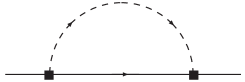
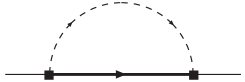
(a)                                     (b)

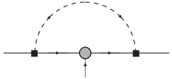
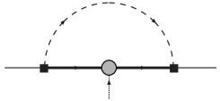
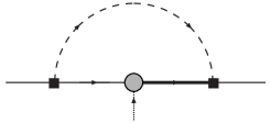
(c)                                     (d)                                     (e)

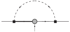
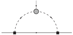
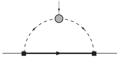
(f)                                    (g)                                     (h)
         
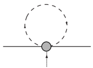
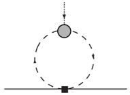
(i)                                      (j)

Figure 1: Diagrams contributing to nucleon matrix elements of the twist-two operators. The black square corresponds to an interaction from the strong Lagrangian and the gray circle represents an insertion of the twist-two operators in Eqs. (III.1)–(III.1). The thin, thick and dashed lines are 70–plet baryons, 44–plet baryons and mesons respectively. The first two diagrams represent the wave-function renormalisation and the remainder are operator renormalisations. Diagrams (e) and (f) are absent for the unpolarised, and isoscalar operator matrix elements, and diagrams in which the twist-two operator is inserted on a meson line are only present in the unpolarised case.

In Appendices B, C and D, we give the results for the independent matrix elements in SU(4$|$2) PQ$\chi$PT, for SU(6$|$3) PQ$\chi$PT and for SU(2$|$2) quenched  in the isospin limit. As an example, here we present the SU(4$|$2) isospin limit ($m_{u}=m_{d},\,m_{j}=m_{l}$), $q_{j}=q_{l}$ result for the nucleon matrix element of the isovector, unpolarised operators ${\cal O}_{\mu_{0}\ldots\mu_{n}}^{(3)}$:

$$\langle N|{\cal O}^{(3)}_{\mu_{0}\ldots\mu_{n}}|N\rangle = \frac{1}{3}{\overline{U}_{p}v_{\mu_{0}}\ldots v_{\mu_{n}}U_{p}}(2\alpha_{n}^{(a)}-\beta_{n}^{(a)})\times(1+(1-\delta_{n0}){\cal W}_{SU(4|2)})$$ (23)

$$+\frac{i(1-\delta_{n0})}{6f^{2}}\,{v_{\mu_{0}}\ldots v_{\mu_{n}}}\,\Bigg{\{}\frac{8}{3}\,g_{\Delta N}^{2}\,\left({{\gamma}_{n}^{(a)}}-\frac{{{\sigma}_{n}^{(a)}}}{3}\right)\Big{[}3\,{\cal H}({M_{\pi}},\Delta)\,+2\,{\cal H}({M_{uj}},\Delta)\,\Big{]}\,$$

$$\hskip 28.45274pt+{{\alpha}_{n}^{(a)}}\,\Bigg{[}8\,i\,{\cal I}({M_{uj}})\,-3\,{\cal H}({M_{uj}},0)\,\Big{[}2\,{g_{1}}\,{g_{A}}\,+3\,g_{1}^{2}\,\Big{]}+3{\cal H}({M_{\pi}},0)\,\Big{[}2\,g_{A}^{2}+2\,{g_{1}}\,{g_{A}}+3\,g_{1}^{2}\,\Big{]}$$

$$\hskip 85.35826pt+12\,{\delta}^{2}\,{\left({g_{1}}+{g_{A}}\right)}^{2}\,{{\cal H}_{\eta^{\prime}}}({M_{\pi}},0)\Bigg{]}$$

$$\hskip 28.45274pt-{{\beta}_{n}^{(a)}}\,\Bigg{[}4\,i\,{\cal I}({M_{uj}})\,-12{\cal H}({M_{uj}},0)\,{g_{1}}{g_{A}}+3{\cal H}({M_{\pi}},0)\,\left[4\,{g_{1}}\,{g_{A}}+g_{A}^{2}\right]$$

$$\hskip 85.35826pt+6\,{\delta}^{2}\,{\left({g_{1}}+{g_{A}}\right)}^{2}\,{{\cal H}_{\eta^{\prime}}}({M_{\pi}},0)\Bigg{]}\Bigg{\}},$$

where ${\mathcal{W}}_{\rm SU(4|2)}$ is the nucleon wave-function renormalisation given in Eq. (53) and

$$\delta^{2}=M_{\pi}^{2}-M_{uj}^{2}=\lambda(m_{u}-m_{j}),$$ (24)

is proportional to the difference between sea and valence quark masses. The functions ${\mathcal{I}}(M)$, ${\mathcal{H}}(M,\Delta)$ and ${\mathcal{H}}_{\eta^{\prime}}(M,\Delta)$ are defined in Eqs. (48), (33) and (34), below. Finally, $U_{B}$ corresponds to the type $B$ baryon spinor. To take the QCD limit, we would set $\delta\to 0$ and $j\to u$. For equivalent choices of the $\bar{\tau}_{A}$ our results reproduce those found previously for the unpolarised isovector operator Beane:2002vq ; Chen:2001yi . One can also calculate the matrix elements of these operators in the $\Delta$-isobar (and the N–$\Delta$ transition in the spin dependent cases). However since these are not stable particles in much of the region where  converges, we do not present the expressions.

In these results, the only effect of the diagrams in which the twist-two operator couples to a meson (diagrams (g), (h) and (j) in Fig. 1) is to satisfy the number sum rule for the $n=0$ matrix elements, producing the $\delta_{n0}$ factors in the above expression. For $n>0$, these diagrams give sub-leading contributions, entering at ${\cal O}(p^{n+2})$. The number sum-rule also fixes

$$2\alpha_{0}^{(a)}-\beta_{0}^{(a)}=3,\quad\quad\gamma_{0}^{(a)}=3,\quad\quad\sigma_{0}^{(a)}=0\,,$$

$$\alpha_{0}^{(s)}+\beta_{0}^{(s)}=3,\quad\quad\gamma_{0}^{(s)}=3,\quad\quad\sigma_{0}^{(s)}=0\,,$$ (25)

and the $n=0$ low energy constants of the spin-dependent operators can be fixed in terms of the usual axial couplings

$$2\Delta\alpha_{0}^{(a)}-\Delta\beta_{0}^{(a)}=6g_{A},\quad\quad\Delta\gamma_{0}^{(a)}=2g_{\Delta\Delta},\quad\quad\Delta\sigma_{0}^{(a)}=0,\quad\quad\Delta c_{0}^{(a)}=-\sqrt{\frac{3}{2}}g_{\Delta N}\,,$$

$$\Delta\alpha_{0}^{(s)}+\Delta\beta_{0}^{(s)}=2\left(g_{A}+g_{1}\right),\quad\quad\Delta\gamma_{0}^{(s)}=0,\quad\quad\Delta\sigma_{0}^{(s)}=0\,.$$ (26)

IV Finite volume corrections

IV.1 General discussion

In momentum space, the finite volume of a lattice simulation restricts the available momentum modes. Here we shall consider a hyper-cubic box of dimensions $L^{3}\times T$ with $T\gg L$. Imposing periodic boundary conditions on mesonic fields leads to quantised momenta $k=(k_{0},{\vec{k}})$, ${\vec{k}}=\frac{2\pi}{L}{\vec{j}}=\frac{2\pi}{L}(j_{1},j_{2},j_{3})$ with $j_{i}\in\mathbb{Z}$, but $k_{0}$ treated as continuous. On such a finite volume, spatial momentum integrals are replaced by sums over the available momentum modes. This leads to modifications of the infinite volume results presented in the previous section; the various functions arising from loop integrals are replaced by their FV counterparts. In a system where $M_{\pi}L\gg 1$, finite volume effects are predominantly from Goldstone mesons propagating to large distances where they are sensitive to boundary conditions and can even “wrap around the world”. Since the lowest momentum mode of the Goldstone propagator is $\sim\exp(-M_{\pi}L)$ in position space, finite volume effects will behave as a polynomial in $1/L$ times this exponential if no multi-particle thresholds are reached in the loop.

To investigate this behaviour, we consider the various finite volume sums occurring in the twist-two matrix elements. We first define

$$\frac{1}{L^{3}}\sum_{\vec{k}}\int dk_{0}\frac{k_{\mu}k_{\nu}}{(k^{2}-m^{2}+i\epsilon)(k\cdot v-\Delta+i\epsilon)}-\frac{ig_{\mu\nu}}{16\pi^{2}}\bar{\lambda}\left(\frac{2\Delta^{2}}{3}-m^{2}\right)\Delta$$

$$=g_{\mu\nu}{\mathcal{F}}(m,\Delta)+v_{\mu}v_{\nu}{\mathcal{G}}(m,\Delta)\,,$$ (27)

where the ultra-violet divergence has been subtracted in dimensional regularisation with $\bar{\lambda}=\frac{2}{4-d}-\gamma_{E}+{\mathrm{log}}(4\pi)+1$ ($d$ is the number of dimensions). All finite volume sums that occur in the baryon wave function and operator renormalisations involving baryon propagators (diagrams (a)–(h) in Fig. 1, sunset-type diagrams) can be expressed in terms of ${\mathcal{F}}(m,\Delta)$ and its derivatives. The tadpole diagrams in Fig. 1 are discussed in Appendix A. In the baryon rest frame where $v=(1,0,0,0)$, Poisson’s summation formula allows us to decompose ${\mathcal{F}}$ into its infinite-volume limit and a volume-dependent part,

$${\mathcal{F}}(m,\Delta)=F(m,\Delta)+F^{\mathrm{FV}}(m,\Delta)\,.$$ (28)

It is straightforward to show that the infinite volume piece is

$$F(m,\Delta)=\frac{i}{16\pi^{2}}\bigg{\{}\bigg{[}m^{2}-\frac{2\Delta^{2}}{3}\bigg{]}\,\Delta\,{\mathrm{log}}\left(\frac{m^{2}}{\mu^{2}}\right)+\bigg{[}\frac{10\Delta^{2}}{9}-\frac{4m^{2}}{3}\bigg{]}\,\Delta+\frac{2}{3}(\Delta^{2}-m^{2})^{3/2}\log\left(\frac{\Delta-\sqrt{\Delta^{2}-m^{2}+i\epsilon}}{\Delta+\sqrt{\Delta^{2}-m^{2}+i\epsilon}}\right)\bigg{\}}\,$$ (29)

($\mu$ is the renormalisation scale), and the finite volume corrections are given by

$$F^{\mathrm{FV}}(m,\Delta) = \frac{i}{12\pi^{2}}\sum_{\vec{u}\not=\vec{0}}\frac{1}{u\,L}\int_{0}^{\infty}d|\vec{k}|\,\frac{|\vec{k}|\,{\mathrm{sin}}(u|\vec{k}|L)}{\sqrt{|{\vec{k}}|^{2}+m^{2}}+\Delta}\left(\Delta+\frac{m^{2}}{\sqrt{|{\vec{k}}|^{2}+m^{2}}}\right)$$ (30)

$$\stackrel{{\scriptstyle mL\gg 1}}{{\longrightarrow}} \frac{i\,m^{2}}{24\pi}\sum_{\vec{u}\not=\vec{0}}\frac{{\mathrm{e}}^{-umL}}{u\,L}{\mathcal{A}}\,,$$

where $\vec{u}=(u_{1},u_{2},u_{3})$ with $u_{i}\in\mathbb{Z}$, $u\equiv|\vec{u}|$ and

$${\mathcal{A}} = {\mathrm{e}}^{(z^{2})}\big{[}1-{\mathrm{Erf}}(z)\mbox{ }\big{]}+\left(\frac{1}{umL}\right)\bigg{[}\frac{1}{\sqrt{\pi}}\left(\frac{9z}{4}-\frac{z^{3}}{2}\right)+\left(\frac{z^{4}}{2}-2\,z^{2}\right){\mathrm{e}}^{(z^{2})}\big{[}1-{\mathrm{Erf}}(z)\mbox{ }\big{]}\bigg{]}$$

$$-\left(\frac{1}{umL}\right)^{2}\bigg{[}\frac{1}{\sqrt{\pi}}\left(-\frac{39z}{64}+\frac{11z^{3}}{32}-\frac{9z^{5}}{16}+\frac{z^{7}}{8}\right)-\left(-\frac{z^{6}}{2}+\frac{z^{8}}{8}\right){\mathrm{e}}^{(z^{2})}\big{[}1-{\mathrm{Erf}}(z)\mbox{ }\big{]}\bigg{]}+{\mathcal{O}}\left(\frac{1}{(umL)^{3}}\right),$$

with

$$z=\left(\frac{\Delta}{m}\right)\sqrt{\frac{umL}{2}}.$$ (32)

Higher order terms in the $1/(umL)$ expansion in Eq. (IV.1) are easily calculated. For convenience, we also define the functions

$${\mathcal{H}}(m,\Delta)\equiv\frac{\partial{\mathcal{F}}(m,\Delta)}{\partial\Delta}\qquad{\rm and}\qquad{\mathcal{K}}(m,\Delta)\equiv\frac{{\mathcal{F}}(m,\Delta)-{\mathcal{F}}(m,0)}{\Delta}\,,$$ (33)

and their finite volume counterparts which we denote by the corresponding roman letter with the superscript ^FV as in Eq. (28), e.g. ${\mathcal{K}}\to K^{\rm FV}$.

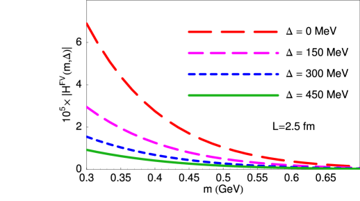
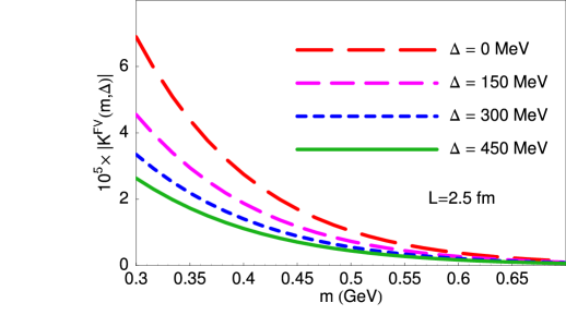
Figure 2: Dependence of finite volume effects on the mass-splitting $\Delta$ in individual integrals/sums corresponding to diagrams (a)—(f) in Fig. 1. The point $m=0.3$ GeV corresponds to $mL=3.8$.

The function $\cal A$ represents the modification of the FV effects due to the mass-splitting $\Delta$; in the limit $\Delta\to 0$, ${\cal A}\to 1$. Figure 2 shows the dependence of FV effects on the scale $\Delta$ for the functions $H^{\rm FV}(m,\Delta)$ and $K^{\rm FV}(m,\Delta)$ that arise from diagrams (a)—(f) in Fig. 1. It is clear that finite volume effects in individual diagrams involving a 44-plet are suppressed relative to those involving only meson and 70-plet baryon propagators, though this can be compensated for by large coefficients. A very similar result was found in the heavy meson sector Arndt:2004bg where the contributions involving $B^{*}$ mesons are suppressed compared to those involving the $B$ meson by the mass difference $\Delta_{B}=m_{B^{*}}-m_{B}$. However, the origin and behaviour of the mass difference in the current context is distinct. In contrast to the heavy meson case where $\Delta_{B}\sim 1/m_{B}$ arises from the breaking of heavy-quark spin symmetry and vanishes in the heavy quark limit, the mass difference $\Delta$ is generated by strong-interaction dynamics and remains finite in the chiral limit. Empirically, $\Delta$ is almost constant over the range of quark masses considered here.

When one considers quenched or partially quenched theories rather than standard , one expects somewhat larger finite volume effects because of the enhanced long-distance behaviour of double-pole structures in the singlet meson propagators of these theories Bernard:1995ez . These double pole contributions are given by terms proportional to the functions

$${\mathcal{H}}_{\eta^{\prime}}(m,\Delta)\equiv\frac{\partial{\mathcal{H}}(m,\Delta)}{\partial m^{2}}\,,\qquad\qquad\qquad{\mathcal{K}}_{\eta^{\prime}}(m,\Delta)\equiv\frac{\partial{\mathcal{K}}(m,\Delta)}{\partial m^{2}}\,,$$ (34)

and the double-pole tadpole function ${\mathcal{I}}_{\eta^{\prime}}(m)$ given in Appendix A [and their finite volume analogues constructed as in Eq. (28)]. From Figures 2 and 3 it is clear that $H^{\rm FV}_{\eta^{\prime}}(m,\Delta)$ is about an order of magnitude larger than $H^{\rm FV}(m,\Delta)$ in accordance with expectations.

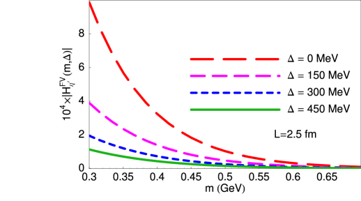
Figure 3: Dependence of finite volume effects in double-pole contributions on the mass-splitting $\Delta$. Note that the scale here is ten times that in Fig. 2. The point $m=0.3$ GeV corresponds to $mL=3.8$.

In considering the magnitude of finite volume effects, the standard chiral power counting can be misleading; the FV effects of a diagram of a given order in the power counting may be larger than those of lower orders. For some generic observable, one may consider two contributions, ${\cal C}_{1}$ and ${\cal C}_{2}$, that enter at different orders, $m_{1}<m_{2}$, in infinite volume . As discussed above, the dominant finite volume effects in these contributions will typically be of the form $\delta{\cal C}_{i}\sim(M_{\pi}L)^{\ell_{i}}\exp(-M_{\pi}L)$ when $M_{\pi}L\gg 1$ and no multi-particle on-shell intermediate states can contribute. In some situations, the presence of additional meson propagators or other infrared enhancement in the higher order contribution (${\cal C}_{2}$) can amplify its finite volume shift relative to that of the lower order contribution (${\cal C}_{1}$). For some (contemporarily relevant) choices of masses and volumes, the quantity

$$(M_{\pi}L)^{\ell_{2}-\ell_{1}}\left(\frac{M_{\pi}}{\Lambda_{\chi}}\right)^{m_{2}-m_{1}}>1\,,$$ (35)

and the formally higher-order contribution will provide the dominant finite volume effect. In the current calculation, diagram (g) in Fig. 1, in which the twist-two operator is attached to mesonic propagators, may indeed fall into such a category. The finite volume corrections to these diagrams will be given by

$$\delta I_{\pi}^{(n)}\sim a^{(a)}_{n}\frac{1}{\Lambda_{\chi}^{n}}\frac{M_{\pi}^{n+1}}{4f^{2}}\frac{\partial}{\partial M_{\pi}^{2}}F^{\rm FV}(M_{\pi},0)\,,$$ (36)

compared with those of the corresponding baryon operator diagrams (diagram (c) in Fig. 1)

$$\delta I_{N}^{(n)}\sim\frac{\alpha_{n}^{(a)}}{f^{2}}H^{\rm FV}(M_{\pi},0)\,.$$ (37)

From this we see that the ratio

$$\frac{\delta I_{\pi}^{(n)}}{\delta I_{N}^{(n)}}\sim\left(\frac{M_{\pi}}{\Lambda_{\chi}}\right)^{n}\frac{1}{4\sqrt{M_{\pi}L}}\left(1-\frac{M_{\pi}\,L}{2}\right)\,,$$ (38)

where there is an undetermined coefficient involving $a_{n}^{(a)}$, $\alpha_{n}^{(a)}$ and other numerical factors that we assume to be ${\cal O}(1)$. Whilst formally the magnitude of this ratio is indeed greater than unity for any $n$ in the limit $M_{\pi}\,L\to\infty$, both $\delta I_{\pi}^{(n)}$ and $\delta I_{N}^{(n)}$ are exponentially suppressed. For realistic pion masses and volumes used in current lattice simulations this ratio is consistently smaller than one and the FV effects of diagrams (g), (h) and (j) in Fig. 1 can be neglected. The only exception to this is in the $n=0$ unpolarised matrix elements, the isoscalar and isovector quark numbers. Here, the volume dependence of diagrams in Fig. 1 with mesonic operators exactly cancels that of those involving baryonic operators and wave-function renormalisations to give an overall result that is independent of the volume.

IV.2 Relevance to lattice data

Lattice calculations of twist-two matrix elements have a long history, with the first calculations occurring in the 1980s Martinelli:1987si . Over the last decade, a considerable effort has been made to study them in detail with major contributions from the QCDSF, LHP, RBCK and ZeRo collaborations. In Table 1, recent simulation parameters are shown. State-of-the-art lattice simulations are beginning to enter the region of quark masses and lattice volumes in which the use of NLO chiral perturbation theory is justified (naively, this requires $m_{\pi}/\Lambda_{\chi}\lesssim 1/3$ and $m_{\pi}L\gtrsim 4$). At the moment however, there is little data in this region and a realistic fit of the combined mass and volume dependence in our PQ$\chi$PT formulae (and thereby a determination of the LECs) is not possible; only general trends can be extracted.

Group	$m_{\pi}$ [MeV]	Volume [fm3]	Notes
Dynamical simulations ($N_{f}=2$)
QCDSF Gockeler:2004vx	560–940	1.13, 1.53, 2.23	Clover, a$\sim$0.08–0.12 fm
LHP Renner:2004ck	340	3.53	Staggered sea, DW valence, a$\sim$0.13 fm
LHP Renner:2004ck	340–730	2.63	Staggered sea, DW valence, a$\sim$0.13 fm
LHP-SESAM Dolgov:2002zm	730–900	1.63	Wilson, a$\sim$0.1 fm
LHP-SCRI Dolgov:2002zm	480–670	1.53	Wilson, a$\sim$0.1 fm
RBCK Ohta:2004mg	560–700	1.93	DW, a$\sim$0.13 fm
Quenched simulations
QCDSF Gockeler:2004wp	580–1200	1.63	Clover, a$\sim$0.05, 0.07, 0.09 fm
QCDSF Gockeler:1995wg	310–1000	1.53	Wilson, a$\sim$0.09 fm
QCDSF Gurtler:2004ac	440–950	1.53, 2.33	Overlap, a$\sim$0.095 fm
LHP Dolgov:2002zm	580–820	1.63	Wilson,a$\sim$0.1 fm
RBCK Sasaki:2003jh	390–850	1.23,1.63,2.43	DW, a$\sim$0.15 fm
ZeRo Wetzorke:2004xv	750–910	1.13,1.53,2.23,3.03	Clover, a$\sim$0.093 fm

Table 1: Summary of recent lattice calculations of nucleon twist two matrix elements. Not all calculations involve the full set of twist-two operators.

In order to address the expected size of finite volume corrections arising from our calculation, we first define the finite volume correction

$$\langle N|{\cal O}|N\rangle^{\rm FV}=\frac{\langle N|{\cal O}|N\rangle_{L}^{\rm one-loop}-\langle N|{\cal O}|N\rangle_{L=\infty}^{\rm one-loop}}{\langle N|{\cal O}|N\rangle^{\rm tree-level}}\,,$$ (39)

for each of the operator matrix elements we calculate. These corrections depend on a number of low-energy constants and couplings, some of which involve the $\Delta$ resonance. In principle, all of these parameters can be extracted from fits of the  forms to lattice data on nucleon matrix elements (thereby bypassing issues of the structure of unstable particles and transition matrix elements), however this is not practical at the present stage. Therefore, to fix the twist-two low energy constants ($\alpha_{n}^{(a)}$, $\delta\gamma_{n}$ etc) we assume that large-$N_{c}$ relations Chen:2001et amongst the parton distributions in the nucleon, $\Delta$-isobar and $N$–$\Delta$ transition are valid, leading to

$$\gamma_{n}^{(a)} =2\alpha_{n}^{(a)}-\beta_{n}^{(a)}\,,\qquad\qquad\Delta\gamma_{n}^{(a)} =\frac{1}{5}\left(2\Delta\alpha_{n}^{(a)}-\Delta\beta_{n}^{(a)}\right)\,,\qquad\Delta c_{n}^{(a)}=\frac{1}{2}\left(2\Delta\alpha_{n}^{(a)}-\Delta\beta_{n}^{(a)}\right)\,,$$ (40)

$$\gamma_{n}^{(s)} =\alpha_{n}^{(s)}+\beta_{n}^{(s)}\,,\qquad\qquad\Delta\gamma_{n}^{(s)} =\Delta\alpha_{n}^{(s)}+\Delta\beta_{n}^{(s)}\,,\qquad\qquad\quad\delta\alpha_{n}=-4\delta\beta_{n}=\frac{4}{5}\delta\gamma_{n}=\frac{8}{9}\delta c_{n}\,.$$

The remaining LECs are not constrained by large-$N_{c}$ relations in QCD, and for want of accurate lattice data with which to fit them, we set $\beta_{n}^{(a,s)}=\alpha_{n}^{(a,s)}$, $\Delta\beta_{n}^{(a,s)}=\Delta\alpha_{n}^{(a,s)}$ and $\sigma_{n}^{(a,s)}=\Delta\sigma_{n}^{(a,s)}=\delta\sigma_{n}=0$. Throughout, we use $f=0.132$ GeV, and keep $\Delta=0.3$ GeV fixed independent of the quark mass. For the parameters appearing in the the flavour matrices $\bar{\tau}_{3}$ and $\bar{\tau}_{T}$, we set $q_{j}=q_{l}=q_{k}=0$ and $y_{j}=y_{k}=y_{l}=y_{m}=0$, and set $y_{i}$ to be either $\pm 1$. As discussed above, if one is using lattice data to determine the LECs, the $q$’s and $y$’s are fixed by the details of the lattice calculation. After making all of the above substitutions, the isospin limit results become proportional to the corresponding bare matrix elements and the finite volume effects given by Eq. (39) are easily studied.

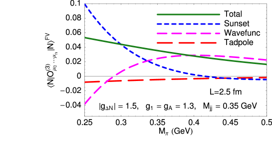
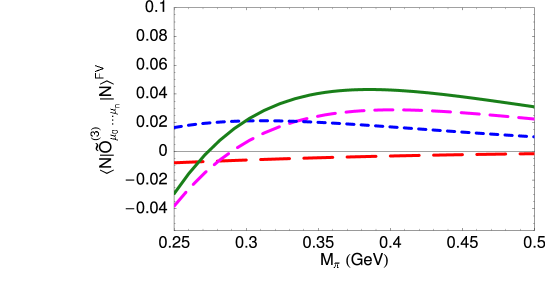
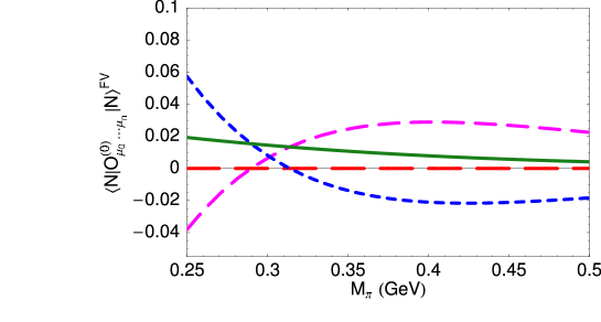
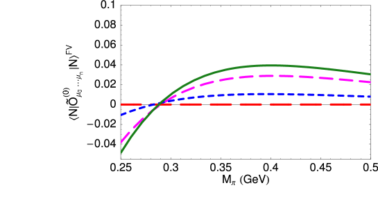
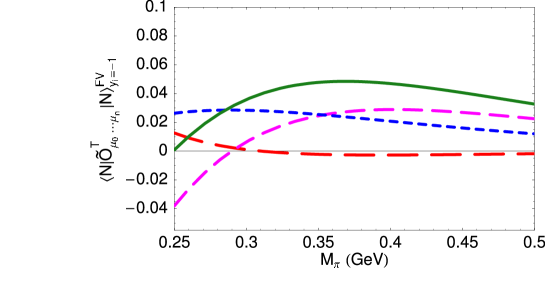
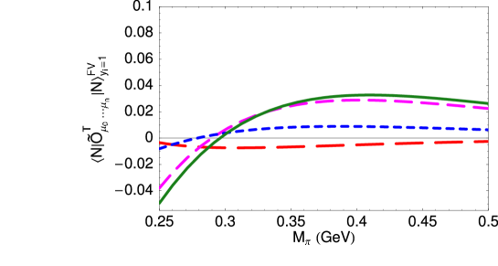
Figure 4: Indicative finite volume effects in SU(4$|$2) matrix elements. The results in the first row are for the isovector unpolarised (left) and helicity (right) operators and those in the second row are similarly for the isoscalar unpolarised (left) and helicity (right) operators. The third row corresponds to the transversity “isovector” $y_{i}=-1$ (left) and “isoscalar” $y_{i}=1$ (right) matrix elements. In each plot, the solid curve shows the total result, whilst the short-, medium- and long-dashed curves correspond to the individual FV effects arising from diagrams (c)–(f), diagrams (a) and (b), and diagram (i) in Fig.  1. In all of these results, we have considered a (2.5 fm)³ box and set $g_{A}=g_{1}=1.3$ and $|g_{\Delta N}|=1.5$. $M_{\pi}=0.25$ GeV corresponds to $M_{\pi}L=3.2$.

The axial couplings $g_{A}$, $g_{1}$, and $g_{\Delta N}$ occurring in our results are the chiral limit couplings and there is some uncertainty in their values. We will fix $g_{A}=1.3$ (though even the chiral limit value of this is not well known Beane:2004ks ), $|g_{\Delta N}|=1.5$ and vary $g_{1}=\pm g_{A}$. In the QCD limit, results are independent of $g_{1}$ since in this case it only involves couplings to the $\eta^{\prime}$ meson which remains massive in the chiral limit and can be integrated out.

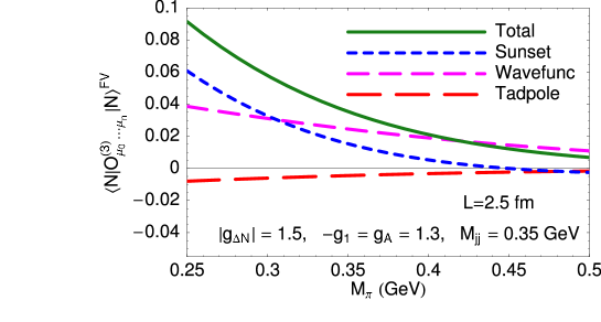
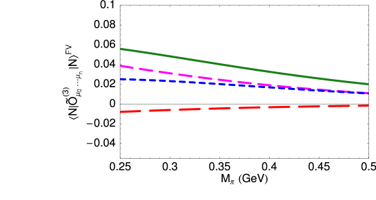
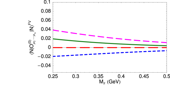
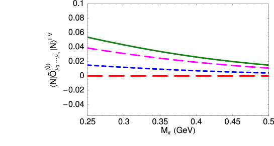
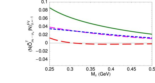
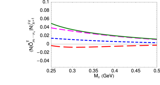
Figure 5: As in Fig. 4 except with $g_{1}=-g_{A}$. $M_{\pi}=0.25$ GeV corresponds to $M_{\pi}L=3.2$.

Using these parameters, Figures 4 and 5 illustrate the typical size of finite volume effects in the various matrix elements. In Fig. 4, we consider a (2.5 fm)³ box with a sea quark mass set such that the corresponding sea–sea Goldstone boson has a mass $M_{jj}=0.35$ GeV and take $g_{1}=g_{A}$. Fig. 5 is similar except here we take $g_{1}=-g_{A}$ to show the effect of this undetermined parameter. Variation of $g_{A}$ and $g_{\Delta N}$ within reasonable bounds leads to similar modifications as those for varying $g_{1}$. At the smallest pion mass in these plots, $M_{\pi}L\sim 3$ and one must start to worry that infinite volume $p$-counting is no longer appropriate; at the largest pion mass in the plots, $M_{\pi}/\Lambda_{\chi}\sim 1/2$ and one must worry that the convergence of the chiral expansion becomes questionable. From these figures, it is nevertheless apparent that NLO PQ$\chi$PT predicts finite volume effects in twist-two matrix elements that are generically $\lesssim 5$–10% for the range of masses and volumes studied here. However, there is some evidence that finite volume effects from higher orders of the standard chiral power-counting can be significant Colangelo:2003hf ; Colangelo:2004xr .

Recently, staggered-sea, domain-wall-valence results have become available from the LHP collaboration Renner:2004ck for very large volume ($L=3.5$ fm) calculations of $g_{A}$ at a pion mass of 337 MeV. Also available are results on a somewhat smaller lattice ($L=2.6$ fm) at the same pion mass. Although these two data points are consistent within their statistical errors (which will be reduced by ongoing calculations), their central values differ by $\sim 15$%. If we ignore the issues of non-locality due to the “fourth-root” trick used in calculating the staggered quark configurations and possible unitarity violations arising from the different valence and sea quark actions (which must vanish in the $a\to 0$ limit that we have assumed), one can ask whether the NLO PQ$\chi$PT formulae presented here can describe this dependence. To address this question, we consider the isospin symmetric QCD limit ($m_{u}=m_{d}=m_{j}=m_{l}$) and define

$$\delta g_{A}=\frac{\langle N|\widetilde{\cal O}^{(3)}_{\mu}|N\rangle_{L}^{\rm one-loop}-\langle N|\widetilde{\cal O}^{(3)}_{\mu}|N\rangle_{L=\infty}^{\rm one-loop}}{\langle N|\widetilde{\cal O}^{(3)}_{\mu}|N\rangle^{\rm tree-level}}\,.$$ (41)

For this case, the LECs can be expressed in terms of the axial couplings through Eq. (26) and the FV shift, $\delta g_{A}$, depends only on the pion mass, the volume and the chiral limit couplings $g_{A}$, $g_{\Delta N}$ and $g_{\Delta\Delta}$. In Fig. 6, we show the FV shift in $g_{A}$ that NLO  predicts at the LHP pion mass, $M_{\pi}=337$ MeV. To illustrate uncertainties in the results, we vary the different axial couplings. In the central fits (indicated by the curves in the plot), we set $g_{A}=1.3$, $g_{\Delta N}=-1$ and $g_{\Delta\Delta}=-3$ whilst the shaded band corresponds to $\delta g_{A}$ for $1.0\leq g_{A}\leq 1.5$, $0\leq|g_{\Delta N}|\leq 2$ and $g_{\Delta\Delta}=-3$. Whilst, a shift of 15% between $L=2.6$ and 3.5 fm is not predicted, the FV effects are substantial. However, without accurate knowledge of the chiral limit couplings, even the sign of the finite volume correction to $g_{A}$ is not well determined.

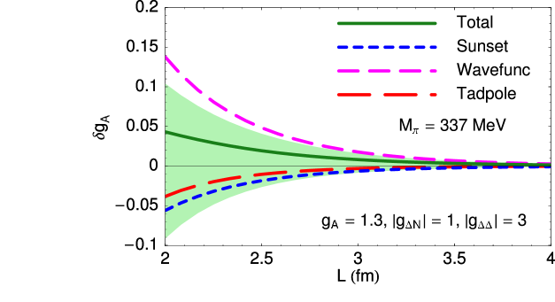
Figure 6: Finite volume effects in QCD calculations of $g_{A}$ at $M_{\pi}=337$ MeV (as appropriate for the recent LHP simulations Renner:2004ck ). $L=2$ fm corresponds to $M_{\pi}L=3.4$. The shaded region corresponds to varying $1.0\leq g_{A}\leq 1.5$, $0\leq|g_{\Delta N}|\leq 2$.

As discussed in the previous subsection, in quenched lattice calculations, FV effects will be enhanced because of the double-pole contributions to singlet meson propagators. In Fig. 7, we plot the volume dependence of the polarised, isovector twist-two matrix elements in SU(2$|$2) quenched  (the analytic forms of these results are presented in Appendix D). In contrast to partially-quenched , in the quenched theory the LECs occurring in the Lagrangian and the twist-two operators are unrelated to those in standard (though we denote them by the same symbols for convenience). To be definite, we choose $m_{0}=0.7$ GeV and the quenched operator LECs to satisfy $\Delta\alpha^{(a)}_{n}=\Delta\beta^{(a)}_{n}=5\Delta\gamma^{(a)}_{n}=2\Delta c_{n}^{(a)}$ (as in the partially-quenched case), set the quenched axial couplings to $g_{A}=1.3$, $|g_{\Delta N}|=1.5$ and let $g_{1}$ and $\gamma$ vary between $\pm g_{A}$ as indicated by the shaded region. The curves in the figure correspond to $g_{1}=g_{A}/2$ and $\gamma=0$. As expected, the volume dependence here is enhanced over that in the PQ$\chi$PT and  cases.

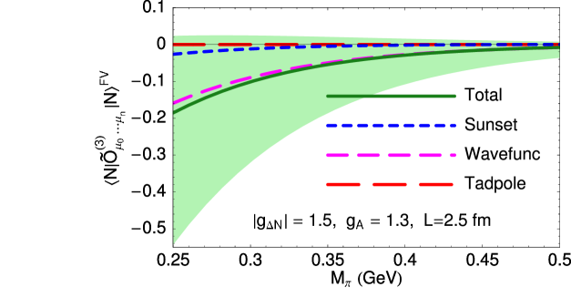
Figure 7: Finite volume effects in the isovector, helicity matrix elements in the proton in SU(2$|$2) quenched . The shaded region corresponds to variation of the axial couplings $g_{1}$ and $\gamma$ between $\pm g_{A}$ with $g_{A}=1.3$, $g_{\Delta N}=1.5$ and assuming large $N_{c}$ relations for the operator LECs. The point $M_{\pi}=0.25$ GeV corresponds to $M_{\pi}L=3.2$.

IV.3 Off-forward matrix-elements

The off-forward matrix elements (in which the incoming and outgoing hadrons carry different momenta) of the twist-two operators correspond to moments of generalised parton distributions. Very little is known from experiment about GPDs though major programs are underway at HERMES, Jefferson Lab and COMPASS to investigate them. As such, moments of GPDs are important quantities to extract from lattice calculations and much progress is being made in this direction latticeGPDs . It is therefore important to investigate the quark mass dependence and size of finite volume effects in these calculations. Here we shall only discuss the novel features that appear in regard to finite volume effects when off-forward matrix elements are considered. A full analysis of the low-energy behaviour of these matrix elements will be given elsewhere offforward .

To be specific, we shall consider the proton matrix elements $\langle p^{\prime}|^{\rm QCD}{\cal O}_{\mu_{0}\ldots\mu_{n}}^{(A)}|p\rangle$ in which four momentum $q^{\mu}=(p^{\prime}-p)^{\mu}$ (with $|q^{2}|\ll\Lambda_{\chi}^{2}$) is injected through the twist-two operator. The analysis of these matrix elements is significantly more complicated than in the forward limit. This is primarily because the number of possible independent tensor structures in the matrix element grows with $n$; for example,

$$\langle p^{\prime}|^{\rm QCD}{\cal O}_{\mu_{0}\ldots\mu_{n}}^{(A)}|p\rangle = \overline{U}_{p}(p^{\prime})\Bigg{[}\sum_{\begin{subarray}{c}i=0\\ {\rm even}\end{subarray}}^{n}\Bigg{\{}\gamma^{\{\mu_{0}}q^{\mu_{1}}\ldots q^{\mu_{i}}{\bar{p}}^{\mu_{i+1}}\ldots{\bar{p}}^{\mu_{n}\}}A^{(A)}_{n,i}(q^{2})$$

$$-i\frac{q_{\nu}\sigma^{\nu\{\mu_{0}}}{2m}q^{\mu_{1}}\ldots q^{\mu_{i-1}}{\bar{p}}^{\mu_{i}}\ldots{\bar{p}}^{\mu_{n}\}}B^{(A)}_{n,i}(q^{2})\Bigg{\}}+\left.\frac{q^{\mu_{0}}\ldots q^{\mu_{n}}}{m}C^{(A)}_{n,0}(q^{2})\right|_{n\text{ even}}\Bigg{]}U_{p}(p)\,,$$

where ${\bar{p}}=\frac{1}{2}(p^{\prime}+p)$. For each of the coefficient functions $A^{(A)}_{n,i}(q^{2})$, $B^{(A)}_{n,i}(q^{2})$ and $C^{(A)}_{n,0}(q^{2})$, there is an independent finite volume  expansion.

Another complication enters when one considers the operators that match onto the twist-two operators in the low energy effective theory. The presence of the new scale $q$ means that considerably more operators must be included in Eqs. (III.1)–(III.1); for example, the term proportional to $\alpha^{(r_{A})}_{n}$ in Eq. (III.1) is replaced by

$$\Bigg{[}\sum_{j=0}^{n}\alpha^{(r_{A})}_{n,j}\left[v^{\{\mu_{0}}\ldots v^{\mu_{j}}(-i\partial)^{\mu_{j+1}}\ldots(-i\partial)^{\mu_{n}\}}-{\rm tr}\right]+\alpha^{(r_{A})}_{n,-1}\left[(-i\partial)^{\mu_{0}}\ldots(-i\partial)^{\mu_{n}}-{\rm tr}\right]\Bigg{]}(\overline{\cal B}\tau^{A}_{\xi^{+}}{\cal B})\,.$$ (43)

Note that only terms with an even number of derivatives contribute here. Each LEC in the forward case is replaced by ${\cal O}(n)$ LECs. Additionally, the vector $q$ allows more tensor structures to enter and we must also include

$$\sum_{j=0}^{n}\hat{\alpha}^{(r_{A})}_{n,j}\left[v^{\{\mu_{0}}\ldots v^{\mu_{j}}(-i\partial)^{\mu_{j+1}}\ldots(-i\partial)^{\mu_{n-1}}(\overline{\cal B}\frac{\left[S_{\mu_{n}\}},S\cdot(-i\partial)\right]}{M}\tau^{A}_{\xi^{+}}{\cal B})-{\rm tr}\right]\,,$$ (44)

since $S\cdot q\neq 0$. When we also take into account the 44-plet fields ${\cal T}^{\mu}$, many more structures are possible since $q\cdot{\cal T}\neq 0$. Even for the $n<3$ matrix elements that have been calculated on the lattice, a large number of LECs need to be determined. This makes a reliable extraction of the physical matrix elements from finite volume, unphysical mass, lattice calculations a challenging proposition.

In terms of FV effects, the modifications for the off-forward case are relatively simple and it is worthwhile to investigate them in some detail. There are essentially two classes of diagrams: ones where the twist-two operator injects momentum into a (heavy) baryon field (e.g., (c) in Fig. 1); and ones where a meson receives the additional momentum (e.g., (h) in Fig. 1). The former class is relatively uninteresting since for heavy fields, derivatives in the twist-two operators pick out only the momentum transfer between the external states, $q$, and can therefore be factored out of the integral. For this type of diagram, finite volume effects will be the same as those in the forward limit as we are free to work in the Breit frame where $q\cdot v=0$.

For diagrams in which the twist-two operator is on a meson line, the situation is different since the derivatives in the operator can result in powers of the integration momentum. The relevant integrals are of the form

$$\frac{1}{L^{3}}\sum_{\vec{k}}\int\frac{dk_{0}}{2\pi}\frac{S\cdot(-k)S\cdot(k+q)\left[(-k)^{\{\mu_{0}}\ldots(-k)^{\mu_{j}}(k+q)^{\mu_{j+1}}\ldots(k+q)^{\mu_{n}\}}-{\rm tr}\right]}{(k\cdot v-\Delta+i\epsilon)\,(k^{2}-m^{2}+i\epsilon)((k+q)^{2}-m^{2}+i\epsilon)}\hskip 133.72786pt$$ (45)

$$\hskip 15.6491pt=4\int_{0}^{1}dx\int_{0}^{\infty}d\lambda\frac{1}{L^{3}}\sum_{\vec{\ell}}\int\frac{d\,\ell_{0}}{2\pi}\frac{S\cdot(\ell+a)S\cdot(\ell+b)}{(\ell^{2}-{\cal M}^{2})^{3}}(-1)^{j}\left[(\ell+a)^{\{\mu_{0}}\ldots(\ell+a)^{\mu_{j}}(\ell+b)^{\mu_{j+1}}\ldots(\ell+b)^{\mu_{n}\}}-{\rm tr}\right]$$

after introducing Feynman and Schwinger parameters and shifting the momentum integration $k\to\ell=k+x\,q-\lambda\,v$. Here $a=-x\,q+\lambda\,v$, $b=(1-x)\,q+\lambda\,v$ and

$${\cal M}^{2}\equiv{\cal M}^{2}(x,\lambda,m^{2},q^{2},\Delta)=m^{2}-x(1-x)q^{2}+\lambda^{2}+2\lambda\Delta\,.$$ (46)

The trace subtractions prevent any of the $\ell^{\mu_{i}}$’s arising from the operator from contracting with one another, consequently the non-vanishing scalar integrals/sums whose finite volume effects we are interested in will be of the form

$$\int_{0}^{1}dx\int_{0}^{\infty}d\lambda\frac{1}{L^{3}}\sum_{\vec{\ell}}\int\frac{d\,\ell_{0}}{2\pi}\frac{\left(\ell^{2}\right)^{r}}{(\ell^{2}-{\cal M}^{2})^{3}}\,,$$ (47)

where $r=0$, 1 or 2.

Without going into further details of the tensor structure offforward , it is already clear from Eq. (46) that the effect of the momentum injection on overall finite volume shifts is very similar to the effect of the N–$\Delta$ mass splitting. Since $x(1-x)>0$, when space-like momentum ($q^{2}=-|{\vec{q}}|^{2}<0$ in Minkowski space) is injected, FV effects are suppressed as the meson receiving the momentum injection moves further away from its mass shell. However, if time-like momentum is injected the situation is more complicated. Provided the virtual particle cannot reach its mass shell, finite volume effects are enhanced over the forward case but will still remain formally exponentially suppressed. However, if the injected energy-momentum is enough to put the intermediate particles on shell, it leads to a cut in Minkowski space in infinite volume. In this case, finite volume effects are only suppressed by powers of $1/L$ in QCD. In (partially) quenched QCD, volume corrections for isoscalar twist-two matrix elements may be proportional to positive powers of $L$ whereby the infinite volume limit will be undefined. This suppression of finite volume effects with space-like momentum injection and enhancement in the time-like case (which is relevant for twist-two matrix elements between states of different masses, e.g. $N\to\Delta$ transitions) will occur in hadronic form-factors that are specific cases of twist-two matrix elements.

V Conclusions

We have studied the matrix elements of twist-two operators that determine the moments of the unpolarised, helicity and transversity quark distributions to NLO in (partially) quenched chiral perturbation theory in both infinite and finite volumes. We have performed our calculations in $N_{f}=2$ and $N_{f}=2+1$ partially quenched heavy baryon chiral perturbation theory and also studied the SU(2$|$2) quenched theory. These results will be relevant for extrapolations of lattice calculations of these matrix elements in the proton and other octet baryons (e.g., the $\Lambda$ hyperon Gockeler:2002uh ).

We have focused primarily on the effects of the finite volumes used in lattice calculations. Without accurate data in the chiral regime with which to fit the various low energy constants on which the results depend, it is difficult to be specific, however it is clear that for most current simulations FV effects are not negligible. For typical full- or partially-quenched- QCD calculations, they are $\lesssim 5$–10% but may be significantly larger in quenched simulations.

In the case of the off-forward matrix elements relevant to generalised parton distributions, we have not presented full results for arbitrary moments offforward . However, we have analysed the finite volume effects in these matrix elements. We find that they should decrease with respect to the forward matrix elements if space-like momentum is injected. On the other hand if time-like momentum is transferred, finite volume effects will be enhanced; in QCD they may become only $1/L$ suppressed, and in (partially) quenched QCD finite volume isoscalar matrix elements may even be proportional to powers of $L$.

Appendix A Tadpole integrals and finite volume sums

The sums that appear in tadpole diagrams, after subtracting $\bar{\lambda}$, are

$${\mathcal{I}}(m) = \frac{1}{L^{3}}\sum_{\vec{k}}\int\frac{dk_{0}}{2\pi}\frac{i}{k^{2}-m^{2}+i\epsilon}+\frac{m^{2}}{16\pi^{2}}\bar{\lambda}\,,$$ (48)

and

$${\mathcal{I}}_{\eta^{\prime}}(m) = \frac{1}{L^{3}}\sum_{\vec{k}}\int\frac{dk_{0}}{2\pi}\frac{i}{(k^{2}-m^{2}+i\epsilon)^{2}}+\frac{1}{16\pi^{2}}\bar{\lambda}=\frac{\partial{\mathcal{I}}(m)}{\partial m^{2}}.$$ (49)

Using Poisson’s summation formula, it is straightforward to show that

$${\mathcal{I}}(m)=I(m)+I^{\mathrm{FV}}(m),$$ (50)

where

$$I(m)=\mu^{4-d}\int\frac{d^{d}k}{(2\pi)^{d}}\frac{i}{k^{2}-m^{2}+i\epsilon}+\frac{m^{2}}{16\pi^{2}}\bar{\lambda}=\frac{m^{2}}{16\pi^{2}}{\mathrm{log}}\left(\frac{m^{2}}{\mu^{2}}\right),$$ (51)

is the infinite-volume limit of ${\mathcal{I}}(m)$, and

$$I^{\mathrm{FV}}(m) = \frac{m}{4\pi^{2}}\sum_{\vec{u}\not=\vec{0}}\frac{1}{uL}K_{1}(umL)$$ (52)

$$\stackrel{{\scriptstyle mL\gg 1}}{{\longrightarrow}} \frac{1}{4\pi^{2}}\sum_{\vec{u}\not=\vec{0}}\sqrt{\frac{m\pi}{2uL}}\left(\frac{1}{uL}\right){\mathrm{e}}^{-umL}\left\{1+\frac{3}{8umL}-\frac{15}{128(umL)^{2}}+{\mathcal{O}}\left(\frac{1}{(umL)^{3}}\right)\right\}\,.$$

Appendix B Results for SU(4$|$2) PQ$\chi$PT

In this section, we present the results for twist-two matrix elements in the isospin limit in $SU(4|2)$ PQ$\chi$PT. The various masses and the mass-splitting $\delta$ are defined in Sections II and  III.

The nucleon wave-function renormalisation is

$${\cal W}_{SU(4|2)} = \frac{i}{2f^{2}}\Big{\{}{\cal H}({M_{\pi}},0)\,\left(-5\,g_{1}^{2}-4\,{g_{1}}\,{g_{A}}+g_{A}^{2}\right)+{\cal H}({M_{uj}},0)\,\left(5\,g_{1}^{2}+4\,{g_{1}}\,{g_{A}}+8\,g_{A}^{2}\right)$$ (53)

$$+4\,\left({\cal H}({M_{\pi}},\Delta)+{\cal H}({M_{uj}},\Delta)\right)\,g_{\Delta N}^{2}+\left(-6\,\,g_{1}^{2}-12\,\,{g_{1}}\,{g_{A}}-6\,\,g_{A}^{2}\right){\delta}^{2}\,{{\cal H}_{\eta^{\prime}}}({M_{\pi}},0)\big{\}}\,.$$

The isovector, unpolarised nucleon matrix element is

$$\langle N|{\cal O}^{(3)}_{\mu_{0}\ldots\mu_{n}}|N\rangle = \frac{1}{3}{\overline{U}_{N}v_{\mu_{0}}\ldots v_{\mu_{n}}}U_{N}(2\alpha_{n}^{(a)}-\beta_{n}^{(a)})\times(1+(1-\delta_{n0}){\cal W}_{SU(4|2)})$$ (54)

$$+\frac{i(1-\delta_{n0})}{12f^{2}}\,{\overline{U}_{N}v_{\mu_{0}}\ldots v_{\mu_{n}}U_{N}}\,\Bigg{\{}\frac{4}{3}\,g_{\Delta N}^{2}\,\left({{\gamma}_{n}^{(a)}}-\frac{{{\sigma}_{n}^{(a)}}}{3}\right)\times\$$

$$\hskip 42.67912pt\Bigg{[}-3\,{\cal H}({M_{\pi}},\Delta)\,\left(-4+{q_{j}}+{q_{l}}\right)+{\cal H}({M_{uj}},\Delta)\,\left(8+3\,{q_{j}}+3\,{q_{l}}\right)\Bigg{]}\,$$

$$+{{\alpha}_{n}^{(a)}}\,\Bigg{[}-4\,i\,{\cal I}({M_{uj}})\,\left(-4+3\,{q_{j}}+3\,{q_{l}}\right)+4\,i\,{\cal I}({M_{\pi}})\,\left({q_{j}}+{q_{l}}\right)$$

$$\hskip 28.45274pt+3\,\Big{(}-\,{\cal H}({M_{uj}},0)\,\Big{[}4\,g_{A}^{2}\,\left({q_{j}}+{q_{l}}\right)+2\,{g_{1}}\,{g_{A}}\,\left(2+{q_{j}}+{q_{l}}\right)+g_{1}^{2}\,\left(6+{q_{j}}+{q_{l}}\right)\Big{]}$$

$$\hskip 49.79231pt+{\cal H}({M_{\pi}},0)\,\Big{[}4\,g_{A}^{2}\,\left(1+{q_{j}}+{q_{l}}\right)+2\,{g_{1}}\,{g_{A}}\,\left(2+{q_{j}}+{q_{l}}\right)+g_{1}^{2}\,\left(6+{q_{j}}+{q_{l}}\right)\Big{]}$$

$$\hskip 49.79231pt+8\,{\delta}^{2}\,{\left({g_{1}}+{g_{A}}\right)}^{2}\,{{\cal H}_{\eta^{\prime}}}({M_{\pi}},0)\Big{)}\Bigg{]}$$

$$-{{\beta}_{n}^{(a)}}\,\Bigg{[}4\,i\,{\cal I}({M_{uj}})\,\left(2+3\,{q_{j}}+3\,{q_{l}}\right)-4\,i\,{\cal I}({M_{\pi}})\,\left({q_{j}}+{q_{l}}\right)$$

$$\hskip 28.45274pt+3\,\Big{(}{\cal H}({M_{uj}},0)\,{g_{1}}\,\left[-8\,{g_{A}}+3\,{g_{1}}\,\left({q_{j}}+{q_{l}}\right)\right]+{\cal H}({M_{\pi}},0)\,\left[8\,{g_{1}}\,{g_{A}}+2\,g_{A}^{2}-3\,g_{1}^{2}\,\left({q_{j}}+{q_{l}}\right)\right]$$

$$\hskip 49.79231pt+4\,{\delta}^{2}\,{\left({g_{1}}+{g_{A}}\right)}^{2}\,{{\cal H}_{\eta^{\prime}}}({M_{\pi}},0)\Big{)}\Bigg{]}\Bigg{\}}\,.$$

The isovector, helicity matrix element in the nucleon is

$$\langle N|\widetilde{\cal O}^{(3)}_{\mu_{0}\ldots\mu_{n}}|N\rangle = \frac{1}{3}{\overline{U}_{N}v_{\{\mu_{0}}\ldots v_{\mu_{n-1}}S_{\mu_{n}\}}U_{N}}(2\Delta\alpha_{n}^{(a)}-\Delta\beta_{n}^{(a)})\times(1+{\cal W}_{SU(4|2)})$$ (55)

$$+\frac{i}{12f^{2}}\,\,{\overline{U}_{N}v_{\{\mu_{0}}\ldots v_{\mu_{n-1}}S_{\mu_{n}\}}U_{N}}\,\Bigg{\{}\frac{16}{3}\,{\sqrt{\frac{2}{3}}}\,{g_{{\Delta N}}}\,{\Delta c_{n}^{(a)}}\times$$

$$\Bigg{[}{\cal K}({M_{\pi}},\Delta)\,\Big{(}8\,{g_{A}}+g_{1}\,\left(2-3\,{q_{j}}-3\,{q_{l}}\right)\Big{)}+{\cal K}({M_{uj}},\Delta)\,\Big{(}8\,{g_{A}}+g_{1}\,\left(-2+3\,{q_{j}}+3\,{q_{l}}\right)\Big{)}\Bigg{]}$$

$$-\frac{20}{27}\,g_{\Delta N}^{2}\,\Big{[}3\,{\cal H}({M_{\pi}},\Delta)\,\left(-4+{q_{j}}+{q_{l}}\right)-{\cal H}({M_{uj}},\Delta)\,\left(8+3\,{q_{j}}+3\,{q_{l}}\right)\Big{]}\,\left({\Delta\gamma_{n}^{(a)}}-\frac{\Delta\sigma_{n}^{(a)}}{5}\right)$$

$$+{\Delta\alpha_{n}^{(a)}}\,\Bigg{[}12\,i\,{\cal I}({M_{\pi}})\,\left({q_{j}}+{q_{l}}\right)-4\,i\,{\cal I}({M_{uj}})\,\left(-4+3\,{q_{j}}+3\,{q_{l}}\right)$$

$$\hskip 42.67912pt+{\cal H}({M_{uj}},0)\,\Big{(}4\,g_{A}^{2}\,\left({q_{j}}+{q_{l}}\right)+2\,{g_{1}}\,{g_{A}}\,\left(2+{q_{j}}+{q_{l}}\right)+g_{1}^{2}\,\left(6+{q_{j}}+{q_{l}}\right)\Big{)}$$

$$\hskip 42.67912pt-{\cal H}({M_{\pi}},0)\,\Big{(}4\,g_{A}^{2}\,\left(1+{q_{j}}+{q_{l}}\right)+2\,{g_{1}}\,{g_{A}}\,\left(2+{q_{j}}+{q_{l}}\right)+g_{1}^{2}\,\left(6+{q_{j}}+{q_{l}}\right)\Big{)}$$

$$\hskip 42.67912pt-8\,{\delta}^{2}\,{\left({g_{1}}+{g_{A}}\right)}^{2}\,{{\cal H}_{\eta^{\prime}}}({M_{\pi}},0)\Bigg{]}$$

$$+{\Delta\beta_{n}^{(a)}}\,\Bigg{[}12\,i\,{\cal I}({M_{\pi}})\,\left({q_{j}}+{q_{l}}\right)-4\,i\,{\cal I}({M_{uj}})\,\left(2+3\,{q_{j}}+3\,{q_{l}}\right)$$

$$\hskip 42.67912pt+{\cal H}({M_{uj}},0)\,{g_{1}}\,\Big{(}-8\,{g_{A}}+3\,{g_{1}}\,\left({q_{j}}+{q_{l}}\right)\Big{)}$$

$$\hskip 42.67912pt+{\cal H}({M_{\pi}},0)\,\Big{(}8\,{g_{1}}\,{g_{A}}+2\,g_{A}^{2}-3\,g_{1}^{2}\,\left({q_{j}}+{q_{l}}\right)\Big{)}+4\,{\delta}^{2}\,{\left({g_{1}}+{g_{A}}\right)}^{2}\,{{\cal H}_{\eta^{\prime}}}({M_{\pi}},0)\Bigg{]}\Bigg{\}}\,,$$

and the isoscalar, unpolarised matrix element is

$$\langle N|{\cal O}^{(0)}_{\mu_{0}\ldots\mu_{n}}|N\rangle = {\overline{U}_{N}v_{\mu_{0}}\ldots v_{\mu_{n}}U_{N}}(\alpha_{n}^{(s)}+\beta 0_{n}^{(s)})\times(1+(1-\delta_{n0})\,{\cal W}_{SU(4|2)})$$ (56)

$$+\frac{i}{2f^{2}}\,{\overline{U}_{N}v_{\mu_{0}}\ldots v_{\mu_{n}}U_{N}}(1-\delta_{n0})\,\Bigg{\{}4\,\Big{(}{\cal H}({M_{\pi}},\Delta)+{\cal H}({M_{uj}},\Delta)\Big{)}\,g_{\Delta N}^{2}\,\left(\gamma_{n}^{(s)}-\frac{\sigma_{n}^{(s)}}{3}\right)$$

$$+\left(\alpha_{n}^{(s)}+\beta_{n}^{(s)}\right)\,\Bigg{[}{\cal H}({M_{\pi}},0)\,\left(5\,g_{1}^{2}+4\,{g_{1}}\,{g_{A}}-g_{A}^{2}\right)$$

$$\hskip 28.45274pt-{\cal H}({M_{uj}},0)\,\left(5\,g_{1}^{2}+4\,{g_{1}}\,{g_{A}}+8\,g_{A}^{2}\right)+6\,{\delta}^{2}\,{\left({g_{1}}+{g_{A}}\right)}^{2}\,{{\cal H}_{\eta^{\prime}}}({M_{\pi}},0)\Bigg{]}\Bigg{\}}\,.$$

The isoscalar, helicity matrix element is

$$\langle N|\widetilde{\cal O}^{(0)}_{\mu_{0}\ldots\mu_{n}}|N\rangle = {\overline{U}_{N}v_{\{\mu_{0}}\ldots v_{\mu_{n-1}}S_{\mu_{n}\}}U_{N}}(\Delta\alpha_{n}^{(s)}+\Delta\beta_{n}^{(s)})\times(1+{\cal W}_{SU(4|2)})$$ (57)

$$+\frac{i}{12f^{2}}\,{\overline{U}_{N}v_{\{\mu_{0}}\ldots v_{\mu_{n-1}}S_{\mu_{n}\}}U_{N}}\,\Bigg{\{}\frac{40}{3}\,\Big{(}{\cal H}({M_{\pi}},\Delta)+{\cal H}({M_{uj}},\Delta)\Big{)}\,g_{\Delta N}^{2}\,\left(\Delta\gamma_{n}^{(s)}-\frac{\Delta\sigma_{n}^{(s)}}{5}\right)$$

$$+\left(\Delta\alpha_{n}^{(s)}+\Delta\beta_{n}^{(s)}\right)\,\Bigg{[}-2\,{\cal H}({M_{\pi}},0)\,\left(5\,g_{1}^{2}+4\,{g_{1}}\,{g_{A}}-g_{A}^{2}\right)$$

$$\hskip 28.45274pt+2\,{\cal H}({M_{uj}},0)\,\left(5\,g_{1}^{2}+4\,{g_{1}}\,{g_{A}}+8\,g_{A}^{2}\right)-12\,{\delta}^{2}\,{\left({g_{1}}+{g_{A}}\right)}^{2}\,{{\cal H}_{\eta^{\prime}}}({M_{\pi}},0)\Bigg{]}\Bigg{\}}\,.$$

Finally, the transversity matrix elements are

$$\langle N|\widetilde{\cal O}^{T}_{\mu_{0}\ldots\mu_{n}\alpha}|N\rangle =$$ (58)

$$\frac{1}{6}{\overline{U}_{N}v_{\{\mu_{0}}\ldots v_{[\mu_{n}\}}S_{\mu_{\alpha}]}U_{N}}((5+{y_{i}})\delta\alpha_{n}+2(1+2{y_{i}})\delta\beta_{n})\times(1+{\cal W}_{SU(4|2)})$$

$$+\frac{i}{12f^{2}}\,{\overline{U}_{N}v_{\{\mu_{0}}\ldots v_{[\mu_{n}\}}S_{\mu_{\alpha}]}U_{N}}\,\Bigg{\{}\frac{16}{3}\,{\sqrt{\frac{2}{3}}}\,{g_{\Delta N}}\,\Bigg{[}{\cal K}({M_{uj}},\Delta)\,\Big{(}4g_{A}\,\left(1-{y_{i}}\right)+g_{1}\,\left(-4-2\,{y_{i}}+3\,{y_{j}}+3\,{y_{k}}\right)\Big{)}$$

$$\hskip 42.67912pt+{\cal K}({M_{\pi}},\Delta)\,\Big{(}4g_{A}\,\left(1-{y_{i}}\right)+g_{1}\,\left(4+2\,{y_{i}}-3\,{y_{l}}-3\,{y_{m}}\right)\Big{)}\Bigg{]}\,{\delta c_{n}}$$

$$+\frac{20}{27}\,g_{\Delta N}^{2}\,\Big{[}{\cal H}({M_{uj}},\Delta)\,\left(10+2\,{y_{i}}+3\,{y_{j}}+3\,{y_{k}}\right)+3\,{\cal H}({M_{\pi}},\Delta)\,\left(6+2\,{y_{i}}-{y_{l}}-{y_{m}}\right)\Big{]}\,\left({\delta\gamma_{n}}-\frac{3\,{\delta\sigma_{n}}}{5}\right)$$

$$+{\delta\alpha_{n}}\,\Bigg{[}2\,i\left[\,{\cal I}({M_{uj}})\,\left(10+2\,{y_{i}}+6\,{y_{j}}+6\,{y_{k}}\right)+\,{\cal I}({M_{\pi}})\,\left(1+5\,{y_{i}}-6\,{y_{l}}-6\,{y_{m}}\right)\right]-4\left(5+{y_{i}}\right){\delta}^{2}\,{\cal I}_{\eta^{\prime}}(M_{\pi})$$

$$\hskip 42.67912pt+{\cal H}({M_{uj}},0)\,\left(g_{1}^{2}\,\left(7+{y_{i}}+{y_{j}}+{y_{k}}\right)+2\,{g_{1}}\,{g_{A}}\,\left(2+{y_{j}}+{y_{k}}\right)+4\,g_{A}^{2}\,\left(1+{y_{i}}+{y_{j}}+{y_{k}}\right)\right)$$

$$\hskip 42.67912pt+{\cal H}({M_{\pi}},0)\,\left(g_{A}^{2}\,\left(3+7\,{y_{i}}-4\,{y_{l}}-4\,{y_{m}}\right)-2\,{g_{1}}\,{g_{A}}\,\left(2+{y_{l}}+{y_{m}}\right)-g_{1}^{2}\,\left(7+{y_{i}}+{y_{l}}+{y_{m}}\right)\right)$$

$$\hskip 42.67912pt-2\,\left(g_{1}+g_{A}\right)^{2}\,\left(5+{y_{i}}\right)\,{\delta}^{2}\,{{\cal H}_{\eta^{\prime}}}({M_{\pi}},0)\Bigg{]}$$

$$+{\delta\beta_{n}}\,\Bigg{[}4\,i\left[\,{\cal I}({M_{uj}})\,\left(2+4\,{y_{i}}+3\,{y_{j}}+3\,{y_{k}}\right)+{\cal I}({M_{\pi}})\,\left(2+{y_{i}}-3\,{y_{l}}-3\,{y_{m}}\right)\right]-8\left(1+2\,{y_{i}}\right)\,{{\delta}^{2}\,\cal I}_{\eta^{\prime}}(M_{\pi})$$

$$\hskip 42.67912pt+{\cal H}({M_{uj}},0)\,\left(8\,{g_{1}}\,{g_{A}}\,{y_{i}}+8\,g_{A}^{2}\,\left(1+{y_{i}}\right)+g_{1}^{2}\,\left(2+2\,{y_{i}}+3\,{y_{j}}+3\,{y_{k}}\right)\right)$$

$$\hskip 42.67912pt+{\cal H}({M_{\pi}},0)\,\left(2\,g_{A}^{2}-8\,{g_{1}}\,{g_{A}}\,{y_{i}}-g_{1}^{2}\,\left(2+2\,{y_{i}}+3\,{y_{l}}+3\,{y_{m}}\right)\right)$$

$$\hskip 42.67912pt-4\,\left(g_{1}+g_{A}\right)^{2}\,\left(1+2{y_{i}}\right)\,{\delta}^{2}\,{{\cal H}_{\eta^{\prime}}}({M_{\pi}},0)\Bigg{]}\Bigg{\}}\,.$$

Appendix C Results for SU(6$|$3) PQ$\chi$PT with $m_{u}=m_{d}\neq m_{s}$

In three flavour QCD, one seeks to determine the up, down and strange quark, unpolarised, helicity, and transversity distributions in the octet baryons. Consequently, the goal of lattice calculations is to determine the corresponding twist-two operator matrix elements for each of these flavours in the octet baryons. The SU(6$|$3) results presented in this appendix will be relevant for chiral and infinite volume extrapolations of lattice calculations of moments of the the strange-quark distributions in the nucleon and the various parton distributions in, for example, the $\Lambda$ hyperon Gockeler:2002uh .

If we consider the extensions of three-flavour QCD to partially quenched theories, we are naturally led to SU(6$|$3) HB$\chi$PT. The Lagrangian of this theory is very similar to that described in Sec. II with some simple modifications. Obviously the meson field $\Phi$ is enlarged, becoming a 9$\times$9 matrix encoding the ${\bf 80}$-plet of pseudo-Goldstone mesons. The octet baryons are now embedded in a ${\bf 240}$ representation and the decuplet baryons in a ${\bf 138}$ representation. Additionally, the couplings $\alpha$, $\beta$ and ${\cal C}$ in Eq. (12) are replaced by $\alpha\to\frac{2}{3}D+2F$, $\beta\to-\frac{5}{3}D+F$ and ${\cal C}\to C$ so that the nomenclature is the same as in SU(3) . For definiteness, the quark masses we consider are $m_{Q}={\rm diag}(m_{u},m_{d},m_{s},m_{j},m_{l},m_{r},m_{u},m_{d},m_{s})$ and ${\cal Q}$ after Eq. (11) is replaced by ${\cal Q}=(u,\,d,\,s,\,j,\,l,\,r,\,\tilde{u},\,\tilde{d},\,\tilde{s})$. Further details are given in Ref. Chen:2001yi .

To calculate the independent moments of the PDFs in three flavour QCD, one constructs three independent flavour combinations of operators. The standard choice is

$$i^{n}\overline{\psi}\Gamma_{\{\mu_{0}}\tensor{D}_{\mu_{1}}\ldots\tensor{D}_{\mu_{n}\}}\left\{{\bf 1},\lambda_{3},\lambda_{8}\right\}\psi\,,$$ (59)

where $\Gamma=\gamma,\,\gamma\gamma_{5},\,\sigma$ represents the appropriate Dirac structure and the $\lambda_{i}$ are the usual Gell-Mann basis for SU(3). The unpolarised and helicity operators are in the singlet (1,1) or adjoint (8,1)$\oplus$(1,8) representations of SU(3)${}_{L}\times$SU(3)_R. From a lattice practitioner’s point of view, $\lambda_{3}$ is somewhat special since in the limit $m_{u}=m_{d}$ there are no disconnected contributions to matrix elements of such operators. On the other hand, both the singlet and $\lambda_{8}$ operator require such contributions and no choice of flavour basis can ameliorate the situation. In partially quenched QCD, there is again freedom in the extension of the above QCD operators; a natural choice with a smooth QCD limit is

$$\bar{\lambda}_{3}={\rm diag}(1,-1,0,1,-1,0,1,-1,0)\qquad{\rm and}\qquad\bar{\lambda}_{8}={\rm diag}(1,1,-2,1,1,-2,1,1,-2)\,.$$ (60)

In our results, only a single adjoint representation operator is presented, corresponding to

$$\bar{\lambda}_{Adj}={\rm diag}(1,q_{1},-1-q_{1},1,q_{2},-1-q_{2},1,q_{1},-1-q_{1})\,,$$ (61)

and to determine $\bar{\lambda}_{3}$ and $\bar{\lambda}_{8}$, we set $q_{2}=q_{1}=\mp 1$. Keeping $q_{2}\neq q_{1}$, will allow SU(3) breaking effects to be analysed in detail. However, the singlet operator is uniquely defined

$$\bar{\lambda}_{0}={\rm diag}(1,1,1,1,1,1,1,1,1)$$ (62)

and disconnected loops involving sea quarks are unavoidable.

The transversity operators in QCD belong to the $({\bf 3},\overline{{\bf 3}})\oplus(\overline{{\bf 3}},{\bf 3})$ representation of SU(3)${}_{L}\times$SU(3)_R irrespective of the choice of flavour structure in Eq. (59). For the partially quenched QCD extension of these operators, we choose the operators built from

$$\bar{\lambda}_{T}={\rm diag}(1,y_{1},y_{2},0,0,0,1,y_{1},y_{2})$$ (63)

and then setting $\{y_{1},y_{2}\}=\{1,1\},\,\{-1,0\},\,\{1,-2\}$ gives the required flavour combinations.

In this section, we give results for the matrix elements in the proton, $\Lambda^{0}$, $\Sigma^{+}$, $\Xi^{-}$ as well as the $\Sigma^{0}$–$\Lambda^{0}$ transition. Other octet matrix elements are simply related to these by isospin symmetry. In the results of this section, the low-energy coefficients ($\alpha_{n}^{(a)}$, $\Delta\gamma_{n}^{(s)}$, etc) occurring in the SU(6$|$3) versions of Eqs. (III.1)–(III.1) are different from those in SU(4$|$2). With this caution, we use the same notation.

The SU(6$|$3) tree level meson masses, $M_{ss}$, $M_{sr}$, $M_{ur}$ and $M_{sj}$, are defined through Eq. (11), $\delta$ is defined in Eq. (24),

$$\tilde{\delta}^{2}=M_{ss}^{2}-M_{sr}^{2}=\lambda(m_{s}-m_{r})\,,$$ (64)

and

$$M_{X}^{2}=\frac{1}{3}\left[M_{\pi}^{2}+2M_{ss}^{2}-2\left(\delta^{2}+2\tilde{\delta}^{2}\right)\right]\,.$$ (65)

The QCD limit is easily recovered, taking $\delta\to 0$, $\tilde{\delta}\to 0$, $j\to u$, $l\to d$ and $r\to s$. To make the presentation succinct, we define the following ratios,

$${\mathfrak{A}}=-i\frac{\delta^{2}\left(M_{\pi}^{2}-M_{ss}^{2}+2\tilde{\delta}^{2}\right)}{M_{\pi}^{2}-M_{ss}^{2}+\delta^{2}+2\tilde{\delta}^{2}},$$ (66)

$${\mathfrak{B}}=-i\frac{\left(M_{\pi}^{2}-M_{ss}^{2}+2\tilde{\delta}^{2}\right)^{2}+2\delta^{4}}{2(M_{\pi}^{2}-M_{ss}^{2}+\delta^{2}+2\tilde{\delta}^{2})^{2}},$$ (67)

$${\mathfrak{C}}=-i\frac{\tilde{\delta}^{2}\left(M_{\pi}^{2}-M_{ss}^{2}-2\delta^{2}\right)}{M_{\pi}^{2}-M_{ss}^{2}-2\delta^{2}-4\tilde{\delta}^{2}},$$ (68)

$${\mathfrak{D}}=-i\frac{\left(M_{\pi}^{2}-M_{ss}^{2}-2\delta^{2}\right)^{2}+8\tilde{\delta}^{4}}{M_{\pi}^{2}-M_{ss}^{2}-2\delta^{2}-4\tilde{\delta}^{2}},$$ (69)

$${\mathfrak{E}}=-i\frac{\delta^{2}\left(M_{\pi}^{2}-M_{ss}^{2}+2\tilde{\delta}^{2}\right)}{\left(M_{\pi}^{2}-M_{ss}^{2}\right)\left(M_{\pi}^{2}-M_{ss}^{2}+\delta^{2}+2\tilde{\delta}^{2}\right)},$$ (70)

$${\mathfrak{F}}=2i\frac{\tilde{\delta}^{2}\left(M_{\pi}^{2}-M_{ss}^{2}-2\delta^{2}\right)}{\left(M_{\pi}^{2}-M_{ss}^{2}\right)\left(M_{\pi}^{2}-M_{ss}^{2}-2\delta^{2}-4\tilde{\delta}^{2}\right)},$$ (71)

and the functions,

$$Q_{uu} = {\mathfrak{A}}{\mathcal{I}}_{\eta^{\prime},uu}+{\mathfrak{B}}{\mathcal{I}}_{uu}+(1-{\mathfrak{B}}){\mathcal{I}}_{X},$$

$$Q_{ss} = {\mathfrak{C}}{\mathcal{I}}_{\eta^{\prime},ss}+{\mathfrak{D}}{\mathcal{I}}_{ss}+(1-{\mathfrak{D}}){\mathcal{I}}_{X},$$ (72)

$$R_{uu} = {\mathfrak{A}}{\mathcal{H}}_{\eta^{\prime},uu}+{\mathfrak{B}}{\mathcal{H}}_{uu}+(1-{\mathfrak{B}}){\mathcal{H}}_{X},$$

$$R_{ss} = {\mathfrak{C}}{\mathcal{H}}_{\eta^{\prime},ss}+{\mathfrak{D}}{\mathcal{H}}_{ss}+(1-{\mathfrak{D}}){\mathcal{H}}_{X},$$

$$R_{us} = {\mathfrak{E}}{\mathcal{H}}_{uu}+{\mathfrak{F}}{\mathcal{H}}_{ss}+(1-{\mathfrak{E}}-{\mathfrak{F}}){\mathcal{H}}_{X},$$ (73)

$$S_{uu} = {\mathfrak{A}}{\mathcal{K}}_{\eta^{\prime},uu}+{\mathfrak{B}}{\mathcal{K}}_{uu}+(1-{\mathfrak{B}}){\mathcal{K}}_{X},$$

$$S_{ss} = {\mathfrak{C}}{\mathcal{K}}_{\eta^{\prime},ss}+{\mathfrak{D}}{\mathcal{K}}_{ss}+(1-{\mathfrak{D}}){\mathcal{K}}_{X},$$

$$S_{us} = {\mathfrak{E}}{\mathcal{K}}_{uu}+{\mathfrak{F}}{\mathcal{K}}_{ss}+(1-{\mathfrak{E}}-{\mathfrak{F}}){\mathcal{K}}_{X},$$ (74)

and

$$T_{uu} = {\mathfrak{A}}{\mathcal{H}}_{\eta^{\prime},uu}^{\Delta}+{\mathfrak{B}}{\mathcal{H}}_{uu}^{\Delta}+(1-{\mathfrak{B}}){\mathcal{H}}_{X}^{\Delta},$$

$$T_{ss} = {\mathfrak{C}}{\mathcal{H}}_{\eta^{\prime},ss}^{\Delta}+{\mathfrak{D}}{\mathcal{H}}_{ss}^{\Delta}+(1-{\mathfrak{D}}){\mathcal{H}}_{X}^{\Delta},$$

$$T_{us} = {\mathfrak{E}}{\mathcal{H}}_{uu}^{\Delta}+{\mathfrak{F}}{\mathcal{H}}_{ss}^{\Delta}+(1-{\mathfrak{E}}-{\mathfrak{F}}){\mathcal{H}}_{X}^{\Delta}.$$ (75)

where

$${\mathcal{I}}_{ij}={\mathcal{I}}(M_{ij})\,, {\mathcal{I}}_{\eta^{\prime},ij}={\mathcal{I}}_{\eta^{\prime}}(M_{ij})\,,$$

$${\mathcal{H}}_{ij}={\mathcal{H}}(M_{ij},0)\,, {\mathcal{H}}_{\eta^{\prime},ij}={\mathcal{H}}_{\eta^{\prime}}(M_{ij},0)\,,$$

$${\mathcal{H}}^{\Delta}_{ij}={\mathcal{H}}(M_{ij},\Delta)\,, {\mathcal{H}}^{\Delta}_{\eta^{\prime},ij}={\mathcal{H}}_{\eta^{\prime}}(M_{ij},\Delta)\,,$$

$${\mathcal{K}}_{ij}={\mathcal{K}}(M_{ij},\Delta)\,, {\mathcal{K}}_{\eta^{\prime},ij}={\mathcal{K}}_{\eta^{\prime}}(M_{ij},\Delta)\,,$$ (76)

$${\mathcal{I}}_{X}={\mathcal{I}}(M_{X})\,, {\mathcal{H}}_{X}={\mathcal{H}}(M_{X},0)\,,$$

$${\mathcal{H}}^{\Delta}_{X}={\mathcal{H}}(M_{X},\Delta)\,, {\mathcal{K}}_{X}={\mathcal{K}}(M_{X},\Delta)\,,$$ (77)

and

$${\mathcal{H}}_{abc}=2\,{\mathcal{H}}(M_{ab},0)+{\mathcal{H}}(M_{ac},0)\,, \hat{\mathcal{H}}_{abc}={\mathcal{H}}(M_{ab},0)-{\mathcal{H}}(M_{ac},0)\,,$$

$${\mathcal{H}}_{abc}^{\Delta}=2\,{\mathcal{H}}(M_{ab},\Delta)+{\mathcal{H}}(M_{ac},\Delta)\,, \hat{\mathcal{H}}_{abc}^{\Delta}={\mathcal{H}}(M_{ab},\Delta)-{\mathcal{H}}(M_{ac},\Delta)\,,$$

$${\mathcal{I}}_{abc}=2\,{\mathcal{I}}(M_{ab})+{\mathcal{I}}(M_{ac})\,, \hat{\mathcal{I}}_{abc}={\mathcal{I}}(M_{ab})-{\mathcal{I}}(M_{ac})\,,$$

$${\mathcal{K}}_{abc}=2\,{\mathcal{K}}(M_{ab},\Delta)+{\mathcal{K}}(M_{ac},\Delta)\,, \hat{\mathcal{K}}_{abc}={\mathcal{K}}(M_{ab},\Delta)-{\mathcal{K}}(M_{ac},\Delta)\,,$$ (78)

and finally

$$\tilde{y}=\frac{y_{2}}{1+y_{1}}\qquad{\rm and}\qquad\tilde{q}=\frac{1+q_{2}}{1+q_{1}}\,.$$ (79)

C.1 Wave-function renormalisation

The wave-function renormalisations for the different octet states are

$${\mathcal{W}}^{(p)}_{SU(6|3)} = \frac{i}{f^{2}}\bigg{\{}\bigg{[}2{\mathcal{H}}_{uu}^{\Delta}+{\mathcal{H}}_{ujr}^{\Delta}\bigg{]}\,C^{2}+{\mathcal{H}}_{ujr}\,(5D^{2}-6DF+9F^{2})-4{\mathcal{H}}_{uu}\,D\,(D-3F)-3\,i\,R_{uu}(D-3F)^{2}\bigg{\}}\hskip 14.22636pt$$ (80)

for the proton,

$${\mathcal{W}}^{(\Lambda)}_{SU(6|3)} = \frac{i}{3f^{2}}\,\bigg{\{}3\,\bigg{[}{\mathcal{H}}_{us}^{\Delta}+{\mathcal{H}}_{uu}^{\Delta}+{\mathcal{H}}_{ujr}^{\Delta}\bigg{]}\,C^{2}+{\mathcal{H}}_{sjr}(D+3\,F)^{2}+2\,{\mathcal{H}}_{ujr}(7D^{2}-12DF+9F^{2})$$ (81)

$$\,\,\,\,\,\,\,\,\,\,\,\,\,\,\,-2\,{\mathcal{H}}_{us}\,\left(5\,D^{2}-6\,D\,F-9\,F^{2}\right)-2\,{\mathcal{H}}_{uu}\,\left(D^{2}-12\,D\,F+9\,F^{2}\right)$$

$$\,\,\,\,\,\,\,\,\,\,\,\,\,\,\,+i\bigg{[}-R_{ss}(3F+D)^{2}+R_{us}\left(8D^{2}+12DF-36F^{2}\right)-4\,R_{uu}\,{\left(2\,D-3\,F\right)}^{2}\bigg{]}\bigg{\}}$$

for the $\Lambda$ baryons,

$${\mathcal{W}}^{(\Sigma)}_{SU(6|3)} = \frac{i}{3f^{2}}\,\bigg{\{}\bigg{[}5\,{\mathcal{H}}_{us}^{\Delta}+{\mathcal{H}}_{uu}^{\Delta}+2\,{\mathcal{H}}_{sjr}^{\Delta}+{\mathcal{H}}_{ujr}^{\Delta}-2\,i\,\left(T_{ss}-2\,T_{us}+T_{uu}\right)\bigg{]}\,C^{2}+3\,\bigg{[}3\,{\mathcal{H}}_{sjr}\,{\left(D-F\right)}^{2}$$ (82)

$$\,\,\,\,\,\,\,\,\,\,\,\,\,\,\,\,\,\,+2\,{\mathcal{H}}_{ujr}\,\left(D^{2}+3\,F^{2}\right)-2\,{\mathcal{H}}_{uu}\,\left(D^{2}-3\,F^{2}\right)-2\,{\mathcal{H}}_{us}\,\left(D^{2}-6\,D\,F+3\,F^{2}\right)\bigg{]}$$

$$\,\,\,\,\,\,\,\,-9\,i\,\bigg{[}\,R_{ss}\,(D-F)^{2}+4\,R_{us}\,F(F-D)+4\,R_{uu}\,F^{2}\bigg{]}\bigg{\}}$$

for the $\Sigma$ baryons, and

$${\mathcal{W}}^{(\Xi)}_{SU(6|3)} = \frac{i}{3f^{2}}\bigg{\{}\bigg{[}5\,{\mathcal{H}}_{us}^{\Delta}+{\mathcal{H}}_{sjr}^{\Delta}+{\mathcal{H}}_{ss}^{\Delta}+2\,{\mathcal{H}}_{ujr}^{\Delta}-2\,i\,\left(T_{ss}-2\,T_{us}+T_{uu}\right)\bigg{]}\,C^{2}$$ (83)

$$\,\,\,\,\,\,\,\,\,\,\,\,+3\bigg{[}3\,{\mathcal{H}}_{ujr}(D-F)^{2}+2\,{\mathcal{H}}_{sjr}(D^{2}+3F^{2})-2{\mathcal{H}}_{us}(D^{2}-6DF+3F^{2})-2{\mathcal{H}}_{ss}(D^{2}-3F^{2})\bigg{]}$$

$$\,\,\,\,\,\,\,\,\,\,\,\,-9\,i\,\bigg{[}4\,R_{ss}\,F^{2}-4\,R_{us}\,F(D-F)+R_{uu}\,(D-F)^{2}\bigg{]}\bigg{\}}$$

for the $\Xi$ baryons.

C.2 Isovector unpolarised matrix elements

$$\langle p|{\mathcal{O}}^{(3)}_{\mu_{0}\cdots\mu_{n}}|p\rangle = \frac{\overline{U}_{p}v_{\mu_{0}}\ldots v_{\mu_{n}}U_{p}\big{(}(5+q_{1})\alpha^{(a)}_{n}+2(1+2q_{1})\beta^{(a)}_{n}\big{)}}{6}\times\left(1+{\mathcal{W}}^{(p)}_{SU(6|3)}(1-\delta_{n0})\right)$$

$$+\frac{\overline{U}_{p}v_{\mu_{0}}\ldots v_{\mu_{n}}U_{p}(1-\delta_{n0})}{f^{2}}\bigg{\{}\frac{i}{9}\,\left(\,{{\gamma^{(a)}_{n}}}-\frac{{\sigma^{(a)}_{n}}}{3}\right)\bigg{[}\bigg{(}3\,{\mathcal{H}}_{uu}^{\Delta}+{\mathcal{H}}_{ujr}^{\Delta}\bigg{)}\,\left(5+{q_{1}}\right)+3(1+q_{2})\hat{\mathcal{H}}^{\Delta}_{ujr}\bigg{]}C^{2}$$

$$\,\,\,\,\,\,\,\,\,\,\,\,\,\,\,+\alpha^{(a)}_{n}\bigg{[}\frac{1}{6}(-5-q_{1})\,{\mathcal{I}}_{ujr}+(1+q_{2})\hat{\mathcal{I}}_{ujr}-\,i\,{\mathcal{H}}_{ujr}\bigg{(}3\,D^{2}-6\,D\,F+5\,F^{2}+\left(D^{2}+F^{2}\right)\,{q_{1}}\bigg{)}$$

$$\,\,\,\,\,\,\,\,\,\,\,\,\,\,\,\,\,\,\,\,\,\,\,\,\,\,\,\,\,\,\,+\,4\,i\,{\mathcal{H}}_{uu}\,D\,(D-2F-Fq_{1})-i(1+q_{2})(D^{2}+3F^{2})\hat{\mathcal{H}}_{ujr}-\frac{1}{2}R_{uu}(D-3F)^{2}(5+q_{1})\bigg{]}$$

$$\,\,\,\,\,\,\,\,\,\,\,\,\,\,\,+\beta^{(a)}_{n}\bigg{[}\frac{-1}{3}(1+2q_{1})\,{\mathcal{I}}_{ujr}+(1+q_{2})\hat{\mathcal{I}}_{ujr}-\,2\,i\,{\mathcal{H}}_{ujr}\bigg{(}D^{2}+F^{2}(1+2{q_{1}})\bigg{)}$$

$$\,\,\,\,\,\,\,\,\,\,\,\,\,\,\,\,\,\,\,\,\,\,\,\,\,\,\,\,\,\,\,+\,4\,i\,{\mathcal{H}}_{uu}\,D\,(D-2F-Fq_{1})-3i(1+q_{2})(D-F)^{2}\hat{\mathcal{H}}_{ujr}-R_{uu}(D-3F)^{2}(1+2q_{1})\bigg{]}\bigg{\}}\,.$$

$$\langle\Lambda^{0}|{\mathcal{O}}^{(3)}_{\mu_{0}\cdots\mu_{n}}|\Lambda^{0}\rangle = -\frac{\overline{U}_{\Lambda^{0}}v_{\mu_{0}}\ldots v_{\mu_{n}}U_{\Lambda^{0}}(1+q_{1})}{4}\left(\alpha^{(a)}_{n}-2\beta^{(a)}_{n}\right)\times\left(1+{\mathcal{W}}^{(\Lambda)}_{SU(6|3)}(1-\delta_{n0})\right)$$ (85)

$$+\frac{\overline{U}_{\Lambda^{0}}v_{\mu_{0}}\ldots v_{\mu_{n}}U_{\Lambda^{0}}(1+q_{1})(1-\delta_{n0})}{f^{2}}\bigg{\{}-\frac{i}{6}\,\left(\,{{\gamma^{(a)}_{n}}}-\frac{{\sigma^{(a)}_{n}}}{3}\right)\bigg{(}3\,{\mathcal{H}}_{us}^{\Delta}+{\mathcal{H}}_{ujr}^{\Delta}-2\tilde{q}\hat{\mathcal{H}}_{ujr}^{\Delta}\bigg{)}C^{2}$$

$$\,\,\,\,\,\,\,\,\,\,\,\,\,\,\,\,\,\,\,\,\,+\alpha^{(a)}_{n}\bigg{[}\frac{1}{4}\bigg{(}-\,{\mathcal{I}}_{ujr}+2\,{\mathcal{I}}_{sjr}\bigg{)}+\frac{\tilde{q}}{2}\left(\hat{\mathcal{I}}_{ujr}+\hat{\mathcal{I}}_{sjr}\right)$$

$$\,\,\,\,\,\,\,\,\,\,\,\,\,\,\,\,\,\,\,\,\,+\frac{i}{12}{\mathcal{H}}_{ujr}\,(7D-9F)\,(D-3F)-\frac{i}{12}{\mathcal{H}}_{sjr}\,(D+3F)^{2}$$

$$\,\,\,\,\,\,\,\,\,\,\,\,\,\,\,\,\,\,\,\,\,\,\,\,\,\,\,\,\,\,\,\,\,\,-\frac{i}{6}{\mathcal{H}}_{uu}\left(7D^{2}-12DF+9F^{2}\right)-\frac{i}{6}{\mathcal{H}}_{us}(5D-3F)(D+3F)$$

$$\,\,\,\,\,\,\,\,\,\,\,\,\,\,\,\,\,\,\,\,\,\,\,\,\,\,\,\,\,\,\,\,\,\,-\frac{i}{6}\tilde{q}(D+3F)^{2}\hat{\mathcal{H}}_{sjr}-\frac{i}{6}\tilde{q}(5D^{2}-6DF+9F^{2})\hat{\mathcal{H}}_{ujr}$$

$$\,\,\,\,\,\,\,\,\,\,\,\,\,\,\,\,\,\,\,\,\,\,\,\,\,\,\,\,\,\,\,\,\,\,+\frac{1}{12}\bigg{(}R_{ss}\,(D+3F)^{2}-4R_{us}\,(2D-3F)(D+3F)+4R_{uu}\,(2D-3F)^{2}\bigg{)}\bigg{]}$$

$$\,\,\,\,\,\,\,\,\,\,\,\,\,\,\,\,\,\,\,\,\,+\beta^{(a)}_{n}\bigg{[}-\frac{1}{2}\bigg{(}2{\mathcal{I}}_{uj}+{\mathcal{I}}_{ur}\bigg{)}+\tilde{q}\hat{\mathcal{I}}_{ujr}+\frac{i}{6}{\mathcal{H}}_{ujr}\,(7D^{2}+6DF-9F^{2})-\frac{i}{6}{\mathcal{H}}_{sjr}\,(D+3F)^{2}$$

$$\,\,\,\,\,\,\,\,\,\,\,\,\,\,\,\,\,\,\,\,\,\,\,\,\,\,\,\,\,\,\,\,\,\,-\frac{i}{3}{\mathcal{H}}_{uu}\left(7D^{2}-12DF+9F^{2}\right)-\frac{i}{3}{\mathcal{H}}_{us}(13D^{2}-12DF+9F^{2})-3i\tilde{q}(D-F)^{2}\hat{\mathcal{H}}_{ujr}$$

$$\,\,\,\,\,\,\,\,\,\,\,\,\,\,\,\,\,\,\,\,\,\,\,\,\,\,\,\,\,\,\,\,\,\,-\frac{1}{6}\bigg{(}R_{ss}\,(D+3F)^{2}-4R_{us}\,(2D-3F)(D+3F)+4R_{uu}\,(2D-3F)^{2}\bigg{)}\bigg{]}\bigg{\}}\,.$$

$$\langle\Sigma^{+}|{\mathcal{O}}^{(3)}_{\mu_{0}\cdots\mu_{n}}|\Sigma^{+}\rangle = -\frac{\overline{U}_{\Sigma^{+}}v_{\mu_{0}}\ldots v_{\mu_{n}}U_{\Sigma^{+}}\left((-4+q_{1})\alpha^{(a)}_{n}+2(1+2q_{1})\beta^{(a)}_{n}\right)}{6}\times\left(1+{\mathcal{W}}^{(\Sigma)}_{SU(6|3)}(1-\delta_{n0})\right)$$ (86)

$$+\frac{\overline{U}_{\Sigma^{+}}v_{\mu_{0}}\ldots v_{\mu_{n}}U_{\Sigma^{+}}(1-\delta_{n0})}{f^{2}}\bigg{\{}\frac{i}{9}\left(\gamma^{(a)}_{n}-\frac{\sigma^{(a)}_{n}}{3}\right)\bigg{(}{\mathcal{H}}_{uu}^{\Delta}+11\,{\mathcal{H}}_{us}^{\Delta}+4\,{\mathcal{H}}_{sjr}^{\Delta}$$

$$\,\,\,\,\,\,\,\,\,\,\,\,\,\,\,\,\,\,\,\,\,\,\,\,\,\,\,\,\,\,\,\,\,\,\,\,\,\,\,\,\,\,\,\,\,\,\,\,-\big{[}{\mathcal{H}}_{uu}^{\Delta}+2\,{\mathcal{H}}_{us}^{\Delta}+{\mathcal{H}}_{ujr}^{\Delta}\big{]}\,{q_{1}}+(1+q_{2})\left(\hat{\mathcal{H}}^{\Delta}_{ujr}+2\hat{\mathcal{H}}^{\Delta}_{sjr}\right)$$

$$\,\,\,\,\,\,\,\,\,\,\,\,\,\,\,\,\,\,\,\,\,\,\,\,\,\,\,\,\,\,\,\,\,\,\,\,\,\,\,\,\,\,\,\,\,\,\,\,-2\,i\,\left(T_{ss}-2\,T_{us}+T_{uu}\right)(1-q_{1})\bigg{)}C^{2}$$

$$\,\,\,\,\,\,\,\,\,\,\,\,\,\,\,\,\,\,\,\,\,+\alpha^{(a)}_{n}\bigg{[}\frac{1}{6}\bigg{(}-5\,{\mathcal{I}}_{ujr}+{\mathcal{I}}_{sjr}(1+q_{1})+(1+q_{2})\,\left(5\,\hat{\mathcal{I}}_{ujr}+\hat{\mathcal{I}}_{sjr}\right)\bigg{)}$$

$$\,\,\,\,\,\,\,\,\,\,\,\,\,\,\,\,\,\,\,\,\,\,\,\,\,\,\,\,\,\,\,\,+\frac{i}{2}{\mathcal{H}}_{ujr}\,\bigg{(}(D-F)(D+3F)+2\,(D^{2}+F^{2})\,q_{1}\bigg{)}$$

$$\,\,\,\,\,\,\,\,\,\,\,\,\,\,\,\,\,\,\,\,\,\,\,\,\,\,\,\,\,\,\,\,\,\,-\frac{5i}{2}{\mathcal{H}}_{sjr}\,(D-F)^{2}-i{\mathcal{H}}_{uu}\bigg{(}4F^{2}+(D-F)(D+F)\,q_{1}\bigg{)}$$

$$\,\,\,\,\,\,\,\,\,\,\,\,\,\,\,\,\,\,\,\,\,\,\,\,\,\,\,\,\,\,\,\,\,\,+i{\mathcal{H}}_{us}\bigg{(}4(D^{2}-DF+F^{2})+(D^{2}+4DF-F^{2})\,q_{1}\bigg{)}$$

$$\,\,\,\,\,\,\,\,\,\,\,\,\,\,\,\,\,\,\,\,\,\,\,\,\,\,\,\,\,\,\,\,\,\,-\frac{i}{2}(1+q_{2})(D^{2}+2DF+5F^{2})\hat{\mathcal{H}}_{ujr}-\frac{i}{2}(1+q_{2})(D-F)^{2}\hat{\mathcal{H}}_{sjr}$$

$$\,\,\,\,\,\,\,\,\,\,\,\,\,\,\,\,\,\,\,\,\,\,\,\,\,\,\,\,\,\,\,\,\,\,+\frac{1}{2}\bigg{(}R_{ss}\,(D-F)^{2}-4R_{us}\,F\,(D-F)+4R_{uu}\,F^{2}\bigg{)}(q_{1}-4)\bigg{]}$$

$$\,\,\,\,\,\,\,\,\,\,\,\,\,\,\,\,\,\,\,\,\,+\beta^{(a)}_{n}\bigg{[}\frac{1}{3}\bigg{(}-\,{\mathcal{I}}_{ujr}+2\,{\mathcal{I}}_{sjr}(1+q_{1})+(1+q_{2})\,\left(\hat{\mathcal{I}}_{ujr}+2\,\hat{\mathcal{I}}_{sjr}\right)\bigg{)}$$

$$\,\,\,\,\,\,\,\,\,\,\,\,\,\,\,\,\,\,\,\,\,\,\,\,\,\,\,\,\,\,\,\,\,\,-i{\mathcal{H}}_{ujr}\,\bigg{(}(D-F)(D+3F)-4F^{2}\,q_{1}\bigg{)}$$

$$\,\,\,\,\,\,\,\,\,\,\,\,\,\,\,\,\,\,\,\,\,\,\,\,\,\,\,\,\,\,\,\,\,\,-i{\mathcal{H}}_{sjr}\,(D-F)^{2}+2\,i\,{\mathcal{H}}_{uu}\bigg{(}D^{2}+F^{2}+2F^{2}\,q_{1}\bigg{)}$$

$$\,\,\,\,\,\,\,\,\,\,\,\,\,\,\,\,\,\,\,\,\,\,\,\,\,\,\,\,\,\,\,\,\,\,+2\,i\,{\mathcal{H}}_{us}\bigg{(}D^{2}-2DF-F^{2}+2(D-F)F\,q_{1}\bigg{)}$$

$$\,\,\,\,\,\,\,\,\,\,\,\,\,\,\,\,\,\,\,\,\,\,\,\,\,\,\,\,\,\,\,\,\,\,-i(1+q_{2})(D-F)^{2}\left(\hat{\mathcal{H}}_{ujr}+2\,\hat{\mathcal{H}}_{sjr}\right)$$

$$\,\,\,\,\,\,\,\,\,\,\,\,\,\,\,\,\,\,\,\,\,\,\,\,\,\,\,\,\,\,\,\,\,\,+\bigg{(}R_{ss}\,(D-F)^{2}-4R_{us}\,F\,(D-F)+4R_{uu}\,F^{2}\bigg{)}(1+2q_{1})\bigg{]}\bigg{\}}\,.$$

$$\langle\Xi^{-}|{\mathcal{O}}^{(3)}_{\mu_{0}\cdots\mu_{n}}|\Xi^{-}\rangle = -\frac{\overline{U}_{\Xi^{-}}v_{\mu_{0}}\ldots v_{\mu_{n}}U_{\Xi^{-}}\left((5+4q_{1})\alpha^{(a)}_{n}-2(-1+q_{1})\beta^{(a)}_{n}\right)}{6}\times\left(1+{\mathcal{W}}^{(\Xi)}_{SU(6|3)}(1-\delta_{n0})\right)$$ (87)

$$+\frac{\overline{U}_{\Xi^{-}}v_{\mu_{0}}\ldots v_{\mu_{n}}U_{\Xi^{-}}(1-\delta_{n0})}{f^{2}}\bigg{\{}-\frac{i}{9}\left(\gamma^{(a)}_{n}-\frac{\sigma^{(a)}_{n}}{3}\right)\bigg{(}{\mathcal{H}}_{sjr}^{\Delta}+{\mathcal{H}}_{ss}^{\Delta}\,\left(2+{q_{1}}\right)+{\mathcal{H}}_{us}^{\Delta}\,\left(13+11\,{q_{1}}\right)$$

$$\,\,\,\,\,\,\,\,\,\,\,\,\,\,\,\,\,\,\,\,\,\,\,\,\,\,\,\,+4\,{\mathcal{H}}_{ujr}^{\Delta}\left(1+{q_{1}}\right)-(1+q_{2})\left(2\,\hat{\mathcal{H}}^{\Delta}_{ujr}+\hat{\mathcal{H}}^{\Delta}_{sjr}\right)-2i\left(T_{ss}-2\,T_{us}+T_{uu}\right)\left(2+{q_{1}}\right)\bigg{)}C^{2}$$

$$\,\,\,\,\,\,\,\,\,\,\,\,\,\,\,\,\,\,\,\,\,+\alpha^{(a)}_{n}\bigg{[}\frac{1}{6}\bigg{(}-{\mathcal{I}}_{ujr}\,q_{1}+5\,{\mathcal{I}}_{sjr}(1+q_{1})+(1+q_{2})\left(\hat{\mathcal{I}}_{ujr}+5\,\hat{\mathcal{I}}_{sjr}\right)\bigg{)}$$

$$\,\,\,\,\,\,\,\,\,\,\,\,\,\,\,\,\,\,\,\,\,\,\,\,\,\,\,\,\,\,\,\,\,\,+\frac{5i}{2}{\mathcal{H}}_{ujr}\,(D-F)^{2}\,(1+q_{1})+\frac{i}{2}{\mathcal{H}}_{sjr}\bigg{(}D^{2}-2DF+5F^{2}-(D-F)(D+3F)q_{1}\bigg{)}$$

$$\,\,\,\,\,\,\,\,\,\,\,\,\,\,\,\,\,\,\,\,\,\,\,\,-i{\mathcal{H}}_{ss}\bigg{(}D^{2}-5\,F^{2}-4\,F^{2}\,q_{1}\bigg{)}-i{\mathcal{H}}_{us}\bigg{(}(3D-5F)(D-F)+4\left(D^{2}-DF+F^{2}\right)q_{1}\bigg{)}$$

$$\,\,\,\,\,\,\,\,\,\,\,\,\,\,\,\,\,\,\,\,\,\,\,\,\,\,\,\,\,\,\,\,\,\,-\frac{i}{2}(1+q_{2})(D-F)^{2}\hat{\mathcal{H}}_{ujr}-\frac{i}{2}(1+q_{2})(D^{2}+2DF+5F^{2})\hat{\mathcal{H}}_{sjr}$$

$$\,\,\,\,\,\,\,\,\,\,\,\,\,\,\,\,\,\,\,\,\,\,\,\,\,\,\,\,\,\,\,\,\,\,+\frac{1}{2}\bigg{(}4R_{ss}\,F^{2}-4R_{us}\,F\,(D-F)+R_{uu}\,(D-F)^{2}\bigg{)}(5+4\,q_{1})\bigg{]}$$

$$\,\,\,\,\,\,\,\,\,\,\,\,\,\,\,\,\,\,\,\,\,+\beta^{(a)}_{n}\bigg{[}\frac{1}{3}\bigg{(}-2\,{\mathcal{I}}_{ujr}\,q_{1}+{\mathcal{I}}_{sjr}(1+q_{1})+(1+q_{2})\left(2\,\hat{\mathcal{I}}_{ujr}+\hat{\mathcal{I}}_{sjr}\right)\bigg{)}$$

$$\,\,\,\,\,\,\,\,\,\,\,\,\,\,\,\,\,\,\,\,\,\,\,\,\,\,\,\,\,\,\,\,\,\,+\,i\,{\mathcal{H}}_{sjr}\,\bigg{(}(D+F)^{2}+(D-F)(D+3F)q_{1}\bigg{)}-2\,i\,{\mathcal{H}}_{ss}\bigg{(}D^{2}-F^{2}+(D^{2}+F^{2})\,q_{1}\bigg{)}$$

$$\,\,\,\,\,\,\,\,\,\,\,\,\,\,\,\,\,\,\,\,\,\,\,\,\,\,\,\,\,\,\,\,\,\,-2\,i\,{\mathcal{H}}_{us}\bigg{(}D^{2}-4DF+F^{2}+\left(D^{2}-2DF-F^{2}\right)q_{1}\bigg{)}$$

$$\,\,\,\,\,\,\,\,\,\,\,\,\,\,\,\,\,\,\,\,\,\,\,\,\,\,\,\,\,\,\,\,\,\,-i(1+q_{2})(D-F)^{2}\left(2\,\hat{\mathcal{H}}_{ujr}+\hat{\mathcal{H}}_{sjr}\right)+i\,{\mathcal{H}}_{ujr}\,\bigg{(}(D-F)^{2}\,(1+q_{1})\bigg{)}$$

$$\,\,\,\,\,\,\,\,\,\,\,\,\,\,\,\,\,\,\,\,\,\,\,\,\,\,\,\,\,\,\,\,\,\,+\bigg{(}4R_{ss}\,F^{2}-4R_{us}\,F\,(D-F)+R_{uu}\,(D-F)^{2}\bigg{)}(1-q_{1})\bigg{]}\bigg{\}}\,.$$

$$\langle\Sigma^{0}|{\mathcal{O}}^{(3)}_{\mu_{0}\cdots\mu_{n}}|\Lambda^{0}\rangle = -\frac{\overline{U}_{\Sigma^{0}}v_{\mu_{0}}\ldots v_{\mu_{n}}U_{\Lambda^{0}}\left(-1+q_{1}\right)}{4\sqrt{3}}\left(\alpha^{(a)}_{n}-2\beta^{(a)}_{n}\right)\times\left[1+\frac{1}{2}\left({\mathcal{W}}^{(\Lambda)}_{SU(6|3)}+{\mathcal{W}}^{(\Sigma)}_{SU(6|3)}\right)(1-\delta_{n0})\right]$$

$$+\frac{\overline{U}_{\Sigma^{0}}v_{\mu_{0}}\ldots v_{\mu_{n}}U_{\Lambda^{0}}(-1+q_{1})(1-\delta_{n0})}{\sqrt{3}f^{2}}\bigg{\{}-\frac{i}{6}\left(\gamma^{(a)}_{n}-\frac{\sigma^{(a)}_{n}}{3}\right)\bigg{(}2{\mathcal{H}}_{uu}^{\Delta}+{\mathcal{H}}_{us}^{\Delta}+{\mathcal{H}}_{ujr}^{\Delta}\bigg{)}C^{2}$$

$$\,\,\,\,\,\,\,\,\,\,\,\,\,\,\,\,\,\,\,\,\,+\alpha^{(a)}_{n}\bigg{[}\frac{1}{4}{\mathcal{I}}_{ujr}+\frac{i}{4}{\mathcal{H}}_{ujr}\,(D-3F)(3D-F)-\frac{i}{4}{\mathcal{H}}_{sjr}\,(D-F)(D+3F)$$

$$\,\,\,\,\,\,\,\,\,\,\,\,\,\,\,\,\,\,\,\,\,\,\,\,\,\,\,\,\,\,\,\,\,\,-i{\mathcal{H}}_{uu}D(D+F)-i{\mathcal{H}}_{us}D(D-F)$$

$$\,\,\,\,\,\,\,\,\,\,\,\,\,\,\,\,\,\,\,\,\,\,\,\,\,\,\,\,\,\,\,\,\,\,-\frac{1}{4}\bigg{(}R_{ss}\,(D-F)\,(D+3F)-4R_{us}\,(D^{2}-2DF+3F^{2})-4R_{uu}\,F\,(-2D+3F)\bigg{)}\bigg{]}$$

$$\,\,\,\,\,\,\,\,\,\,\,\,\,\,\,\,\,\,\,\,\,+\beta^{(a)}_{n}\bigg{[}-\frac{1}{2}{\mathcal{I}}_{ujr}+\frac{i}{2}{\mathcal{H}}_{ujr}\,(D-3F)(D+F)+\frac{i}{2}{\mathcal{H}}_{sjr}\,(D-F)(D+3F)$$

$$\,\,\,\,\,\,\,\,\,\,\,\,\,\,\,\,\,\,\,\,\,\,\,\,\,\,\,\,\,\,\,\,\,\,-2i{\mathcal{H}}_{uu}D(D-F)-2i{\mathcal{H}}_{us}DF$$

$$\,\,\,\,\,\,\,\,\,\,\,\,\,\,\,\,\,\,\,\,\,\,\,\,\,\,\,\,\,\,\,\,\,\,+\frac{1}{2}\bigg{(}R_{ss}\,(D-F)\,(D+3F)-4R_{us}\,(D^{2}-2DF+3F^{2})-4R_{uu}\,F\,(-2D+3F)\bigg{)}\bigg{]}\bigg{\}}\,.$$

C.3 Isovector helicity matrix elements

$$\langle p|\tilde{{\mathcal{O}}}^{(3)}_{\mu_{0}\cdots\mu_{n}}|p\rangle = \frac{\overline{U}_{p}v_{\{\mu_{0}}\ldots v_{\mu_{n-1}}S_{\mu_{n}\}}U_{p}\big{(}(5+q_{1})\Delta\alpha^{(a)}_{n}+2(1+2q_{1})\Delta\beta^{(a)}_{n}\big{)}}{6}\times\left(1+{\mathcal{W}}^{(p)}_{SU(6|3)}\right)$$

$$+\frac{\overline{U}_{p}v_{\{\mu_{0}}\ldots v_{\mu_{n-1}}S_{\mu_{n}\}}U_{p}}{f^{2}}\bigg{\{}\frac{5i}{81}\,\left(\,{{\Delta\gamma^{(a)}_{n}}}-\frac{{\Delta\sigma^{(a)}_{n}}}{5}\right)\bigg{[}\bigg{(}3\,{\mathcal{H}}_{uu}^{\Delta}+{\mathcal{H}}_{ujr}^{\Delta}\bigg{)}\,\left(5+{q_{1}}\right)+3(1+q_{2})\hat{\mathcal{H}}^{\Delta}_{ujr}\bigg{]}C^{2}$$

$$\,\,\,\,\,\,\,\,\,\,\,\,\,\,\,\,\,\,\,\,\,\,\,\,\,\,+\frac{8i}{9}\sqrt{\frac{2}{3}}\bigg{[}{\mathcal{K}}_{uu}(D+3F)(-1+q_{1})-{\mathcal{K}}_{ujr}(3D-F-2Fq_{1})+3(1+q_{2})(D-F)\hat{\mathcal{K}}_{ujr}\bigg{]}C\Delta c_{n}^{(a)}$$

$$\,\,\,\,\,\,\,\,\,\,\,\,\,\,\,+\Delta\alpha^{(a)}_{n}\bigg{[}-\frac{1}{6}(5+q_{1})\,{\mathcal{I}}_{ujr}+(1+q_{2})\hat{\mathcal{I}}_{ujr}+\frac{i}{3}\,{\mathcal{H}}_{ujr}\bigg{(}3\,D^{2}-6\,D\,F+5\,F^{2}+\left(D^{2}+F^{2}\right)\,{q_{1}}\bigg{)}$$

$$\,\,\,\,\,\,\,\,\,\,\,\,\,\,\,\,\,\,\,\,\,\,\,\,\,\,\,\,-\frac{4i}{3}\,{\mathcal{H}}_{uu}\,D\,(D-2F-Fq_{1})+\frac{i}{3}(1+q_{2})(D^{2}+3F^{2})\hat{\mathcal{H}}_{ujr}+\frac{1}{6}R_{uu}(D-3F)^{2}(5+q_{1})\bigg{]}$$

$$\,\,\,\,\,\,\,\,\,\,\,\,\,\,\,+\Delta\beta^{(a)}_{n}\bigg{[}-\frac{1}{3}(1+2q_{1})\,{\mathcal{I}}_{ujr}+(1+q_{2})\hat{\mathcal{I}}_{ujr}+\frac{2i}{3}\,{\mathcal{H}}_{ujr}\bigg{(}D^{2}+F^{2}(1+2{q_{1}})\bigg{)}$$

$$\,\,\,\,\,\,\,\,\,\,\,\,\,\,\,\,\,\,\,\,\,\,\,\,\,\,\,\,-\frac{4i}{3}\,{\mathcal{H}}_{uu}\,D\,(D-2F-Fq_{1})+i(1+q_{2})(D-F)^{2}\hat{\mathcal{H}}_{ujr}+\frac{1}{3}R_{uu}(D-3F)^{2}(1+2q_{1})\bigg{]}\bigg{\}}\,.$$

$$\langle\Lambda^{0}|\tilde{{\mathcal{O}}}^{(3)}_{\mu_{0}\cdots\mu_{n}}|\Lambda^{0}\rangle = -\frac{\overline{U}_{\Lambda^{0}}v_{\{\mu_{0}}\ldots v_{\mu_{n-1}}S_{\mu_{n}\}}U_{\Lambda^{0}}(1+q_{1})}{4}\left(\Delta\alpha^{(a)}_{n}-2\Delta\beta^{(a)}_{n}\right)\times\left(1+{\mathcal{W}}^{(\Lambda)}_{SU(6|3)}\right)$$

$$+\frac{\overline{U}_{\Lambda^{0}}v_{\{\mu_{0}}\ldots v_{\mu_{n-1}}S_{\mu_{n}\}}U_{\Lambda^{0}}(1+q_{1})}{f^{2}}\bigg{\{}-\frac{5i}{54}\,\left(\,{{\Delta\gamma^{(a)}_{n}}}-\frac{{\Delta\sigma^{(a)}_{n}}}{5}\right)\bigg{(}3\,{\mathcal{H}}_{us}^{\Delta}+{\mathcal{H}}_{ujr}^{\Delta}-2\tilde{q}\hat{\mathcal{H}}^{\Delta}_{ujr}\bigg{)}C^{2}$$

$$\,\,\,\,\,\,\,\,\,\,\,\,\,\,\,\,\,\,\,\,\,\,\,\,\,\,+\frac{4i}{3}\sqrt{\frac{2}{3}}\bigg{[}-{\mathcal{K}}_{us}(D-3F)+2{\mathcal{K}}_{uu}\,D+{\mathcal{K}}_{ujr}(D+F)+2\tilde{q}(D-F)\hat{\mathcal{K}}_{ujr}\bigg{]}C\Delta c_{n}^{(a)}$$

$$\,\,\,\,\,\,\,\,\,\,\,\,\,\,\,+\Delta\alpha^{(a)}_{n}\bigg{[}\frac{1}{4}\bigg{(}-\,{\mathcal{I}}_{ujr}+2\,{\mathcal{I}}_{sjr}+2\tilde{q}\left(\hat{\mathcal{I}}_{ujr}+\hat{\mathcal{I}}_{sjr}\right)\bigg{)}-\frac{i}{36}{\mathcal{H}}_{ujr}\,(7D-9F)\,(D-3F)$$

$$\,\,\,\,\,\,\,\,\,\,\,\,\,\,\,\,\,\,\,\,\,\,\,\,\,\,\,\,\,\,\,\,\,\,+\frac{i}{36}{\mathcal{H}}_{sjr}\,(D+3F)^{2}+\frac{i}{18}{\mathcal{H}}_{uu}\left(7D^{2}-12DF+9F^{2}\right)+\frac{i}{18}{\mathcal{H}}_{us}(5D-3F)(D+3F)$$

$$\,\,\,\,\,\,\,\,\,\,\,\,\,\,\,\,\,\,\,\,\,\,\,\,\,\,\,\,\,\,\,\,\,\,+\frac{i}{18}\tilde{q}(5D^{2}-6DF+9F^{2})\hat{\mathcal{H}}_{ujr}+\frac{i}{18}\tilde{q}(D+3F)^{2}\hat{\mathcal{H}}_{sjr}$$

$$\,\,\,\,\,\,\,\,\,\,\,\,\,\,\,\,\,\,\,\,\,\,\,\,\,\,\,\,\,\,\,\,\,\,-\frac{1}{36}\bigg{(}R_{ss}\,(D+3F)^{2}-4R_{us}\,(2D-3F)(D+3F)+4R_{uu}\,(2D-3F)^{2}\bigg{)}\bigg{]}$$

$$\,\,\,\,\,\,\,\,\,\,\,\,\,\,\,\,\,\,\,\,\,+\Delta\beta^{(a)}_{n}\bigg{[}-\frac{1}{2}{\mathcal{I}}_{ujr}+\tilde{q}\hat{\mathcal{I}}_{ujr}-\frac{i}{18}{\mathcal{H}}_{ujr}\,(7D^{2}+6DF-9F^{2})+\frac{i}{18}{\mathcal{H}}_{sjr}\,(D+3F)^{2}$$

$$\,\,\,\,\,\,\,\,\,\,\,\,\,\,\,\,\,\,\,\,\,\,\,\,\,\,\,\,\,\,\,\,\,\,-\frac{i}{9}{\mathcal{H}}_{uu}\left(7D^{2}-12DF+9F^{2}\right)+\frac{i}{9}{\mathcal{H}}_{us}(13D^{2}-12DF+9F^{2})+i\tilde{q}(D-F)^{2}\hat{\mathcal{H}}_{ujr}$$

$$\,\,\,\,\,\,\,\,\,\,\,\,\,\,\,\,\,\,\,\,\,\,\,\,\,\,\,\,\,\,\,\,\,\,+\frac{1}{18}\bigg{(}R_{ss}\,(D+3F)^{2}-4R_{us}\,(2D-3F)(D+3F)+4R_{uu}\,(2D-3F)^{2}\bigg{)}\bigg{]}\bigg{\}}\,.$$

$$\langle\Sigma^{+}|\tilde{{\mathcal{O}}}^{(3)}_{\mu_{0}\cdots\mu_{n}}|\Sigma^{+}\rangle = -\frac{\overline{U}_{\Sigma^{+}}v_{\{\mu_{0}}\ldots v_{\mu_{n-1}}S_{\mu_{n}\}}U_{\Sigma^{+}}\left((-4+q_{1})\Delta\alpha^{(a)}_{n}+2(1+2q_{1})\Delta\beta^{(a)}_{n}\right)}{6}\times\left(1+{\mathcal{W}}^{(\Sigma)}_{SU(6|3)}\right)$$ (91)

$$+\frac{\overline{U}_{\Sigma^{+}}v_{\{\mu_{0}}\ldots v_{\mu_{n-1}}S_{\mu_{n}\}}U_{\Sigma^{+}}}{f^{2}}\bigg{\{}\frac{5i}{81}\left(\Delta\gamma^{(a)}_{n}-\frac{\Delta\sigma^{(a)}_{n}}{5}\right)\bigg{(}{\mathcal{H}}_{uu}^{\Delta}+11\,{\mathcal{H}}_{us}^{\Delta}+4\,{\mathcal{H}}_{sjr}^{\Delta}$$

$$\,\,\,\,\,\,\,\,\,\,\,\,\,\,\,\,\,\,\,\,\,\,\,\,\,\,\,\,\,\,\,\,\,\,\,\,\,\,\,\,\,\,\,\,\,\,\,\,\,\,\,\,\,\,-\big{[}{\mathcal{H}}_{uu}^{\Delta}+2\,{\mathcal{H}}_{us}^{\Delta}+{\mathcal{H}}_{ujr}^{\Delta}\big{]}\,{q_{1}}+(1+q_{2})\left(\hat{\mathcal{H}}^{\Delta}_{ujr}+2\,\hat{\mathcal{H}}^{\Delta}_{sjr}\right)$$

$$\,\,\,\,\,\,\,\,\,\,\,\,\,\,\,\,\,\,\,\,\,\,\,\,\,\,\,\,\,\,\,\,\,\,\,\,\,\,\,\,\,\,\,\,\,\,\,\,\,\,\,\,\,\,-2\,i\,\left(T_{ss}-2\,T_{us}+T_{uu}\right)(1-q_{1})\bigg{)}C^{2}$$

$$\,\,\,\,\,\,\,\,\,\,\,\,\,\,\,\,\,\,\,\,\,\,\,\,\,\,-\frac{8i}{9}\sqrt{\frac{2}{3}}\,\bigg{[}{\mathcal{K}}_{ujr}(D+3F+2Fq_{1})+2{\mathcal{K}}_{sjr}(D-F)+2{\mathcal{K}}_{uu}\,F\,(2+q_{1})$$

$$\,\,\,\,\,\,\,\,\,\,\,\,\,\,\,\,\,\,\,\,\,\,\,\,\,\,\,\,\,\,\,\,\,\,\,\,\,\,\,\,\,\,\,\,\,\,\,\,\,\,\,\,\,\,\,\,\,\,\,\,\,\,\,\,+{\mathcal{K}}_{us}(D+F)(2+q_{1})+(1+q_{2})(F-D)\left(\hat{\mathcal{K}}_{ujr}+2\,\hat{\mathcal{K}}_{sjr}\right)$$

$$\,\,\,\,\,\,\,\,\,\,\,\,\,\,\,\,\,\,\,\,\,\,\,\,\,\,\,\,\,\,\,\,\,\,\,\,\,\,\,\,\,\,\,\,\,\,\,\,\,\,\,\,\,\,\,\,\,\,\,\,\,\,\,\,-2\,i\,\bigg{(}S_{ss}\,\left(D-F\right)+2\,S_{uu}\,F-S_{us}\,\left(D+F\right)\bigg{)}\,\left(2+{q_{1}}\right)\bigg{]}C\Delta c_{n}^{(a)}$$

$$\,\,\,\,\,\,\,\,\,\,\,\,\,\,\,+\Delta\alpha^{(a)}_{n}\bigg{[}\frac{1}{6}\bigg{(}-5\,{\mathcal{I}}_{ujr}+{\mathcal{I}}_{sjr}(1+q_{1})+(1+q_{2})\left(5\,\hat{\mathcal{I}}_{ujr}+\hat{\mathcal{I}}_{sjr}\right)\bigg{)}$$

$$\,\,\,\,\,\,\,\,\,\,\,\,\,\,\,\,\,\,\,\,\,\,\,\,\,\,\,\,\,\,\,\,\,\,-\frac{i}{6}{\mathcal{H}}_{ujr}\,\bigg{(}(D-F)(D+3F)+2\,(D^{2}+F^{2})\,q_{1}\bigg{)}$$

$$\,\,\,\,\,\,\,\,\,\,\,\,\,\,\,\,\,\,\,\,\,\,\,\,\,\,\,\,\,\,\,\,\,\,+\frac{5i}{6}{\mathcal{H}}_{sjr}\,(D-F)^{2}+\frac{i}{3}{\mathcal{H}}_{uu}\bigg{(}4F^{2}+(D-F)(D+F)\,q_{1}\bigg{)}$$

$$\,\,\,\,\,\,\,\,\,\,\,\,\,\,\,\,\,\,\,\,\,\,\,\,\,\,\,\,\,\,\,\,\,\,-\frac{i}{3}{\mathcal{H}}_{us}\bigg{(}4(D^{2}-DF+F^{2})+(D^{2}+4DF-F^{2})\,q_{1}\bigg{)}$$

$$\,\,\,\,\,\,\,\,\,\,\,\,\,\,\,\,\,\,\,\,\,\,\,\,\,\,\,\,\,\,\,\,\,\,+\frac{i}{6}(1+q_{2})(D^{2}+2DF+5F^{2})\hat{\mathcal{H}}_{ujr}+\frac{i}{6}(1+q_{2})(D-F)^{2}\hat{\mathcal{H}}_{sjr}$$

$$\,\,\,\,\,\,\,\,\,\,\,\,\,\,\,\,\,\,\,\,\,\,\,\,\,\,\,\,\,\,\,\,\,\,-\frac{1}{6}\bigg{(}R_{ss}\,(D-F)^{2}-4R_{us}\,F\,(D-F)+4R_{uu}\,F^{2}\bigg{)}(q_{1}-4)\bigg{]}$$

$$\,\,\,\,\,\,\,\,\,\,\,\,\,\,\,\,\,\,\,\,\,+\Delta\beta^{(a)}_{n}\bigg{[}\frac{1}{3}\bigg{(}-\,{\mathcal{I}}_{ujr}+2\,{\mathcal{I}}_{sjr}(1+q_{1})+(1+q_{2})\left(\hat{\mathcal{I}}_{ujr}+2\,\hat{\mathcal{I}}_{sjr}\right)\bigg{)}\bigg{)}$$

$$\,\,\,\,\,\,\,\,\,\,\,\,\,\,\,\,\,\,\,\,\,\,\,\,\,\,\,\,\,\,\,\,\,\,+\frac{i}{3}{\mathcal{H}}_{ujr}\,\bigg{(}(D-F)(D+3F)-4F^{2}\,q_{1}\bigg{)}$$

$$\,\,\,\,\,\,\,\,\,\,\,\,\,\,\,\,\,\,\,\,\,\,\,\,\,\,\,\,\,\,\,\,\,\,+\frac{i}{3}{\mathcal{H}}_{sjr}\,(D-F)^{2}-\frac{2i}{3}\,{\mathcal{H}}_{uu}\bigg{(}D^{2}+F^{2}+2F^{2}\,q_{1}\bigg{)}$$

$$\,\,\,\,\,\,\,\,\,\,\,\,\,\,\,\,\,\,\,\,\,\,\,\,\,\,\,\,\,\,\,\,\,\,-\frac{2i}{3}\,{\mathcal{H}}_{us}\bigg{(}D^{2}-2DF-F^{2}+2(D-F)F\,q_{1}\bigg{)}+\frac{i}{3}(1+q_{2})(D-F)^{2}\left(\hat{\mathcal{H}}_{ujr}+2\,\hat{\mathcal{H}}_{sjr}\right)$$

$$\,\,\,\,\,\,\,\,\,\,\,\,\,\,\,\,\,\,\,\,\,\,\,\,\,\,\,\,\,\,\,\,\,\,-\frac{1}{3}\bigg{(}R_{ss}\,(D-F)^{2}-4R_{us}\,F\,(D-F)+4R_{uu}\,F^{2}\bigg{)}(1+2q_{1})\bigg{]}\bigg{\}}\,.$$

$$\langle\Xi^{-}|\tilde{{\mathcal{O}}}^{(3)}_{\mu_{0}\cdots\mu_{n}}|\Xi^{-}\rangle = -\frac{\overline{U}_{\Xi^{-}}v_{\{\mu_{0}}\ldots v_{\mu_{n-1}}S_{\mu_{n}\}}U_{\Xi^{-}}\left((5+4q_{1})\Delta\alpha^{(a)}_{n}-2(-1+q_{1})\Delta\beta^{(a)}_{n}\right)}{6}\times\left(1+{\mathcal{W}}^{(\Xi)}_{SU(6|3)}\right)$$ (92)

$$+\frac{\overline{U}_{\Xi^{-}}v_{\{\mu_{0}}\ldots v_{\mu_{n-1}}S_{\mu_{n}\}}U_{\Xi^{-}}}{f^{2}}\bigg{\{}-\frac{5i}{81}\left(\Delta\gamma^{(a)}_{n}-\frac{\Delta\sigma^{(a)}_{n}}{5}\right)\bigg{(}{\mathcal{H}}_{sjr}^{\Delta}+{\mathcal{H}}_{ss}^{\Delta}\,\left(2+{q_{1}}\right)+{\mathcal{H}}_{us}^{\Delta}\,\left(13+11\,{q_{1}}\right)$$

$$\,\,\,\,\,\,\,\,\,\,\,\,\,\,\,\,\,\,\,\,\,\,\,\,\,\,\,\,+4\,{\mathcal{H}}_{ujr}^{\Delta}\big{]}\left(1+{q_{1}}\right)-(1+q_{2})\left(2\,\hat{\mathcal{H}}^{\Delta}_{ujr}+\hat{\mathcal{H}}^{\Delta}_{sjr}\right)-2i\left(T_{ss}-2\,T_{us}+T_{uu}\right)\left(2+{q_{1}}\right)\bigg{)}C^{2}$$

$$\,\,\,\,\,\,\,\,\,\,\,\,\,\,\,\,\,\,\,\,\,\,\,\,\,\,+\frac{8i}{9}\sqrt{\frac{2}{3}}\,\bigg{[}2{\mathcal{K}}_{ujr}(D-F)(1+q_{1})+{\mathcal{K}}_{sjr}(D+F+(D+3F)q_{1})+2{\mathcal{K}}_{ss}F(1+2q_{1})$$

$$\,\,\,\,\,\,\,\,\,\,\,\,\,\,\,\,\,\,\,\,\,\,\,\,\,\,\,\,\,\,\,\,\,\,\,\,\,\,\,\,\,\,\,\,\,\,\,\,\,\,\,\,\,+{\mathcal{K}}_{us}(D+F)(1+2q_{1})+(1+q_{2})(D-F)\left(2\,\hat{\mathcal{K}}_{ujr}+\hat{\mathcal{K}}_{sjr}\right)$$

$$\,\,\,\,\,\,\,\,\,\,\,\,\,\,\,\,\,\,\,\,\,\,\,\,\,\,\,\,\,\,\,\,\,\,\,\,\,\,\,\,\,\,\,\,\,\,\,\,\,\,\,\,\,-2i\,\bigg{(}S_{uu}\,\left(D-F\right)+2\,S_{ss}\,F-S_{us}\,\left(D+F\right)\bigg{)}\,\left(1+2\,{q_{1}}\right)\bigg{]}C\Delta c_{n}^{(a)}$$

$$\,\,\,\,\,\,\,\,\,\,\,\,\,\,\,+\Delta\alpha^{(a)}_{n}\bigg{[}\frac{1}{6}\bigg{(}-{\mathcal{I}}_{ujr}q_{1}+5\,{\mathcal{I}}_{sjr}(1+q_{1})+(1+q_{2})\left(\hat{\mathcal{I}}_{ujr}+5\,\hat{\mathcal{I}}_{sjr}\right)\bigg{)}$$

$$\,\,\,\,\,\,\,\,\,\,\,\,\,\,\,\,\,\,\,\,\,\,\,\,\,\,\,\,\,\,\,\,\,\,-\frac{5i}{6}{\mathcal{H}}_{ujr}\,(D-F)^{2}\,(1+q_{1})-\frac{i}{6}{\mathcal{H}}_{sjr}\bigg{(}D^{2}-2DF+5F^{2}-(D-F)(D+3F)q_{1}\bigg{)}$$

$$\,\,\,\,\,\,\,\,\,\,\,\,\,\,\,\,\,\,\,\,\,\,\,\,\,\,+\frac{i}{3}{\mathcal{H}}_{ss}\bigg{(}D^{2}-5\,F^{2}-4\,F^{2}\,q_{1}\bigg{)}+\frac{i}{3}{\mathcal{H}}_{us}\bigg{(}(3D-5F)(D-F)+4\left(D^{2}-DF+F^{2}\right)q_{1}\bigg{)}$$

$$\,\,\,\,\,\,\,\,\,\,\,\,\,\,\,\,\,\,\,\,\,\,\,\,\,\,\,\,\,\,\,\,\,\,+\frac{i}{6}(1+q_{2})(D-F)^{2}\hat{\mathcal{H}}_{ujr}+\frac{i}{6}(1+q_{2})(D^{2}+2DF+5F^{2})\hat{\mathcal{H}}_{sjr}$$

$$\,\,\,\,\,\,\,\,\,\,\,\,\,\,\,\,\,\,\,\,\,\,\,\,\,\,\,\,\,\,\,\,\,\,-\frac{1}{6}\bigg{(}4R_{ss}\,F^{2}-4R_{us}\,F\,(D-F)+R_{uu}\,(D-F)^{2}\bigg{)}(5+4\,q_{1})\bigg{]}$$

$$\,\,\,\,\,\,\,\,\,\,\,\,\,\,\,\,\,\,\,\,\,+\Delta\beta^{(a)}_{n}\bigg{[}\frac{1}{3}\bigg{(}-2{\mathcal{I}}_{ujr}q_{1}+{\mathcal{I}}_{sjr}(1+q_{1})+(1+q_{2})\left(2\,\hat{\mathcal{I}}_{ujr}+\hat{\mathcal{I}}_{sjr}\right)\bigg{)}$$

$$\,\,\,\,\,\,\,\,\,\,\,\,\,\,\,\,\,\,\,\,\,\,\,\,\,\,\,\,\,\,\,\,\,\,-\frac{i}{3}\,{\mathcal{H}}_{ujr}\,(D-F)^{2}\,(1+q_{1})-\frac{i}{3}\,{\mathcal{H}}_{sjr}\,\bigg{(}(D+F)^{2}+(D-F)(D+3F)q_{1}\bigg{)}$$

$$\,\,\,\,\,\,\,\,\,\,\,\,\,\,\,\,\,\,\,\,\,\,\,\,\,\,\,\,\,\,\,\,\,\,+\frac{2i}{3}\,{\mathcal{H}}_{ss}\bigg{(}D^{2}-F^{2}+(D^{2}+F^{2})\,q_{1}\bigg{)}+\frac{i}{3}(1+q_{2})(D-F)^{2}\left(2\,\hat{\mathcal{H}}_{ujr}+\hat{\mathcal{H}}_{sjr}\right)$$

$$\,\,\,\,\,\,\,\,\,\,\,\,\,\,\,\,\,\,\,\,\,\,\,\,\,\,\,\,\,\,\,\,\,\,+\frac{2i}{3}\,{\mathcal{H}}_{us}\bigg{(}D^{2}-4DF+F^{2}+\left(D^{2}-2DF-F^{2}\right)q_{1}\bigg{)}$$

$$\,\,\,\,\,\,\,\,\,\,\,\,\,\,\,\,\,\,\,\,\,\,\,\,\,\,\,\,\,\,\,\,\,\,-\frac{1}{3}\bigg{(}4R_{ss}\,F^{2}-4R_{us}\,F\,(D-F)+R_{uu}\,(D-F)^{2}\bigg{)}(1-q_{1})\bigg{]}\bigg{\}}\,.$$

$$\langle\Sigma^{0}|\tilde{{\mathcal{O}}}^{(3)}_{\mu_{0}\cdots\mu_{n}}|\Lambda^{0}\rangle = -\frac{\overline{U}_{\Sigma^{0}}v_{\{\mu_{0}}\ldots v_{\mu_{n-1}}S_{\mu_{n}\}}U_{\Lambda^{0}}\left(-1+q_{1}\right)}{4\sqrt{3}}\left(\Delta\alpha^{(a)}_{n}-2\Delta\beta^{(a)}_{n}\right)\times\left[1+\frac{1}{2}\left({\mathcal{W}}^{(\Lambda)}_{SU(6|3)}+{\mathcal{W}}^{(\Sigma)}_{SU(6|3)}\right)\right]$$ (93)

$$+\frac{\overline{U}_{\Sigma^{0}}v_{\{\mu_{0}}\ldots v_{\mu_{n-1}}S_{\mu_{n}\}}U_{\Lambda^{0}}(-1+q_{1})}{\sqrt{3}f^{2}}\bigg{\{}-\frac{5i}{54}\left(\Delta\gamma^{(a)}_{n}-\frac{\Delta\sigma^{(a)}_{n}}{5}\right)\bigg{(}2{\mathcal{H}}_{uu}^{\Delta}+{\mathcal{H}}_{us}^{\Delta}+{\mathcal{H}}_{ujr}^{\Delta}\bigg{)}C^{2}$$

$$\,\,\,\,\,\,\,\,\,\,\,\,\,\,\,\,\,\,\,\,\,\,\,\,\,\,+\frac{4i}{9}\sqrt{\frac{2}{3}}\bigg{[}2{\mathcal{K}}_{us}(2D+3F)-{\mathcal{K}}_{uu}\,(D-3F)+2{\mathcal{K}}_{ujr}\,D+{\mathcal{K}}_{sjr}\,(D+3F)$$

$$\,\,\,\,\,\,\,\,\,\,\,\,\,\,\,\,\,\,\,\,\,\,\,\,\,\,\,\,\,\,\,\,\,\,\,\,\,\,\,\,\,\,\,\,\,\,\,\,\,\,\,\,\,\,-i\,\bigg{(}2\,S_{uu}\,\left(2\,D-3\,F\right)+S_{us}\,\left(-5\,D+3\,F\right)+S_{ss}\,\left(D+3\,F\right)\bigg{)}\bigg{]}C\Delta c_{n}^{(a)}$$

$$\,\,\,\,\,\,\,\,\,\,\,\,\,\,\,+\Delta\alpha^{(a)}_{n}\bigg{[}\frac{1}{4}{\mathcal{I}}_{ujr}-\frac{i}{12}{\mathcal{H}}_{ujr}\,(D-3F)(3D-F)+\frac{i}{12}{\mathcal{H}}_{sjr}\,(D-F)(D+3F)$$

$$\,\,\,\,\,\,\,\,\,\,\,\,\,\,\,\,\,\,\,\,\,\,\,\,\,\,\,\,\,\,\,\,\,\,+\frac{i}{3}{\mathcal{H}}_{uu}D(D+F)+\frac{i}{3}{\mathcal{H}}_{us}D(D-F)+\frac{1}{12}\bigg{(}R_{ss}\,(D-F)\,(D+3F)$$

$$\,\,\,\,\,\,\,\,\,\,\,\,\,\,\,\,\,\,\,\,\,\,\,\,\,\,\,\,\,\,\,\,\,\,\,\,\,\,\,\,\,\,\,\,\,\,\,\,\,\,\,\,\,\,\,\,\,\,\,\,\,\,\,\,\,\,\,-4R_{us}\,(D^{2}-2DF+3F^{2})-4R_{uu}\,F\,(-2D+3F)\bigg{)}\bigg{]}$$

$$\,\,\,\,\,\,\,\,\,\,\,\,\,\,\,\,\,\,\,\,\,+\Delta\beta^{(a)}_{n}\bigg{[}-\frac{1}{2}{\mathcal{I}}_{ujr}-\frac{i}{6}{\mathcal{H}}_{ujr}\,(D-3F)(D+F)-\frac{i}{6}{\mathcal{H}}_{sjr}\,(D-F)(D+3F)$$

$$\,\,\,\,\,\,\,\,\,\,\,\,\,\,\,\,\,\,\,\,\,\,\,\,\,\,\,\,\,\,\,\,\,\,+\frac{2i}{3}{\mathcal{H}}_{uu}D(D-F)+\frac{2i}{3}{\mathcal{H}}_{us}DF-\frac{1}{6}\bigg{(}R_{ss}\,(D-F)\,(D+3F)$$

$$\,\,\,\,\,\,\,\,\,\,\,\,\,\,\,\,\,\,\,\,\,\,\,\,\,\,\,\,\,\,\,\,\,\,\,\,\,\,\,\,\,\,\,\,\,\,\,\,\,\,\,\,\,\,\,\,\,\,\,\,\,\,\,\,\,\,\,\,-4R_{us}\,(D^{2}-2DF+3F^{2})-4R_{uu}\,F\,(-2D+3F)\bigg{)}\bigg{]}\bigg{\}}\,.$$

C.4 Isoscalar unpolarised matrix elements

$$\langle p|{\mathcal{O}}^{(0)}_{\mu_{0}\cdots\mu_{n}}|p\rangle = \overline{U}_{p}v_{\mu_{0}}\ldots v_{\mu_{n}}U_{p}\big{(}\alpha^{(s)}_{n}+\beta^{(s)}_{n}\big{)}\times\left(1+(1-\delta_{n0}){\mathcal{W}}^{(p)}_{SU(6|3)}\right)$$

$$+\frac{\overline{U}_{p}v_{\mu_{0}}\ldots v_{\mu_{n}}U_{p}(1-\delta_{n0})}{f^{2}}\bigg{\{}i\,\left(\,{{\gamma^{(s)}_{n}}}-\frac{{\sigma^{(s)}_{n}}}{3}\right)\bigg{(}2\,{\mathcal{H}}_{uu}^{\Delta}+{\mathcal{H}}_{ujr}^{\Delta}\bigg{)}\,C^{2}$$

$$\,\,\,\,\,\,\,\,\,\,\,\,\,\,\,+\left(\alpha^{(s)}_{n}+\beta^{(s)}_{n}\right)\bigg{[}-i\,{\mathcal{H}}_{ujr}(5\,D^{2}-6\,D\,F+9\,F^{2})+4\,i\,{\mathcal{H}}_{uu}\,D\,(D-3F)-3R_{uu}(D-3F)^{2}\bigg{]}\bigg{\}}\,.$$

$$\langle\Lambda^{0}|{\mathcal{O}}^{(0)}_{\mu_{0}\cdots\mu_{n}}|\Lambda^{0}\rangle = \overline{U}_{\Lambda^{0}}v_{\mu_{0}}\ldots v_{\mu_{n}}U_{\Lambda^{0}}\left(\alpha^{(s)}_{n}+\beta^{(s)}_{n}\right)\times\left(1+(1-\delta_{n0})\,{\mathcal{W}}^{(\Lambda)}_{SU(6|3)}\right)$$ (95)

$$+\frac{\overline{U}_{\Lambda^{0}}v_{\mu_{0}}\ldots v_{\mu_{n}}U_{\Lambda^{0}}(1-\delta_{n0})}{f^{2}}\bigg{\{}i\,\left(\,{{\gamma^{(s)}_{n}}}-\frac{{\sigma^{(s)}_{n}}}{3}\right)\bigg{(}{\mathcal{H}}_{us}^{\Delta}+{\mathcal{H}}_{uu}^{\Delta}+{\mathcal{H}}_{ujr}^{\Delta}\bigg{)}C^{2}$$

$$\,\,\,\,\,\,\,\,\,\,\,\,\,\,\,+\left(\alpha^{(s)}_{n}+\beta^{(s)}_{n}\right)\bigg{[}-\frac{2i}{3}{\mathcal{H}}_{ujr}\,(7D^{2}-12DF+9F^{2})-\frac{i}{3}{\mathcal{H}}_{sjr}\,(D+3F)^{2}$$

$$\,\,\,\,\,\,\,\,\,\,\,\,\,\,\,\,\,\,\,\,\,\,\,\,\,\,\,+\frac{2i}{3}{\mathcal{H}}_{uu}\left(D^{2}-12DF+9F^{2}\right)+\frac{2i}{3}{\mathcal{H}}_{us}(5D^{2}-6DF-9F^{2})$$

$$\,\,\,\,\,\,\,\,\,\,\,\,\,\,\,\,\,\,\,\,\,\,\,\,\,\,\,-\frac{1}{3}\bigg{(}R_{ss}\,(D+3F)^{2}-4R_{us}\,(2D-3F)(D+3F)+4R_{uu}\,(2D-3F)^{2}\bigg{)}\bigg{]}\bigg{\}}\,.$$

$$\langle\Sigma^{+}|{\mathcal{O}}^{(0)}_{\mu_{0}\cdots\mu_{n}}|\Sigma^{+}\rangle = \overline{U}_{\Sigma^{+}}v_{\mu_{0}}\ldots v_{\mu_{n}}U_{\Sigma^{+}}\left(\alpha^{(s)}_{n}+\beta^{(s)}_{n}\right)\times\left(1+(1-\delta_{n0})\,{\mathcal{W}}^{(\Sigma)}_{SU(6|3)}\right)$$

$$+\frac{\overline{U}_{\Sigma^{+}}v_{\mu_{0}}\ldots v_{\mu_{n}}U_{\Sigma^{+}}(1-\delta_{n0})}{f^{2}}\bigg{\{}\frac{i}{3}\left(\gamma^{(s)}_{n}-\frac{\sigma^{(s)}_{n}}{3}\right)\bigg{(}{\mathcal{H}}_{uu}^{\Delta}+5\,{\mathcal{H}}_{us}^{\Delta}+2\,{\mathcal{H}}_{sjr}^{\Delta}+{\mathcal{H}}_{ujr}^{\Delta}$$

$$\hskip 170.71652pt-2\,i\,\left(T_{ss}-2\,T_{us}+T_{uu}\right)\bigg{)}C^{2}$$

$$\,\,\,\,\,\,\,\,\,\,\,\,\,\,\,+\left(\alpha^{(s)}_{n}+\beta^{(s)}_{n}\right)\bigg{[}-2\,i\,{\mathcal{H}}_{ujr}\,(D^{2}+3F^{2})-3\,i\,{\mathcal{H}}_{sjr}\,(D-F)^{2}+2\,i\,{\mathcal{H}}_{uu}(D^{2}-3F^{2})$$

$$\,\,\,\,\,\,\,\,\,\,\,\,\,\,\,\,\,\,\,\,\,\,\,\,\,\,\,\,\,\,\,\,\,\,+2\,i\,{\mathcal{H}}_{us}(D^{2}-6DF+3F^{2})-3\,\bigg{(}R_{ss}\,(D-F)^{2}-4R_{us}\,F\,(D-F)+4R_{uu}\,F^{2}\bigg{)}\bigg{]}\bigg{\}}\,.$$

$$\langle\Xi^{-}|{\mathcal{O}}^{(0)}_{\mu_{0}\cdots\mu_{n}}|\Xi^{-}\rangle = \overline{U}_{\Xi^{-}}v_{\mu_{0}}\ldots v_{\mu_{n}}U_{\Xi^{-}}\left(\alpha^{(s)}_{n}+\beta^{(s)}_{n}\right)\times\left(1+(1-\delta_{n0})\,{\mathcal{W}}^{(\Xi)}_{SU(6|3)}\right)$$

$$+\frac{\overline{U}_{\Xi^{-}}v_{\mu_{0}}\ldots v_{\mu_{n}}U_{\Xi^{-}}(1-\delta_{n0})}{f^{2}}\bigg{\{}\frac{i}{3}\left(\gamma^{(s)}_{n}-\frac{\sigma^{(s)}_{n}}{3}\right)\bigg{(}2\,{\mathcal{H}}_{ujr}^{\Delta}+{\mathcal{H}}_{sjr}^{\Delta}+{\mathcal{H}}_{ss}^{\Delta}+5\,{\mathcal{H}}_{us}^{\Delta}$$

$$\hskip 170.71652pt-2i\left(T_{ss}-2\,T_{us}+T_{uu}\right)\bigg{)}C^{2}$$

$$\,\,\,\,\,\,\,\,\,\,\,\,\,\,\,+\left(\alpha^{(s)}_{n}+\beta^{(s)}_{n}\right)\bigg{[}-3\,i\,{\mathcal{H}}_{ujr}\,(D-F)^{2}-2\,i\,{\mathcal{H}}_{sjr}\,(D^{2}+3F^{2})+2\,i\,{\mathcal{H}}_{ss}(D^{2}-3F^{2})$$

$$\,\,\,\,\,\,\,\,\,\,\,\,\,\,\,\,\,\,\,\,\,\,\,\,\,\,\,\,\,\,\,\,\,\,+2\,i\,{\mathcal{H}}_{us}(D^{2}-6DF+3F^{2})-3\bigg{(}4R_{ss}\,F^{2}-4R_{us}\,F\,(D-F)+R_{uu}\,(D-F)^{2}\bigg{)}\bigg{]}\bigg{\}}\,.$$

$$\langle\Sigma^{0}|{\mathcal{O}}^{(0)}_{\mu_{0}\cdots\mu_{n}}|\Lambda^{0}\rangle = 0\,.$$ (98)

C.5 Isoscalar helicity matrix elements

$$\langle p|\tilde{{\mathcal{O}}}^{(0)}_{\mu_{0}\cdots\mu_{n}}|p\rangle = \overline{U}_{p}v_{\{\mu_{0}}\ldots v_{\mu_{n-1}}S_{\mu_{n}\}}U_{p}\big{(}\Delta\alpha^{(s)}_{n}+\Delta\beta^{(s)}_{n}\big{)}\times\left(1+{\mathcal{W}}^{(p)}_{SU(6|3)}\right)$$

$$+\frac{\overline{U}_{p}v_{\{\mu_{0}}\ldots v_{\mu_{n-1}}S_{\mu_{n}\}}U_{p}}{f^{2}}\bigg{\{}\frac{5i}{9}\,\left(\,{{\Delta\gamma^{(s)}_{n}}}-\frac{{\Delta\sigma^{(s)}_{n}}}{5}\right)\bigg{(}2\,{\mathcal{H}}_{uu}^{\Delta}+{\mathcal{H}}_{ujr}^{\Delta}\bigg{)}\,C^{2}$$

$$\,\,\,\,\,\,\,\,\,\,\,\,\,\,\,+\left(\Delta\alpha^{(s)}_{n}+\Delta\beta^{(s)}_{n}\right)\bigg{[}\frac{i}{3}\,{\mathcal{H}}_{ujr}(5\,D^{2}-6\,D\,F+9\,F^{2})-\frac{4i}{3}{\mathcal{H}}_{uu}\,D\,(D-3F)+R_{uu}(D-3F)^{2}\bigg{]}\bigg{\}}\,.$$

$$\langle\Lambda^{0}|\tilde{{\mathcal{O}}}^{(0)}_{\mu_{0}\cdots\mu_{n}}|\Lambda^{0}\rangle = \overline{U}_{\Lambda^{0}}v_{\{\mu_{0}}\ldots v_{\mu_{n-1}}S_{\mu_{n}\}}U_{\Lambda^{0}}\left(\Delta\alpha^{(s)}_{n}+\Delta\beta^{(s)}_{n}\right)\times\left(1+{\mathcal{W}}^{(\Lambda)}_{SU(6|3)}\right)$$

$$+\frac{\overline{U}_{\Lambda^{0}}v_{\{\mu_{0}}\ldots v_{\mu_{n-1}}S_{\mu_{n}\}}U_{\Lambda^{0}}}{f^{2}}\bigg{\{}\frac{5i}{9}\left(\,{{\Delta\gamma^{(s)}_{n}}}-\frac{{\Delta\sigma^{(s)}_{n}}}{5}\right)\bigg{(}{\mathcal{H}}_{us}^{\Delta}+{\mathcal{H}}_{uu}^{\Delta}+{\mathcal{H}}_{ujr}^{\Delta}\bigg{)}C^{2}$$

$$\,\,\,\,\,\,\,\,\,\,\,\,\,\,\,+\left(\Delta\alpha^{(s)}_{n}+\Delta\beta^{(s)}_{n}\right)\bigg{[}\frac{2i}{9}{\mathcal{H}}_{ujr}\,(7D^{2}-12DF+9F^{2})+\frac{i}{9}{\mathcal{H}}_{sjr}\,(D+3F)^{2}$$

$$\,\,\,\,\,\,\,\,\,\,\,\,\,\,\,\,\,\,\,\,\,\,\,\,\,\,\,\,\,\,\,\,\,\,-\frac{2i}{9}{\mathcal{H}}_{uu}\left(D^{2}-12DF+9F^{2}\right)-\frac{2i}{9}{\mathcal{H}}_{us}(5D^{2}-6DF-9F^{2})$$

$$\,\,\,\,\,\,\,\,\,\,\,\,\,\,\,\,\,\,\,\,\,\,\,\,\,\,\,\,\,\,\,\,\,\,+\frac{1}{9}\bigg{(}R_{ss}\,(D+3F)^{2}-4R_{us}\,(2D-3F)(D+3F)+4R_{uu}\,(2D-3F)^{2}\bigg{)}\bigg{]}\bigg{\}}\,.$$

$$\langle\Sigma^{+}|\tilde{{\mathcal{O}}}^{(0)}_{\mu_{0}\cdots\mu_{n}}|\Sigma^{+}\rangle = \overline{U}_{\Sigma^{+}}v_{\{\mu_{0}}\ldots v_{\mu_{n-1}}S_{\mu_{n}\}}U_{\Sigma^{+}}\left(\Delta\alpha^{(s)}_{n}+\Delta\beta^{(s)}_{n}\right)\times\left(1+{\mathcal{W}}^{(\Sigma)}_{SU(6|3)}\right)$$

$$+\frac{\overline{U}_{\Sigma^{+}}v_{\{\mu_{0}}\ldots v_{\mu_{n-1}}S_{\mu_{n}\}}U_{\Sigma^{+}}}{f^{2}}\bigg{\{}\frac{5i}{27}\left(\Delta\gamma^{(s)}_{n}-\frac{\Delta\sigma^{(s)}_{n}}{5}\right)$$

$$\hskip 85.35826pt\times\bigg{(}{\mathcal{H}}_{uu}^{\Delta}+5\,{\mathcal{H}}_{us}^{\Delta}+2\,{\mathcal{H}}_{sjr}^{\Delta}+{\mathcal{H}}_{ujr}^{\Delta}-2\,i\,\left(T_{ss}-2\,T_{us}+T_{uu}\right)\bigg{)}C^{2}$$

$$\,\,\,\,\,\,\,\,\,\,\,\,\,\,\,+\left(\Delta\alpha^{(s)}_{n}+\Delta\beta^{(s)}_{n}\right)\bigg{[}\frac{2i}{3}\,{\mathcal{H}}_{ujr}\,(D^{2}+3F^{2})+\,i\,{\mathcal{H}}_{sjr}\,(D-F)^{2}-\frac{2i}{3}\,{\mathcal{H}}_{uu}(D^{2}-3F^{2})$$

$$\,\,\,\,\,\,\,\,\,\,\,\,\,\,\,\,\,\,\,\,\,\,\,\,\,\,\,\,\,\,\,\,\,\,-\frac{2i}{3}\,{\mathcal{H}}_{us}(D^{2}-6DF+3F^{2})+\bigg{(}R_{ss}\,(D-F)^{2}-4R_{us}\,F\,(D-F)+4R_{uu}\,F^{2}\bigg{)}\bigg{]}\bigg{\}}\,.$$

$$\langle\Xi^{-}|\tilde{{\mathcal{O}}}^{(0)}_{\mu_{0}\cdots\mu_{n}}|\Xi^{-}\rangle = \overline{U}_{\Xi^{-}}v_{\{\mu_{0}}\ldots v_{\mu_{n-1}}S_{\mu_{n}\}}U_{\Xi^{-}}\left(\Delta\alpha^{(s)}_{n}+\Delta\beta^{(s)}_{n}\right)\times\left(1+{\mathcal{W}}^{(\Xi)}_{SU(6|3)}\right)$$

$$+\frac{\overline{U}_{\Xi^{-}}v_{\{\mu_{0}}\ldots v_{\mu_{n-1}}S_{\mu_{n}\}}U_{\Xi^{-}}}{f^{2}}\bigg{\{}\frac{5i}{27}\left(\Delta\gamma^{(s)}_{n}-\frac{\Delta\sigma^{(s)}_{n}}{5}\right)$$

$$\,\,\,\,\,\,\,\,\,\,\,\,\,\,\,\,\,\,\,\,\,\,\,\,\,\,\,\,\,\,\,\,\,\,\,\,\,\,\,\,\,\,\,\,\,\,\,\,\,\,\,\,\,\,\,\,\,\,\,\,\,\,\times\bigg{(}2\,{\mathcal{H}}_{ujr}^{\Delta}+{\mathcal{H}}_{sjr}^{\Delta}+{\mathcal{H}}_{ss}^{\Delta}+5\,{\mathcal{H}}_{us}^{\Delta}-2i\left(T_{ss}-2\,T_{us}+T_{uu}\right)\bigg{)}C^{2}$$

$$\,\,\,\,\,\,\,\,\,\,\,\,\,\,\,+\left(\Delta\alpha^{(s)}_{n}+\Delta\beta^{(s)}_{n}\right)\bigg{[}i\,{\mathcal{H}}_{ujr}\,(D-F)^{2}+\frac{2i}{3}\,{\mathcal{H}}_{sjr}\,(D^{2}+3F^{2})-\frac{2i}{3}\,{\mathcal{H}}_{ss}(D^{2}-3F^{2})$$

$$\,\,\,\,\,\,\,\,\,\,\,\,\,\,\,\,\,\,\,\,\,\,\,\,\,\,\,\,\,\,\,\,\,\,-\frac{2i}{3}\,{\mathcal{H}}_{us}(D^{2}-6DF+3F^{2})+\bigg{(}4R_{ss}\,F^{2}-4R_{us}\,F\,(D-F)+R_{uu}\,(D-F)^{2}\bigg{)}\bigg{]}\bigg{\}}\,.$$

$$\langle\Sigma^{0}|\tilde{{\mathcal{O}}}^{(0)}_{\mu_{0}\cdots\mu_{n}}|\Lambda^{0}\rangle = 0\,.$$ (103)

C.6 Transversity matrix elements

$$\langle p|\tilde{{\mathcal{O}}}^{T}_{\mu_{0}\cdots\mu_{n}\alpha}|p\rangle = \frac{\overline{U}_{p}v_{\{\mu_{0}}\ldots v_{[\mu_{n}\}}S_{\alpha]}U_{p}\big{(}(5+y_{1})\delta\alpha_{n}+2(1+2y_{1})\delta\beta_{n}\big{)}}{6}\times\left(1+{\mathcal{W}}^{(p)}_{SU(6|3)}\right)$$ (104)

$$+\frac{\overline{U}_{p}v_{\{\mu_{0}}\ldots v_{[\mu_{n}\}}S_{\alpha]}U_{p}}{f^{2}}\bigg{\{}\frac{5i}{81}\,\left(\,{{\delta\gamma_{n}}}-\frac{{3\,\delta\sigma_{n}}}{5}\right)\bigg{(}3\,{\mathcal{H}}_{uu}^{\Delta}+{\mathcal{H}}_{ujr}^{\Delta}\bigg{)}\,\left(5+{y_{1}}\right)C^{2}$$

$$\,\,\,\,\,\,\,\,\,\,\,\,\,\,\,\,\,\,\,\,\,\,\,\,\,\,+\frac{8i}{9}\sqrt{\frac{2}{3}}\bigg{[}{\mathcal{K}}_{uu}(D+3F)(-1+y_{1})-{\mathcal{K}}_{ujr}(3D-F-2Fy_{1})\bigg{]}C\delta c_{n}$$

$$\,\,\,\,\,\,\,\,\,\,\,\,\,\,\,+\delta\alpha_{n}\bigg{[}-\frac{1}{6}(5+y_{1})\,\bigg{(}{\mathcal{I}}_{ujr}-2\,i\,Q_{uu}\bigg{)}+\frac{i}{3}\,{\mathcal{H}}_{ujr}\bigg{(}3\,D^{2}-6\,D\,F+5\,F^{2}+\left(D^{2}+F^{2}\right)\,{y_{1}}\bigg{)}$$

$$\,\,\,\,\,\,\,\,\,\,\,\,\,\,\,\,\,\,\,\,\,\,\,\,\,\,\,\,-\frac{4i}{3}\,{\mathcal{H}}_{uu}\,D\,(D-2F-Fy_{1})+\frac{1}{6}R_{uu}(D-3F)^{2}(5+y_{1})\bigg{]}$$

$$\,\,\,\,\,\,\,\,\,\,\,\,\,\,\,+\delta\beta_{n}\bigg{[}-\frac{1}{3}(1+2y_{1})\,\bigg{(}{\mathcal{I}}_{ujr}-2\,i\,Q_{uu}\bigg{)}+\frac{2i}{3}\,{\mathcal{H}}_{ujr}\bigg{(}D^{2}+F^{2}(1+2y_{1})\bigg{)}$$

$$\,\,\,\,\,\,\,\,\,\,\,\,\,\,\,\,\,\,\,\,\,\,\,\,\,\,\,\,-\frac{4i}{3}\,{\mathcal{H}}_{uu}\,D\,(D-2F-Fy_{1})+\frac{1}{3}R_{uu}(D-3F)^{2}(1+2y_{1})\bigg{]}\bigg{\}}\,.$$

$$\langle\Lambda^{0}|\tilde{{\mathcal{O}}}^{T}_{\mu_{0}\cdots\mu_{n}\alpha}|\Lambda^{0}\rangle = \frac{\overline{U}_{\Lambda^{0}}v_{\{\mu_{0}}\ldots v_{[\mu_{n}\}}S_{\alpha]}U_{\Lambda^{0}}(1+y_{1})}{4}\big{(}(1+2\tilde{y})\delta\alpha_{n}+2\delta\beta_{n}\big{)}\times\left(1+{\mathcal{W}}^{(\Lambda)}_{SU(6|3)}\right)$$ (105)

$$+\frac{\overline{U}_{\Lambda^{0}}v_{\{\mu_{0}}\ldots v_{[\mu_{n}\}}S_{\alpha]}U_{\Lambda^{0}}(1+y_{1})}{f^{2}}\bigg{\{}\frac{5i}{54}\,\left(\,{{\delta\gamma_{n}}}-\frac{{3\,\delta\sigma_{n}}}{5}\right)$$

$$\hskip 85.35826pt\times\bigg{(}2{\mathcal{H}}_{uu}^{\Delta}\,(1+\tilde{y})+{\mathcal{H}}_{us}^{\Delta}\,(1+4\tilde{y})+{\mathcal{H}}_{ujr}^{\Delta}\,(1+2\tilde{y})\bigg{)}C^{2}$$

$$\,\,\,\,\,\,\,\,\,\,\,\,\,\,\,\,\,\,\,\,\,\,\,\,\,\,+\frac{4i}{9}\sqrt{\frac{2}{3}}\bigg{[}\bigg{(}-{\mathcal{K}}_{us}\,(D-3F)+2{\mathcal{K}}_{uu}\,D\bigg{)}\,(1-2\tilde{y})-{\mathcal{K}}_{ujr}(D-3F+4D\tilde{y})\bigg{]}C\delta c_{n}$$

$$\,\,\,\,\,\,\,\,\,\,\,\,\,\,\,+\delta\alpha_{n}\bigg{[}-\frac{1}{4}\bigg{(}{\mathcal{I}}_{ujr}+2\,{\mathcal{I}}_{sjr}\,\tilde{y}-2\,i\,Q_{uu}-4\,i\,Q_{ss}\tilde{y}\bigg{)}$$

$$\,\,\,\,\,\,\,\,\,\,\,\,\,\,\,\,\,\,\,\,\,\,\,\,\,\,\,\,\,\,\,\,\,\,+\frac{i}{36}{\mathcal{H}}_{ujr}\bigg{(}13D^{2}-18DF+9F^{2}+4(5D^{2}-12DF+9F^{2})\tilde{y}\bigg{)}+\frac{i}{36}{\mathcal{H}}_{sjr}\,(D+3F)^{2}$$

$$\,\,\,\,\,\,\,\,\,\,\,\,\,\,\,\,\,\,\,\,\,\,\,\,\,\,\,\,\,\,\,\,\,\,+\frac{i}{18}{\mathcal{H}}_{uu}\,\bigg{(}D^{2}+12DF-9F^{2}-6(D-3F)(D-F)\tilde{y}\bigg{)}$$

$$\,\,\,\,\,\,\,\,\,\,\,\,\,\,\,\,\,\,\,\,\,\,\,\,\,\,\,\,\,\,\,\,\,\,-\frac{i}{18}{\mathcal{H}}_{us}\,\bigg{(}(D-3F)(5D+3F)+2(5D^{2}-9F^{2})\tilde{y}\bigg{)}$$

$$\,\,\,\,\,\,\,\,\,\,\,\,\,\,\,\,\,\,\,\,\,\,\,\,\,\,\,\,\,\,\,\,\,\,+\frac{1}{36}\bigg{(}R_{ss}\,(D+3F)^{2}-4R_{us}\,(2D-3F)(D+3F)+4R_{uu}\,(2D-3F)^{2}\bigg{)}\,(1+2\tilde{y})\bigg{]}$$

$$\,\,\,\,\,\,\,\,\,\,\,\,\,\,\,\,\,\,\,\,\,+\delta\beta_{n}\bigg{[}-\frac{1}{2}\bigg{(}{\mathcal{I}}_{ujr}-2\,i\,Q_{uu}\bigg{)}+\frac{i}{18}{\mathcal{H}}_{ujr}\,\bigg{(}(D-3F)^{2}+8D^{2}\tilde{y}\bigg{)}+\frac{i}{18}{\mathcal{H}}_{sjr}\,(D+3F)^{2}$$

$$\,\,\,\,\,\,\,\,\,\,\,\,\,\,\,\,\,\,\,\,\,\,\,\,\,\,\,\,\,\,\,\,\,\,-\frac{i}{9}{\mathcal{H}}_{uu}\bigg{(}3(D-3F)(D-F)-4D^{2}\tilde{y}\bigg{)}+\frac{i}{9}{\mathcal{H}}_{us}\bigg{(}D^{2}+9F^{2}-12D(D-F)\tilde{y}\bigg{)}$$

$$\,\,\,\,\,\,\,\,\,\,\,\,\,\,\,\,\,\,\,\,\,\,\,\,\,\,\,\,\,\,\,\,\,\,+\frac{1}{18}\bigg{(}R_{ss}\,(D+3F)^{2}-4R_{us}\,(2D-3F)(D+3F)+4R_{uu}\,(2D-3F)^{2}\bigg{)}\bigg{]}\bigg{\}}\,.$$

$$\langle\Sigma^{+}|\tilde{{\mathcal{O}}}^{T}_{\mu_{0}\cdots\mu_{n}\alpha}|\Sigma^{+}\rangle = \frac{\overline{U}_{\Sigma^{+}}v_{\{\mu_{0}}\ldots v_{[\mu_{n}\}}S_{\alpha]}U_{\Sigma^{+}}\big{(}(5+y_{2})\delta\alpha_{n}+2(1+2y_{2})\delta\beta_{n}\big{)}}{6}\times\left(1+{\mathcal{W}}^{(\Sigma)}_{SU(6|3)}\right)$$

$$+\frac{\overline{U}_{\Sigma^{+}}v_{\{\mu_{0}}\ldots v_{[\mu_{n}\}}S_{\alpha]}U_{\Sigma^{+}}}{f^{2}}\bigg{\{}\frac{5i}{81}\left(\delta\gamma_{n}-\frac{3\delta\sigma_{n}}{5}\right)\bigg{(}{\mathcal{H}}_{uu}^{\Delta}\,(2+y_{2})+{\mathcal{H}}_{us}^{\Delta}\,(13+2y_{2})$$

$$\,\,\,\,\,\,\,\,\,\,\,\,\,\,\,\,\,\,\,\,\,\,\,\,\,\,\,\,\,\,\,\,\,\,\,\,\,\,\,\,\,\,\,\,\,\,\,\,\,\,\,\,\,\,\,\,\,\,\,\,\,\,\,\,\,\,\,\,\,\,\,\,\,\,\,\,\,\,+4\,{\mathcal{H}}_{sjr}^{\Delta}+{\mathcal{H}}_{ujr}^{\Delta}\,(1+y_{2})-2\,i\,\left(T_{ss}-2\,T_{us}+T_{uu}\right)(2+y_{2})\bigg{)}C^{2}$$

$$\,\,\,\,\,\,\,\,\,\,\,\,\,\,\,\,\,\,\,\,-\frac{8i}{9}\sqrt{\frac{2}{3}}\,\bigg{[}{\mathcal{K}}_{ujr}(D+F-2Fy_{2})+2{\mathcal{K}}_{sjr}(D-F)+\bigg{(}2{\mathcal{K}}_{uu}\,F+{\mathcal{K}}_{us}\,(D+F)\bigg{)}\,(1-y_{2})$$

$$\,\,\,\,\,\,\,\,\,\,\,\,\,\,\,\,\,\,\,\,\,\,\,\,\,\,\,\,\,\,\,\,\,\,\,\,\,\,\,\,\,\,\,\,\,\,\,\,\,\,\,\,\,\,\,\,\,\,\,\,\,\,\,\,-2\,i\,\bigg{(}S_{ss}\,\left(D-F\right)+2\,S_{uu}\,F-S_{us}\,\left(D+F\right)\bigg{)}\,\left(1-{y_{2}}\right)\bigg{]}C\delta c_{n}$$

$$\,\,\,\,\,\,\,\,\,\,\,\,\,\,\,+\delta\alpha_{n}\bigg{[}-\frac{1}{6}\bigg{(}5\,{\mathcal{I}}_{ujr}-10\,i\,Q_{uu}+\big{[}{\mathcal{I}}_{sjr}-2\,i\,Q_{ss}\big{]}\,y_{2}\bigg{)}$$

$$\,\,\,\,\,\,\,\,\,\,\,\,\,\,\,\,\,\,\,\,\,\,\,\,\,\,\,\,\,\,\,\,\,\,+\frac{i}{6}{\mathcal{H}}_{ujr}\,\bigg{(}D^{2}-2DF+5F^{2}+2(D^{2}+F^{2})y_{2}\bigg{)}+\frac{5i}{6}{\mathcal{H}}_{sjr}\,(D-F)^{2}$$

$$\,\,\,\,\,\,\,\,\,\,\,\,\,\,\,\,\,\,\,\,\,\,\,\,\,\,\,\,\,\,\,\,\,\,-\frac{i}{3}{\mathcal{H}}_{uu}\bigg{(}D^{2}-5F^{2}+(D-F)(D+F)y_{2}\bigg{)}$$

$$\,\,\,\,\,\,\,\,\,\,\,\,\,\,\,\,\,\,\,\,\,\,\,\,\,\,\,\,\,\,\,\,\,\,-\frac{i}{3}{\mathcal{H}}_{us}\bigg{(}3D^{2}-8DF+5F^{2}-(D^{2}+4DF-F^{2})y_{2}\bigg{)}$$

$$\,\,\,\,\,\,\,\,\,\,\,\,\,\,\,\,\,\,\,\,\,\,\,\,\,\,\,\,\,\,\,\,\,\,+\frac{1}{6}\bigg{(}R_{ss}\,(D-F)^{2}-4R_{us}\,F\,(D-F)+4R_{uu}\,F^{2}\bigg{)}(5+y_{2})\bigg{]}$$

$$\,\,\,\,\,\,\,\,\,\,\,\,\,\,\,\,\,\,\,\,\,+\delta\beta_{n}\bigg{[}-\frac{1}{3}\bigg{(}{\mathcal{I}}_{ujr}-2\,i\,Q_{uu}+2\,\big{[}{\mathcal{I}}_{sjr}-2\,i\,Q_{ss}\big{]}y_{2}\bigg{)}+\frac{i}{3}{\mathcal{H}}_{ujr}\,\bigg{(}(D+F)^{2}+4F^{2}y_{2}\bigg{)}$$

$$\,\,\,\,\,\,\,\,\,\,\,\,\,\,\,\,\,\,\,\,\,\,\,\,\,\,\,\,\,\,\,\,\,\,-\frac{2i}{3}\,{\mathcal{H}}_{uu}\bigg{(}D^{2}-F^{2}-2F^{2}y_{2}\bigg{)}-\frac{2i}{3}\,{\mathcal{H}}_{us}\bigg{(}D^{2}-4DF+F^{2}-2F(D-F)y_{2}\bigg{)}$$

$$\,\,\,\,\,\,\,\,\,\,\,\,\,\,\,\,\,\,\,\,\,\,\,\,\,\,\,\,\,\,\,\,\,\,+\frac{i}{3}{\mathcal{H}}_{sjr}\,(D-F)^{2}+\frac{1}{3}\bigg{(}R_{ss}\,(D-F)^{2}-4R_{us}\,F\,(D-F)+4R_{uu}\,F^{2}\bigg{)}(1+2y_{2})\bigg{]}\bigg{\}}\,.$$

$$\langle\Xi^{-}|\tilde{{\mathcal{O}}}^{T}_{\mu_{0}\cdots\mu_{n}\alpha}|\Xi^{-}\rangle = -\frac{\overline{U}_{\Xi^{-}}v_{\{\mu_{0}}\ldots v_{[\mu_{n}\}}S_{\alpha]}U_{\Xi^{-}}\big{(}(y_{1}+5y_{2})\delta\alpha_{n}+(4y_{1}+2y_{2})\delta\beta_{n}\big{)}}{6}\times\left(1+{\mathcal{W}}^{(\Xi)}_{SU(6|3)}\right)$$ (107)

$$+\frac{\overline{U}_{\Xi^{-}}v_{\{\mu_{0}}\ldots v_{[\mu_{n}\}}S_{\alpha]}U_{\Xi^{-}}}{f^{2}}\bigg{\{}\frac{5i}{81}\left(\delta\gamma_{n}-\frac{3\delta\sigma_{n}}{5}\right)\bigg{(}{\mathcal{H}}_{sjr}^{\Delta}(y_{1}+y_{2})+4\,{\mathcal{H}}_{ujr}^{\Delta}\,y_{2}+{\mathcal{H}}_{ss}^{\Delta}\,\left(y_{1}+2y_{2}\right)$$

$$\,\,\,\,\,\,\,\,\,\,\,\,\,\,\,\,\,\,\,\,\,\,\,\,\,\,\,\,\,\,\,\,\,\,\,\,\,\,\,\,\,\,\,\,\,\,\,\,\,\,\,\,\,+{\mathcal{H}}_{us}^{\Delta}\,\left(2y_{1}+13y_{2}\right)-2i\left(T_{ss}-2\,T_{us}+T_{uu}\right)\left(y_{1}+2y_{2}\right)\bigg{)}\bigg{]}C^{2}$$

$$\hskip 14.22636pt-\frac{8i}{9}\sqrt{\frac{2}{3}}\,\bigg{[}2{\mathcal{K}}_{ujr}(D-F)y_{2}-{\mathcal{K}}_{sjr}\bigg{(}2Fy_{1}-(D+F)y_{2}\bigg{)}-{\mathcal{K}}_{us}(D+F)(y_{1}-y_{2})$$

$$\hskip 42.67912pt-2{\mathcal{K}}_{ss}F(y_{1}-y_{2})+2i\,\bigg{(}S_{uu}\,\left(D-F\right)+2\,S_{ss}\,F-S_{us}\,\left(D+F\right)\bigg{)}\,\left({y_{1}}-y_{2}\right)\bigg{]}C\delta c_{n}$$

$$\,\,\,\,\,\,\,\,\,\,\,\,\,\,\,+\delta\alpha_{n}\bigg{[}-\frac{1}{6}\bigg{(}\big{[}{\mathcal{I}}_{ujr}-2\,i\,Q_{uu}\big{]}y_{1}+5\,\big{[}{\mathcal{I}}_{sjr}-2\,i\,Q_{ss}\big{]}y_{2}\bigg{)}$$

$$\,\,\,\,\,\,\,\,\,\,\,\,\,\,\,\,\,\,\,\,\,\,\,\,\,\,\,\,\,\,\,\,\,\,+\frac{5i}{6}{\mathcal{H}}_{ujr}\,(D-F)^{2}\,y_{2}+\frac{i}{6}{\mathcal{H}}_{sjr}\,\bigg{(}2(D^{2}+F^{2})y_{1}+(D^{2}-2DF+5F^{2})y_{2}\bigg{)}$$

$$\,\,\,\,\,\,\,\,\,\,\,\,\,\,\,\,\,\,\,\,\,\,\,\,\,\,\,\,\,\,\,\,\,\,-\frac{i}{3}{\mathcal{H}}_{ss}\bigg{(}(D-F)(D+F)y_{1}+(D^{2}-5F^{2})y_{2}\bigg{)}$$

$$\,\,\,\,\,\,\,\,\,\,\,\,\,\,\,\,\,\,\,\,\,\,\,\,\,\,\,\,\,\,\,\,\,\,+\frac{i}{3}{\mathcal{H}}_{us}\bigg{(}(D^{2}+4DF-F^{2})y_{1}-(3D-5F)(D-F)y_{2}\bigg{)}$$

$$\,\,\,\,\,\,\,\,\,\,\,\,\,\,\,\,\,\,\,\,\,\,\,\,\,\,\,\,\,\,\,\,\,\,+\frac{1}{6}\bigg{(}4R_{ss}\,F^{2}-4R_{us}\,F\,(D-F)+R_{uu}\,(D-F)^{2}\bigg{)}(y_{1}+5y_{2})\bigg{]}$$

$$\,\,\,\,\,\,\,\,\,\,\,\,\,\,+\delta\beta_{n}\bigg{[}-\frac{1}{3}\bigg{(}2\big{[}{\mathcal{I}}_{ujr}-2\,i\,Q_{uu}\big{]}y_{1}+\big{[}{\mathcal{I}}_{sjr}-2\,i\,Q_{ss}\big{]}y_{2}\bigg{)}+\frac{i}{3}\,{\mathcal{H}}_{ujr}\,(D-F)^{2}\,y_{2}$$

$$\,\,\,\,\,\,\,\,\,\,\,\,\,\,\,\,\,\,\,\,\,\,\,\,\,\,\,\,\,\,\,\,\,\,+\frac{i}{3}\,{\mathcal{H}}_{sjr}\,\bigg{(}4F^{2}y_{1}+(D+F)^{2}y_{2}\bigg{)}+\frac{2i}{3}\,{\mathcal{H}}_{ss}\bigg{(}2F^{2}y_{1}-(D^{2}-F^{2})y_{2}\bigg{)}$$

$$\,\,\,\,\,\,\,\,\,\,\,\,\,\,\,\,\,\,\,\,\,\,\,\,\,\,\,\,\,\,\,\,\,\,+\frac{2i}{3}\,{\mathcal{H}}_{us}\bigg{(}2F(D-F)y_{1}-(D^{2}-4DF+F^{2})y_{2}\bigg{)}$$

$$\,\,\,\,\,\,\,\,\,\,\,\,\,\,\,\,\,\,\,\,\,\,\,\,\,\,\,\,\,\,\,\,\,\,+\frac{1}{3}\bigg{(}4R_{ss}\,F^{2}-4R_{us}\,F\,(D-F)+R_{uu}\,(D-F)^{2}\bigg{)}(2y_{1}+y_{2})\bigg{]}\bigg{\}}\,.$$

$$\langle\Sigma^{0}|\tilde{{\mathcal{O}}}^{T}_{\mu_{0}\cdots\mu_{n}\alpha}|\Lambda^{0}\rangle = -\frac{\overline{U}_{\Sigma^{0}}v_{\{\mu_{0}}\ldots v_{[\mu_{n}\}}S_{\alpha]}U_{\Lambda^{0}}\left(-1+y_{1}\right)}{4\sqrt{3}}\left(\delta\alpha_{n}-2\delta\beta_{n}\right)\times\left[1+\frac{1}{2}\left({\mathcal{W}}^{(\Lambda)}_{SU(6|3)}+{\mathcal{W}}^{(\Sigma)}_{SU(6|3)}\right)\right]$$ (108)

$$+\frac{\overline{U}_{\Sigma^{0}}v_{\{\mu_{0}}\ldots v_{[\mu_{n}\}}S_{\alpha]}U_{\Lambda^{0}}(-1+y_{1})}{\sqrt{3}f^{2}}\bigg{\{}-\frac{5i}{54}\left(\delta\gamma_{n}-\frac{3\,\delta\sigma_{n}}{5}\right)\bigg{(}2{\mathcal{H}}_{uu}^{\Delta}+{\mathcal{H}}_{us}^{\Delta}+{\mathcal{H}}_{ujr}^{\Delta}\bigg{)}C^{2}$$

$$\,\,\,\,\,\,\,\,\,\,\,\,\,\,\,\,\,\,\,\,\,\,\,\,\,\,+\frac{4i}{9}\sqrt{\frac{2}{3}}\bigg{[}2{\mathcal{K}}_{us}(2D+3F)-{\mathcal{K}}_{uu}\,(D-3F)+2{\mathcal{K}}_{ujr}\,D+{\mathcal{K}}_{sjr}\,(D+3F)$$

$$\,\,\,\,\,\,\,\,\,\,\,\,\,\,\,\,\,\,\,\,\,\,\,\,\,\,\,\,\,\,\,\,\,\,\,\,\,\,\,\,\,\,\,\,\,\,\,\,\,\,\,\,-i\,\bigg{(}2\,S_{uu}\,\left(2\,D-3\,F\right)+S_{us}\,\left(-5\,D+3\,F\right)+S_{ss}\,\left(D+3\,F\right)\bigg{)}\bigg{]}C\delta c_{n}$$

$$\,\,\,\,\,\,\,\,\,\,\,\,\,\,\,+\delta\alpha_{n}\bigg{[}\frac{1}{4}\bigg{(}{\mathcal{I}}_{ujr}-2\,i\,Q_{uu}\bigg{)}-\frac{i}{12}{\mathcal{H}}_{ujr}\,(D-3F)(3D-F)+\frac{i}{12}{\mathcal{H}}_{sjr}\,(D-F)(D+3F)$$

$$\,\,\,\,\,\,\,\,\,\,\,\,\,\,\,\,\,\,\,\,\,\,\,\,\,\,\,\,\,\,\,\,\,\,+\frac{i}{3}{\mathcal{H}}_{uu}D(D+F)+\frac{i}{3}{\mathcal{H}}_{us}D(D-F)+\frac{1}{12}\bigg{(}R_{ss}\,(D-F)\,(D+3F)$$

$$\,\,\,\,\,\,\,\,\,\,\,\,\,\,\,\,\,\,\,\,\,\,\,\,\,\,\,\,\,\,\,\,\,\,\,\,\,\,\,\,\,\,\,\,\,\,\,\,\,\,\,\,-4R_{us}\,(D^{2}-2DF+3F^{2})-4R_{uu}\,F\,(-2D+3F)\bigg{)}\bigg{]}$$

$$\,\,\,\,\,\,\,\,\,\,\,\,\,\,\,\,\,\,\,\,\,+\delta\beta_{n}\bigg{[}-\frac{1}{2}\bigg{(}{\mathcal{I}}_{ujr}-2\,i\,Q_{uu}\bigg{)}-\frac{i}{6}{\mathcal{H}}_{ujr}\,(D-3F)(D+F)-\frac{i}{6}{\mathcal{H}}_{sjr}\,(D-F)(D+3F)$$

$$\,\,\,\,\,\,\,\,\,\,\,\,\,\,\,\,\,\,\,\,\,\,\,\,\,\,\,\,\,\,\,\,\,\,+\frac{2i}{3}{\mathcal{H}}_{uu}D(D-F)+\frac{2i}{3}{\mathcal{H}}_{us}DF-\frac{1}{6}\bigg{(}R_{ss}\,(D-F)\,(D+3F)$$

$$\,\,\,\,\,\,\,\,\,\,\,\,\,\,\,\,\,\,\,\,\,\,\,\,\,\,\,\,\,\,\,\,\,\,\,\,\,\,\,\,\,\,\,\,\,\,\,\,\,\,\,\,-4R_{us}\,(D^{2}-2DF+3F^{2})-4R_{uu}\,F\,(-2D+3F)\bigg{)}\bigg{]}\bigg{\}}\,.$$

Appendix D Results in SU(2$|$2) Q$\chi$PT

In SU(2$|$2) quenched , the Lagrangian Eq. (12) receives additional contributions since the theory has no axial anomaly and the singlet meson field remains light. Thus,

$${\cal L}_{B}^{Q} = i\left(\overline{\cal B}v\cdot{\cal D}{\cal B}\right)-i\left(\overline{\cal T}^{\mu}v\cdot{\cal D}{\cal T}_{\mu}\right)+\Delta\ \left(\overline{\cal T}^{\mu}{\cal T}_{\mu}\right)$$ (109)

$$+2\alpha\left(\overline{\cal B}S^{\mu}{\cal B}A_{\mu}\right)+2\beta\left(\overline{\cal B}S^{\mu}A_{\mu}{\cal B}\right)+2{\cal H}\left(\overline{\cal T}^{\nu}S^{\mu}A_{\mu}{\cal T}_{\nu}\right)+\sqrt{3\over 2}{\cal C}\left[\left(\overline{\cal T}^{\nu}A_{\nu}{\cal B}\right)+\left(\overline{\cal B}A_{\nu}{\cal T}^{\nu}\right)\right]$$

$$+2\gamma\left(\overline{\cal B}S^{\mu}{\cal B}\right)\rm str\left(A_{\mu}\right)+2\gamma^{\prime}\left(\overline{\cal T}^{\nu}S^{\mu}{\cal T}_{\nu}\right)\rm str\left(A_{\mu}\right)\,,$$

with two additional couplings $\gamma$ and $\gamma^{\prime}$. There is no relation between the other couplings in Eq.  (109) and those in (PQ) (though we use the same notation for convenience).

Defining

$$\hat{\tau}_{3}={\rm diag}\left(1,-1,\hat{q},-\hat{q}\right)\,,$$ (110)

$$\hat{\tau}_{0}={\rm diag}\left(1,1,1,1\right)\,,$$ (111)

and

$$\hat{\tau}_{T}={\rm diag}\left(1,\hat{y}_{1},\hat{y}_{2},\hat{y}_{3}\right)\,,$$ (112)

the quenched  twist-two operators correspond (for the most part) to those given in Eqs. (III.1)–(III.1) with the replacement $\tau\to\hat{\tau}$ everywhere. Again, the LECs ($\alpha_{n}^{(a)}$ etc) occurring in the quenched theory are different from those in SU(4$|$2) but with this caution, we use the same notation. For the transversity operators one needs additional operators proportional to ${\rm str}\left(\hat{\tau}^{\xi_{T}^{+}}\right)$:

$$\left[\delta\alpha^{\prime}_{n}v_{\{\mu_{0}}\ldots v_{[\mu_{n}\}}\left(\bar{\cal B}S_{\alpha]}{\cal B}\right)+\delta\gamma^{\prime}_{n}v_{\{\mu_{0}}\ldots v_{[\mu_{n}\}}\left(\bar{\cal T}^{\nu}S_{\alpha]}{\cal T}_{\nu}\right)+\delta\sigma^{\prime}_{n}v_{\{\mu_{0}}\ldots v_{\mu_{n-2}}\left(\overline{\cal T}_{\mu_{n-1}}S_{[\alpha}\bar{\cal T}_{\mu_{n}]\}}\right)\right]{\rm str}\left(\hat{\tau}^{\xi_{T}^{+}}\right)\,.$$ (113)

With these definitions it is then easy to calculate the quenched matrix elements in the isospin limit. The wave-function renormalisation is

$${\mathcal{W}}_{SU(2|2)}=\frac{i}{f^{2}}\,\bigg{(}(g_{1}+g_{A})\,(6\gamma-g_{1}+2g_{A})\,{\mathcal{H}}_{uu}+2\,g_{\Delta N}^{2}\,{\mathcal{H}}_{uu}^{\Delta}+(g_{1}+g_{A})^{2}\,m^{2}_{0}\,{\mathcal{H}}_{\eta^{\prime},uu}\bigg{)}\,.$$ (114)

The isovector, unpolarised matrix element is

$$\langle N|{\mathcal{O}}^{(3)}_{\mu_{0}\cdots\mu_{n}}|N\rangle = \frac{1}{3}\overline{U}_{N}v_{\mu_{0}}\ldots v_{\mu_{n}}U_{N}\bigg{(}2\alpha^{(a)}_{n}-\beta^{(a)}_{n}\bigg{)}\times\bigg{(}1+(1-\delta_{n0})\,{\mathcal{W}}_{SU(2|2)}\bigg{)}$$

$$+\frac{1}{3f^{2}}\overline{U}_{N}v_{\mu_{0}}\ldots v_{\mu_{n}}U_{N}(1-\delta_{n0})\bigg{\{}4\,i\,g_{\Delta N}^{2}\left(\gamma^{(a)}_{n}-\frac{\sigma^{(a)}_{n}}{3}\right){\mathcal{H}}_{uu}^{\Delta}$$

$$\,\,\,\,\,\,\,\,\,\,\,\,\,\,\,\,\,\,\,\,\,\,\,\,-i\,\bigg{(}2\alpha^{(a)}_{n}-\beta^{(a)}_{n}\bigg{)}\times\bigg{[}6g_{A}\gamma{\mathcal{H}}_{uu}+(g_{1}+g_{a})^{2}m_{0}^{2}{\mathcal{H}}_{\eta^{\prime},uu}\bigg{]}$$

$$\,\,\,\,\,\,\,\,\,\,\,\,\,\,\,\,\,\,\,\,\,\,\,+\alpha^{(a)}_{n}\bigg{[}\frac{3i}{2}g_{1}\bigg{(}g_{1}-2(4\gamma+g_{A})\bigg{)}{\mathcal{H}}_{uu}\bigg{]}+\beta^{(a)}_{n}\bigg{[}\frac{3i}{2}g_{1}\bigg{(}g_{1}+2(2\gamma-g_{A})\bigg{)}{\mathcal{H}}_{uu}\bigg{]}\bigg{\}}\,,$$

and the isovector, helicity matrix element is

$$\langle N|\tilde{{\mathcal{O}}}^{(3)}_{\mu_{0}\cdots\mu_{n}}|N\rangle = \frac{1}{3}\overline{U}_{N}v_{\{\mu_{0}}\ldots v_{\mu_{n-1}}S_{\mu_{n}\}}U_{N}\bigg{(}2\Delta\alpha^{(a)}_{n}-\Delta\beta^{(a)}_{n}\bigg{)}\bigg{(}1+{\mathcal{W}}_{SU(2|2)}\bigg{)}$$

$$+\frac{1}{3f^{2}}\overline{U}_{N}v_{\{\mu_{0}}\ldots v_{\mu_{n-1}}S_{\mu_{n}\}}U_{N}\bigg{\{}\frac{8i}{3}\sqrt{\frac{2}{3}}(g_{1}+4g_{A}){\mathcal{K}}_{uu}g_{\Delta N}\Delta c_{n}+\frac{20}{9}\,i\,g_{\Delta N}^{2}\left(\Delta\gamma^{(a)}_{n}-\frac{\Delta\sigma^{(a)}_{n}}{5}\right){\mathcal{H}}_{uu}^{\Delta}$$

$$\,\,\,\,\,\,\,\,\,\,\,\,\,\,\,\,\,\,\,\,\,\,\,\,\,\,\,\,\,\,\,\,\,+\frac{i}{3}\,\bigg{(}2\Delta\alpha^{(a)}_{n}-\Delta\beta^{(a)}_{n}\bigg{)}\times\bigg{[}6g_{A}\gamma{\mathcal{H}}_{uu}+(g_{1}+g_{A})^{2}m_{0}^{2}{\mathcal{H}}_{\eta^{\prime},uu}\bigg{]}$$

$$\,\,\,\,\,\,\,\,\,\,\,\,\,\,\,\,\,\,\,\,\,\,\,\,\,\,\,\,\,\,\,\,\,-\frac{i}{2}\Delta\alpha^{(a)}_{n}g_{1}\bigg{[}g_{1}-2(4\gamma+g_{A})\bigg{]}{\mathcal{H}}_{uu}-\frac{i}{2}\Delta\beta^{(a)}_{n}g_{1}\bigg{[}g_{1}+2(2\gamma-g_{A})\bigg{]}{\mathcal{H}}_{uu}\bigg{\}}.\,.$$

The isoscalar, unpolarised matrix element is

$$\langle N|{\mathcal{O}}^{(0)}_{\mu_{0}\cdots\mu_{n}}|N\rangle = \overline{U}_{N}v_{\mu_{0}}\ldots v_{\mu_{n}}U_{N}\bigg{(}\alpha^{(s)}_{n}+\beta^{(s)}_{n}\bigg{)}\times\bigg{(}1+(1-\delta_{n0})\,{\mathcal{W}}_{SU(2|2)}\bigg{)}$$

$$+\frac{\overline{U}_{N}v_{\mu_{0}}\ldots v_{\mu_{n}}U_{N}(1-\delta_{n0})}{f^{2}}\bigg{\{}\left(\gamma^{(s)}_{n}-\frac{\sigma^{(s)}_{n}}{3}\right)\times\bigg{[}2\,i\,g_{\Delta N}^{2}{\mathcal{H}}_{uu}^{\Delta}\bigg{]}$$

$$\,\,\,\,\,\,\,\,\,\,\,\,\,\,\,\,\,\,\,\,\,\,\,\,\,\,\,\,\,\,\,\,\,-\,i\,\bigg{(}\alpha^{(s)}_{n}+\beta^{(a)}_{n}\bigg{)}(g_{1}+g_{A})\,\bigg{(}(6\gamma-g_{1}+2g_{A}){\mathcal{H}}_{uu}+(g_{1}+g_{A})m_{0}^{2}{\mathcal{H}}_{\eta^{\prime},uu}\bigg{)}\bigg{\}}\,.$$

The isoscalar, helicity matrix element is

$$\langle N|\tilde{{\mathcal{O}}}^{(0)}_{\mu_{0}\cdots\mu_{n}}|N\rangle = \overline{U}_{N}v_{\{\mu_{0}}\ldots v_{\mu_{n-1}}S_{\mu_{n}\}}U_{N}\bigg{(}\Delta\alpha^{(s)}_{n}+\Delta\beta^{(s)}_{n}\bigg{)}\times\bigg{(}1+{\mathcal{W}}_{SU(2|2)}\bigg{)}$$

$$+\frac{\overline{U}_{N}v_{\{\mu_{0}}\ldots v_{\mu_{n-1}}S_{\mu_{n}\}}U_{N}}{f^{2}}\bigg{\{}\left(\Delta\gamma^{(s)}_{n}-\frac{\Delta\sigma^{(s)}_{n}}{5}\right)\times\bigg{[}\frac{10\,i}{9}\,g_{\Delta N}^{2}{\mathcal{H}}_{uu}^{\Delta}\bigg{]}$$

$$\,\,\,\,\,\,\,\,\,\,\,\,\,\,\,\,\,\,\,\,\,\,\,\,\,\,\,\,\,\,\,\,\,+\frac{i}{3}\,\bigg{(}\Delta\alpha^{(s)}_{n}+\Delta\beta^{(a)}_{n}\bigg{)}(g_{1}+g_{A})\,\bigg{(}(6\gamma-g_{1}+2g_{A}){\mathcal{H}}_{uu}+(g_{1}+g_{A})m_{0}^{2}{\mathcal{H}}_{\eta^{\prime},uu}\bigg{)}\bigg{\}}\,.$$

Finally, the transversity matrix elements are

$$\langle N|\tilde{{\mathcal{O}}}^{T}_{\mu_{0}\cdots\mu_{n}\alpha}|N\rangle = \frac{\overline{U}_{N}v_{\{\mu_{0}}\ldots v_{[\mu_{n}\}}S_{\alpha]}U_{N}}{6}\bigg{(}(5+\hat{y}_{1})\delta\alpha_{n}+(2+4\hat{y}_{1})\delta\beta_{n}+6(1+\hat{y}_{1}-\hat{y}_{2}-\hat{y}_{3})\delta\alpha^{\prime}_{n}\bigg{)}\bigg{(}1+{\mathcal{W}}_{SU(2|2)}\bigg{)}$$ (119)

$$+\frac{\overline{U}_{N}v_{\{\mu_{0}}\ldots v_{[\mu_{n}\}}S_{\alpha]}U_{N}}{f^{2}}\bigg{\{}\frac{i}{27}\,{\mathcal{H}}_{uu}^{\Delta}\bigg{[}\left(6+2\,{\hat{y}_{1}}-{\hat{y}_{3}}-{\hat{y}_{2}}\right)\,\left(5\,\delta\gamma_{n}-3\,\delta\sigma_{n}\right)$$

$$\,\,\,\,\,\,\,\,\,\,\,\,\,\,\,\,\,\,\,\,\,\,\,\,\,\,\,\,\,\,\,\,\,\,\,\,\,\,\,\,\,\,\,\,\,\,\,\,\,\,\,\,\,\,\,\,\,\,\,\,\,\,\,\,\,\,\,\,\,\,\,\,\,\,\,+6\,\left(1+{\hat{y}_{1}}-{\hat{y}_{3}}-{\hat{y}_{2}}\right)\,\left(5\,{\delta\gamma^{\prime}_{n}}-3\,{\delta\sigma^{\prime}_{n}}\right)\bigg{]}g_{\Delta N}^{2}$$

$$\,\,\,\,\,\,\,\,\,\,\,\,\,\,\,\,\,\,\,\,\,\,\,\,\,+\frac{4i}{9}\sqrt{\frac{2}{3}}\,{\mathcal{K}}_{uu}\bigg{[}4g_{A}(1-\hat{y}_{1})+g_{1}(4+2\hat{y}_{1}-3\hat{y}_{2}-3\hat{y}_{3})\bigg{]}g_{\Delta N}\,\delta c_{n}$$

$$\,\,\,\,\,\,\,\,\,\,\,\,\,\,\,\,\,\,\,\,\,\,\,\,\,+\delta\alpha_{n}\bigg{[}(-1-\hat{y}_{1}+\hat{y}_{2}+\hat{y}_{3}){\mathcal{I}}_{uu}-\frac{1}{9}m^{2}_{0}(5+\hat{y}_{1}){\mathcal{I}}_{\eta^{\prime},uu}$$

$$\,\,\,\,\,\,\,\,\,\,\,\,\,\,\,\,\,\,\,\,\,\,\,\,\,\,\,\,\,\,\,\,\,\,\,\,\,\,+\frac{i}{12}\bigg{(}-{{g_{1}^{2}}}\,\left(2+{\hat{y}_{3}}+{\hat{y}_{2}}\right)+4\,{g_{A}}\,\big{[}{g_{A}}\,\left(2+2\,{\hat{y}_{1}}-{\hat{y}_{3}}-{\hat{y}_{2}}\right)+\left(5+{\hat{y}_{1}}\right)\,\gamma\big{]}$$

$$\,\,\,\,\,\,\,\,\,\,\,\,\,\,\,\,\,\,\,\,\,\,\,\,\,\,\,\,\,\,\,\,\,\,\,\,\,\,\,\,\,\,\,\,\,+2\,{g_{1}}\,\big{[}{g_{A}}\,\left(3+{\hat{y}_{1}}-{\hat{y}_{3}}-{\hat{y}_{2}}\right)+2\,\left(5+{\hat{y}_{1}}\right)\,\gamma\big{]}\bigg{)}\,{\mathcal{H}}_{uu}$$

$$\,\,\,\,\,\,\,\,\,\,\,\,\,\,\,\,\,\,\,\,\,\,\,\,\,\,\,\,\,\,\,\,\,\,\,\,\,\,+\frac{i}{18}(g_{1}+g_{A})^{2}m^{2}_{0}(5+\hat{y}_{1}){\mathcal{H}}_{\eta^{\prime},uu}\bigg{]}$$

$$\,\,\,\,\,\,\,\,\,\,\,\,\,\,\,\,\,\,\,\,\,\,\,\,\,+\delta\beta_{n}\bigg{[}(-1-\hat{y}_{1}+\hat{y}_{2}+\hat{y}_{3}){\mathcal{I}}_{uu}-\frac{2}{9}m^{2}_{0}(1+2\hat{y}_{1}){\mathcal{I}}_{\eta^{\prime},uu}$$

$$\,\,\,\,\,\,\,\,\,\,\,\,\,\,\,\,\,\,\,\,\,\,\,\,\,\,\,\,\,\,\,\,\,\,\,\,\,\,+\frac{i}{12}\bigg{(}4g_{1}(2\gamma+g_{A}+4\gamma\hat{y}_{1})+4g_{A}\big{[}2\gamma+g_{A}+(4\gamma+g_{A})\hat{y}_{1}\big{]}$$

$$\,\,\,\,\,\,\,\,\,\,\,\,\,\,\,\,\,\,\,\,\,\,\,\,\,\,\,\,\,\,\,\,\,\,\,\,\,\,\,\,\,\,\,\,\,\,+g^{2}_{1}\big{[}2\hat{y}_{1}-3(\hat{y}_{2}+\hat{y}_{3})\big{]}\bigg{)}\,{\mathcal{H}}_{uu}+\frac{i}{9}(g_{1}+g_{A})^{2}m^{2}_{0}(1+2\hat{y}_{1})\,{\mathcal{H}}_{\eta^{\prime},uu}\bigg{]}$$

$$\,\,\,\,\,\,\,\,\,\,\,\,\,\,\,\,\,\,\,\,\,\,\,\,\,+\delta\alpha^{\prime}_{n}\bigg{[}4(\hat{y}_{2}+\hat{y}_{3}){\mathcal{I}}_{uu}-\frac{2}{3}m^{2}_{0}(1+\hat{y}_{1}-\hat{y}_{2}-\hat{y}_{3}){\mathcal{I}}_{\eta^{\prime},uu}$$

$$\,\,\,\,\,\,\,\,\,\,\,\,\,\,\,\,\,\,\,\,\,\,\,\,\,\,\,\,\,\,\,\,\,\,\,\,\,\,-\frac{i}{3}(g_{1}+g_{A})\bigg{(}g_{1}-2(3\gamma+g_{A})\bigg{)}\,(1+\hat{y}_{1}-\hat{y}_{2}-\hat{y}_{3})\,{\mathcal{H}}_{uu}$$

$$\,\,\,\,\,\,\,\,\,\,\,\,\,\,\,\,\,\,\,\,\,\,\,\,\,\,\,\,\,\,\,\,\,\,\,\,\,\,+\frac{i}{3}(g_{1}+g_{A})^{2}m^{2}_{0}(1+\hat{y}_{1}-\hat{y}_{2}-\hat{y}_{3})\,{\mathcal{H}}_{\eta^{\prime},uu}\bigg{]}\bigg{\}}\,.$$

References

- (1) J. C. Collins, D. E. Soper and G. Sterman, Nucl. Phys. B 261, 104 (1985).
- (2) R. Brock et al. [CTEQ Collaboration], Rev. Mod. Phys. 67, 157 (1995).
- (3) Y. L. Dokshitzer, Sov. Phys. JETP 46, 641 (1977) [Zh. Eksp. Teor. Fiz. 73, 1216 (1977)]. V. N. Gribov and L. N. Lipatov, Yad. Fiz. 15, 781 (1972) [Sov. J. Nucl. Phys. 15, 438 (1972)]. L. N. Lipatov, Sov. J. Nucl. Phys. 20, 94 (1975) [Yad. Fiz. 20, 181 (1974)]. G. Altarelli and G. Parisi, Nucl. Phys. B 126, 298 (1977).
- (4) J. Pumplin, D. R. Stump, J. Huston, H. L. Lai, P. Nadolsky and W. K. Tung, JHEP 0207, 012 (2002); A. D. Martin, R. G. Roberts, W. J. Stirling and R. S. Thorne, Phys. Lett. B 531, 216 (2002); M. Glück, E. Reya and A. Vogt, Eur. Phys. J. C 5, 461 (1998).
- (5) J. Blümlein and H. Böttcher, Nucl. Phys. B 636, 225 (2002); Y. Goto et al. [Asymmetry Analysis Collaboration], Phys. Rev. D 62, 034017 (2000); D. de Florian and R. Sassot, Phys. Rev. D 62, 094025 (2000); E. Leader, A. V. Sidorov and D. B. Stamenov, Eur. Phys. J. C 23, 479 (2002).
- (6) P. Amaudruz et al. [New Muon Collaboration], Phys. Rev. Lett. 66, 2712 (1991).
- (7) E. A. Hawker et al. [E866/NuSea Collaboration], Phys. Rev. Lett. 80, 3715 (1998).
- (8) J. C. Peng et al. [E866/NuSea Collaboration], Phys. Rev. D 58, 092004 (1998).
- (9) A. W. Thomas, Phys. Lett. B 126, 97 (1983).
- (10) M. Diehl, Phys. Rept. 388, 41 (2003).
- (11) M. Göckeler et al. [QCDSF Collaboration], arXiv:hep-ph/9711245.
- (12) W. Detmold, W. Melnitchouk and A. W. Thomas, Eur. Phys. J. directC 3, 13 (2001).
- (13) G. Colangelo, arXiv:hep-lat/0409111.
- (14) O. Bär, arXiv:hep-lat/0409123.
- (15) A. Morel, J. Phys. (France) 48, 1111 (1987).
- (16) S. R. Sharpe, Phys. Rev. D 46, 3146 (1992).
- (17) C. W. Bernard and M. F. L. Golterman, Phys. Rev. D 46, 853 (1992).
- (18) C. W. Bernard and M. F. L. Golterman, Phys. Rev. D 49, 486 (1994).
- (19) S. R. Beane and M. J. Savage, Phys. Rev. D 68, 114502 (2003).
- (20) C. W. Bernard and M. F. L. Golterman, Phys. Rev. D 53, 476 (1996).
- (21) M. F. L. Golterman and K. C. Leung, Phys. Rev. D 56, 2950 (1997); Phys. Rev. D 57, 5703 (1998); Phys. Rev. D 58, 097503 (1998).
- (22) C. J. D. Lin, G. Martinelli, E. Pallante, C. T. Sachrajda and G. Villadoro, Nucl. Phys. B 650, 301 (2003); Phys. Lett. B 553, 229 (2003); Phys. Lett. B 581, 207 (2004).
- (23) D. Arndt and C. J. D. Lin, Phys. Rev. D 70, 014503 (2004).
- (24) D. Becirevic and G. Villadoro, Phys. Rev. D 69, 054010 (2004).
- (25) W. Detmold and M. J. Savage, Nucl. Phys. A 743, 170 (2004).
- (26) S. R. Beane, P. F. Bedaque, A. Parreño and M. J. Savage, Phys. Lett. B 585, 106 (2004).
- (27) S. R. Beane, P. F. Bedaque, A. Parreño and M. J. Savage, arXiv:nucl-th/0311027.
- (28) A. Ali Khan et al. [QCDSF-UKQCD Collaboration], Nucl. Phys. B 689, 175 (2004).
- (29) S. R. Beane, Phys. Rev. D 70, 034507 (2004).
- (30) S. R. Beane and M. J. Savage, Phys. Rev. D 70, 074029 (2004).
- (31) D. B. Leinweber, A. W. Thomas, K. Tsushima and S. V. Wright, Phys. Rev. D 64, 094502 (2001).
- (32) R. D. Young, D. B. Leinweber and A. W. Thomas, arXiv:hep-lat/0406001.
- (33) J. Gasser and H. Leutwyler, Phys. Lett. B 188, 477 (1987); F. C. Hansen, Nucl. Phys. B 345, 685 (1990); P. Hasenfratz and H. Leutwyler, Nucl. Phys. B 343, 241 (1990); H. Leutwyler and A. Smilga, Phys. Rev. D 46, 5607 (1992); H. Leutwyler, Phys. Lett. B 189, 197 (1987); L. Giusti, C. Hoelbling, M. Lüscher and H. Wittig, Comput. Phys. Commun. 153, 31 (2003); L. Giusti, M. Lüscher, P. Weisz and H. Wittig, JHEP 0311, 023 (2003).
- (34) W. Detmold and M. J. Savage, Phys. Lett. B 599, 32 (2004).
- (35) P. F. Bedaque, H. W. Grießhammer and G. Rupak, arXiv:hep-lat/0407009.
- (36) W. Detmold, W. Melnitchouk, J. W. Negele, D. B. Renner and A. W. Thomas, Phys. Rev. Lett. 87, 172001 (2001).
- (37) D. Arndt and M. J. Savage, Nucl. Phys. A 697, 429 (2002).
- (38) J. W. Chen and X. Ji, Phys. Lett. B 523, 107 (2001).
- (39) J. W. Chen and X. Ji, Phys. Lett. B 523, 73 (2001).
- (40) J. W. Chen and M. J. Savage, Nucl. Phys. A 707, 452 (2002).
- (41) S. R. Beane and M. J. Savage, Nucl. Phys. A 709, 319 (2002).
- (42) J. W. Chen and M. J. Savage, Phys. Rev. D 65, 094001 (2002).
- (43) W. Detmold, W. Melnitchouk and A. W. Thomas, Phys. Rev. D 66, 054501 (2002).
- (44) W. Detmold, W. Melnitchouk and A. W. Thomas, Phys. Rev. D 68, 034025 (2003).
- (45) E. Jenkins and A. V. Manohar, Phys. Lett. B 255, 558 (1991).
- (46) E. Jenkins and A. V. Manohar, UCSD-PTH-91-30 Talk presented at the Workshop on Effective Field Theories of the Standard Model, Dobogoko, Hungary, Aug 1991
- (47) E. Jenkins and A. V. Manohar, Phys. Lett. B 259, 353 (1991).
- (48) V. Bernard, N. Kaiser and U. G. Meißner, Z. Phys. C 60, 111 (1993).
- (49) J. N. Labrenz and S. R. Sharpe, Phys. Rev. D 54, 4595 (1996).
- (50) M. J. Savage, Nucl. Phys. A 700, 359 (2002) [arXiv:nucl-th/0107038].
- (51) D. Arndt and B. C. Tiburzi, Phys. Rev. D 69, 014501 (2004); Phys. Rev. D 68, 114503 (2003) [Erratum-ibid. D 69, 059904 (2004)]; Phys. Rev. D 68, 094501 (2003).
- (52) A. Walker-Loud, Nucl. Phys. A 747, 476 (2005). B. C. Tiburzi and A. Walker-Loud, arXiv:hep-lat/0407030.
- (53) B. C. Tiburzi, arXiv:hep-lat/0410033; arXiv:hep-lat/0412025.
- (54) M. Golterman and E. Pallante, JHEP 0008, 023 (2000).
- (55) W. Detmold, Phys. Rev. D 71, 054506 (2005).
- (56) G. Colangelo and E. Pallante, Nucl. Phys. B 520, 433 (1998).
- (57) G. Martinelli and C. T. Sachrajda, Phys. Lett. B 190, 151 (1987).
- (58) M. Göckeler et al. [QCDSF Collaboration], arXiv:hep-lat/0409162; A. A. Khan et al., arXiv:hep-lat/0409161.
- (59) D. B. Renner et al. [LHP Collaboration], arXiv:hep-lat/0409130.
- (60) D. Dolgov et al. [LHP collaboration], Phys. Rev. D 66, 034506 (2002).
- (61) S. Ohta and K. Orginos [RBCK Collaboration], arXiv:hep-lat/0411008.
- (62) M. Göckeler et al. [QCDSF Collaboration], arXiv:hep-ph/0410187.
- (63) M. Göckeler et al. [QCDSF Collaboration], Phys. Rev. D 53, 2317 (1996); Nucl. Phys. Proc. Suppl. 53, 81 (1997).
- (64) M. Gürtler et al., arXiv:hep-lat/0409164.
- (65) S. Sasaki, K. Orginos, S. Ohta and T. Blum [RBCK Collaboration], Phys. Rev. D 68, 054509 (2003).
- (66) I. Wetzorke, K. Jansen, F. Palombi and A. Shindler, arXiv:hep-lat/0409142.
- (67) S. R. Beane, Nucl. Phys. B 695, 192 (2004).
- (68) G. Colangelo and S. Dürr, Eur. Phys. J. C 33, 543 (2004).
- (69) G. Colangelo and C. Haefeli, Phys. Lett. B 590, 258 (2004).
- (70) P. Hägler et al. [LHP Collaboration], Phys. Rev. Lett. 93, 112001 (2004); Phys. Rev. D 68, 034505 (2003); M. Göckeler et al. [QCDSF Collaboration], Phys. Rev. Lett. 92, 042002 (2004).
- (71) J. W. Chen and X. Ji, Phys. Rev. Lett. 88, 052003 (2002).
- (72) A. V. Belitsky and X. Ji, Phys. Lett. B 538, 289 (2002).
- (73) W. Detmold and C.-J. D. Lin, in preparation.
- (74) M. Göckeler et al., [QCDSF Collaboration], Phys. Lett. B 545, 112 (2002).
- (75) J. W. Chen and M. J. Savage, Phys. Rev. D 66, 074509 (2002).