Experiences with dynamical chirally improved fermions

Abstract

We simulate Quantum Chromodynamics (QCD) in four Euclidean dimensions with two (degenerate mass) flavors of dynamical quarks. The Dirac operator we use is the so-called chirally improved Dirac operator. We discuss the algorithm used for the simulation as well as the checks and some results on lattices up to size $8^{4}$ for fermion mass parameters down to 0.1. This is the first attempt to introduce dynamical quarks with the chirally improved Dirac operator.

PACS: 11.15.Ha, 12.38.Gc
Key words: Lattice field theory, chirally improved fermions, dynamical fermions, hybrid Monte Carlo

1 Introduction

Spontaneous breaking of the chiral symmetry is one of the key issues in QCD. For a lattice study of this phenomenon it is desirable to have a formalism which maintains chiral symmetry as much as possible. Massless lattice Dirac operators obeying the Ginsparg-Wilson condition (GWC) [1],

$$D^{\dagger}+D=2\,D^{\dagger}\,R\,D\;,$$ (1)

(with a local operator $R$), provide the weakest form of violation of chiral symmetry: it is violated locally and restored in the continuum limit. Also, since the smallest quark masses are a few MeV we have to approach the chiral limit in realistic lattice simulations eventually.

Fermion zero modes are related to topological properties of QCD and may be important for spontaneous chiral symmetry breaking in the chiral limit. It is therefore of particular importance for simulations with dynamical fermions to be able to approach this limit. At the moment only fermions defined through Dirac operators obeying the GWC (GW-fermions) seem to be suited for an approach to the chiral limit. An important property of such operators (1) for $R=1/2$ is that their eigenvalue spectrum lies on a unit circle centered at 1 in the complex plane.

It is extremely costly to include the full fermion dynamics with such fermions as compared to the simpler Wilson or staggered fermions formulation, with presently available algorithms. In fact, there have been very few attempts to use GW-fermions in dynamical simulations [2, 3, 4, 5, 6] and all of them have been exploratory in nature.

These studies have been concerned with overlap fermions [7] which are the only known exact GW-fermions. This property, however, also gives rise to additional problems due to the discontinuous development of the operator spectrum even for a continuously changing gauge field. With the overlap operator, zero modes appear or disappear instantaneously accompanying an overall change of the Dirac operator spectrum.

Computationally more economic solutions are domain-wall fermions [8], fixed-point fermions[9] or chirally improved fermions [10]. Even though these actions either need an extra dimension or they have considerably more terms, they are typically a factor of $\mathcal{O}(10)$ more expensive than simpler actions but still $\mathcal{O}(10)$ less expensive than overlap fermions.

1.1 Chirally improved fermions

Here we will work with the chirally improved fermions. Quenched simulations for this action have demonstrated good chiral properties allowing for pion masses down to $\sim$ 250 MeV. The ground state hadron spectrum has been determined, e.g., in [11] and for excited hadrons in [12].

The chirally improved massless Dirac operator may be written as a truncated series of terms

$$S_{\textrm{\scriptsize CI}} = \sum_{x}\sum_{P}\,\bar{\psi}(x)\,{D_{\textrm{\scriptsize CI}}}(x,x+P)\,\psi(x+P)\;,$$

$${D_{\textrm{\scriptsize CI}}}(x,x+P) = \sum_{\alpha=1}^{16}\,\Gamma_{\alpha}\,c^{\alpha}_{P}\,U(x,x+P)\;.$$ (2)

The sum in the action runs over path shapes $P$ connecting $x$ with $x+P$ while the sum over $\alpha$ in $D_{\textrm{\scriptsize CI}}$ runs over all elements of the Clifford algebra. $U$ denotes the ordered product of link variables along this path.

The massive operator we define as

$${D_{\textrm{\scriptsize CI}}}(m)=m+{D_{\textrm{\scriptsize CI}}}\;,$$ (3)

where $m$ denotes the dimensionless quark mass , i.e., it is the valence quark mass $m_{\textrm{\scriptsize val}}$ in the quenched simulation and agrees with the sea-quark mass $m_{\textrm{\scriptsize sea}}$ in the dynamical case.

Plugging (1.1) into the GWC and truncating the system (number of coefficients and equations) one obtains a set of algebraic relations for the coefficients $c^{\alpha}_{P}$. The lattice symmetries, invariance under charge conjugation and parity as well as $\gamma_{5}$-hermiticity are respected but the series is truncated at path length 4 and only a subset of 19 coefficients has been considered. These coefficients depend implicitly on the gauge coupling and have to be re-determined at different values. The leading gauge coupling dependence is – similar to tadpole improvement – coded in two parameters $z_{s}$ and $z_{v}$ which multiply the gauge links in the formal expansion. Usually it is sufficient to take $z_{s}=z_{v}$ and one adjusts this value such that the spectrum of ${D_{\textrm{\scriptsize CI}}}$, which approximately follows the GW-circle, passes through zero. Coefficients for the quenched simulation [11] can be found in [13].

This is an important technical point: The coefficients of $D_{\textrm{\scriptsize CI}}$ depend on both, the gauge coupling $\beta$ and the sea-quark mass $m_{\textrm{\scriptsize sea}}$ and have to be determined by adjusting $z_{s}$ and solving the algebraic equations resulting from the GWC as discussed in [10].

Our Dirac operator is always defined on one-step hypercubic (HYP) smeared [14] gauge configurations in order to reduce ultraviolet (UV) fluctuations. In that sense the definition of our $D_{\textrm{\scriptsize CI}}$ includes the smearing step.

1.2 Lüscher-Weisz action with tadpole improvement

Previous experience in quenched calculations showed that using the Lüscher-Weisz action with coefficients from tadpole improved perturbation theory leads to nicer chiral properties for this Dirac operator [10]. In particular the spectrum of the Dirac operator at small eigenvalues deviates less from the circular shape. For that reason we also use that gauge action here; it reads

$$S_{\textrm{\scriptsize LW}} = -\beta_{1}\sum_{\textrm{\scriptsize plaq}}\frac{1}{3}\,\textrm{Re \,$\textrm{tr}$}\;U_{\textrm{\scriptsize plaq}}-\beta_{2}\sum_{\textrm{\scriptsize re}}\frac{1}{3}\,\textrm{Re \,$\textrm{tr}$}\;U_{\textrm{\scriptsize re}}$$ (4)

$$-\beta_{3}\sum_{\textrm{\scriptsize tb}}\frac{1}{3}\,\textrm{Re \,$\textrm{tr}$}\;U_{\textrm{\scriptsize tb}}\;,$$

where $U_{\textrm{\scriptsize plaq}}$ is the usual plaquette term, $U_{\textrm{\scriptsize re}}$ are Wilson loops of rectangular $2\times 1$ shape and $U_{\textrm{\scriptsize tb}}$ denote loops of length 6 along edges of 3-cubes (“twisted bent” or “twisted chair”). The coefficient $\beta_{1}$ is the independent gauge coupling and the other two coefficients $\beta_{2}$ and $\beta_{3}$ are determined from tadpole-improved perturbation theory. They have to be calculated self-consistently [15] from

$$u_{0}=\left(\frac{1}{3}\,\textrm{Re \,$\textrm{tr}$}\langle U_{\textrm{\scriptsize plaq}}\rangle\right)^{\frac{1}{4}}\;,\quad\alpha=-\frac{1}{3.06839}\,\log\left(u_{0}^{4}\right)\;,$$ (5)

through

$$\beta_{2}=\frac{\beta_{1}}{20\,u_{0}^{2}}\,(1+0.4805\,\alpha)\;,\quad\beta_{3}=\frac{\beta_{1}}{u_{0}^{2}}\,0.03325\,\alpha\;.$$ (6)

Again, this determination should be done for each pair of couplings $(\beta,m_{\textrm{\scriptsize sea}})$.

We discuss here results for lattices up to size $8^{4}$ and sea-quark masses down to 0.1; our emphasis lies on the method, although we do discuss effects of dynamical fermions on lattice spacing and propagators. Like other studies for GW-fermions, our study also has an exploratory character hopefully on the way towards implementing the approach for large scale simulation.

2 The updating algorithm

We simulate QCD with 2 flavors of quarks with degenerate sea-quark mass $m_{\textrm{\scriptsize sea}}$ using the chirally improved Dirac operator. The action thus has the form

$$S[\phi,U]=S_{\textrm{\scriptsize LW}}+\phi^{\dagger}({D_{\textrm{\scriptsize CI}}}^{-1}(m_{\textrm{\scriptsize sea}}))^{{\dagger}}({D_{\textrm{\scriptsize CI}}}^{-1}(m_{\textrm{\scriptsize sea}}))\phi\;,$$ (7)

where $\phi$ is the usual pseudo-fermion field [16].

As mentioned, our Dirac operator includes HYP-smearing of the gauge configuration. This smearing procedure involves the projection of a general complex matrix into SU(3). This operation is not differentiable and the use of the exact Hybrid Monte Carlo (HMC) method [17] is therefore ruled out.

The algorithm we implement can be thought of as a variation of standard HMC. To ensure detailed balance in HMC one introduces auxiliary momenta $p$ (conjugate to $U$) and defines a Hamiltonian ${\cal H}$ by

$${\cal H}=\frac{1}{2}\,\textrm{tr}\,p^{2}+S[\phi,U]\;,$$ (8)

where $S[\phi,U]$ is the original action of the theory. The molecular dynamics is driven by the Hamiltonian equations of motion and the pseudo-fermion field $\phi$ is held fixed throughout the molecular dynamics trajectory. The final step is an accept/reject step with the acceptance probability $P_{\textrm{\scriptsize acc}}$ given by

$$P_{\textrm{\scriptsize acc}}={\rm min}\left\{1,\frac{\exp(-{\cal H}_{\textrm{\scriptsize new}})}{\exp(-{\cal H}_{\textrm{\scriptsize old}})}\right\}\;.$$ (9)

The equilibrium distribution is determined entirely by the action used in the accept/reject step as long as the molecular dynamics trajectories are reversible. The molecular dynamics evolution does not necessarily have to be generated by the same action. Exploiting this freedom we use a two-step algorithm in which the first step consists of making a proposal according to some simple (computationally cheap) action development and the second step is the accept/reject step with the original action.

For the molecular dynamics step we define our Hamiltonian by

$${\cal H}=\frac{1}{2}\,\textrm{tr}\,p^{2}+S_{\textrm{\scriptsize simple}}\;,$$ (10)

where $S_{\textrm{\scriptsize simple}}$ is a simpler, numerically cheaper action. Our acceptance probability nevertheless is given by

$$P_{\textrm{\scriptsize acc}}={\rm min}\left\{1,\frac{\exp(-\{p^{2}+S[\phi,U]\}_{\textrm{\scriptsize new}})}{\exp(-\{p^{2}+S[\phi,U]\}_{\textrm{\scriptsize old}})}\right\}$$ (11)

where $S$ now is the full, original action. Thus we have an exact algorithm and need not worry about systematic biases. The central problem now is how to generate proposals for configurations efficiently, such that the path through configuration space is as close as possible to that of the original action, i.e., how to choose an efficient $S_{\textrm{\scriptsize simple}}$.

On our path to the finally chosen algorithm we tested various alternatives. An obvious first choice for $S_{\textrm{\scriptsize simple}}$ is the Lüscher-Weisz gauge action and the Wilson Dirac operator. The parameters of the Dirac operator were chosen to correspond approximately to the plaquette value and sea-quark mass represented by our values chosen for $D_{\textrm{\scriptsize CI}}$ in the accept/reject step. We then also tried to replace the Wilson Dirac operator by a truncated $D_{\textrm{\scriptsize CI}}$ including only terms up to length 2.

Finally we turned off the fermionic part of the molecular dynamics equations. At that point our $S_{\textrm{\scriptsize simple}}$ consisted only of the Lüscher-Weisz gauge action. This turned out to be superior: it is faster and the inclusion of the fermionic parts did not significantly improve the final acceptance.

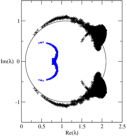
Figure 1: We compare the eigenvalue spectrum of $D_{\textrm{\scriptsize CI}}$ (+) with that of the reduced operator $D_{\textrm{\scriptsize CI,r}}$ ($\times$) for a typical configuration ($4^{4}$ lattice, $\beta_{1}=7.4$, $m_{\textrm{\scriptsize sea}}=0.1$); the latter are much closer to the value 1.

The accept/reject step involves the ratio of determinants of the Dirac operator. This is approximated by the stochastic estimator method inherent in the pseudo-fermion formulation. It was pointed out [18, 19, 20] that the noise in this stochastic estimation may introduce artificial barriers on the way through configuration space. Various methods to reduce the fluctuation of this estimate have been discussed. Following these ideas we introduced an additional UV-filter [21]. The basic concept is to reduce the spread of the eigenvalues of the operator to be stochastically estimated. One defines a reduced matrix

$$D_{\textrm{\scriptsize r}}=D\,\exp{(f(D))}\;,$$ (12)

where $f(D)$ is chosen to be a polynomial in $D$ with coefficients such that the eigenvalues of $D_{\textrm{\scriptsize r}}$ are concentrated around $z=1$ in the complex plane. In our acceptance step we need to compute

$$\frac{{\det}(D^{{\dagger}}\,D)_{\textrm{\scriptsize new}}}{{\det}(D^{{\dagger}}\,D)_{\textrm{\scriptsize old}}}=\exp{\left(-2\,\textrm{tr}\,f(D)_{\textrm{\scriptsize new}}+2\,\textrm{tr}\,f(D)_{\textrm{\scriptsize old}}\right)}\,\frac{{\det}(D_{\textrm{\scriptsize r}}^{{\dagger}}\,D_{\textrm{\scriptsize r}})_{\textrm{\scriptsize new}}}{{\det}(D_{\textrm{\scriptsize r}}^{{\dagger}}\,D_{\textrm{\scriptsize r}})_{\textrm{\scriptsize old}}}.$$ (13)

A complication for extended Dirac operators is to compute the trace over polynomials of $D$. However for $D_{\textrm{\scriptsize CI}}$ it is relatively straightforward to compute at least $\textrm{tr}(D)$ and $\textrm{tr}(D^{\dagger}D)$ . We tried a polynomial

$$f(D)=\gamma\,\textrm{tr}(D)+\delta\,\textrm{tr}(D^{\dagger}D)\;,$$ (14)

but found that introducing $\delta$ did not affect our results significantly. We therefore made the simplest choice $f(D)=\gamma\,D$ with $\gamma=-0.477$. In Fig. 1 we compare the eigenvalue spectrum of ${D_{\textrm{\scriptsize CI}}}$ with that of the reduced operator and find, indeed, that the reduced operator is closer to unity.

Our finally chosen updating method thus used this UV-filter combined with HYP-smearing and molecular dynamics equations using only the LW gauge action. Our trajectory lengths are 0.07 units of molecular dynamics time. In the actual implementation our trajectory consisted of a half step, a full step and a final half step in terms of the gauge field.

The acceptance itself is done in two steps. In the first step the value $\exp\left(-2\,\gamma\,\textrm{tr}\left(D_{\textrm{\scriptsize new}}-D_{\textrm{\scriptsize old}}\right)\right)$ is calculated exactly along with the change in the kinetic energy and bosonic part of the action. If this is accepted, the second – more expensive – step is the stochastic estimation of the ratio of determinants of the reduced matrices. The acceptance in the first step is $\sim 23\%$ and that of the second step is $\sim 20\%$. Although this gives an overall acceptance rate of less than $5\%$, one has to keep in mind that neither the first step nor the proposal involve any inversion of the fermion matrix and both are therefore quite fast. The only time consuming step is the second. Thus the net efficiency is to be compared with an HMC close to $\sim 20\%$ acceptance rate, albeit with smaller trajectory length.

Since the inversion of the chirally improved operator is the most expensive step in our algorithm we tried to increase its efficiency as much as possible. It is well-known [17] that during the trajectory development in standard HMC the inversion of the Dirac operator can be speeded up by using the solution vector of the previous step as the initial guess for the current step. Our case is slightly different. We do not invert the Dirac operator during our trajectory development, but our trajectory lengths are smaller. Therefore we expect that the new gauge field configuration $U_{\textrm{\scriptsize new}}$ is not too far away from the starting field configuration $U_{\textrm{\scriptsize old}}$. Also we note that the pseudo-fermion field $\phi$ is generated by $\phi={D_{\textrm{\scriptsize CI}}}(U_{\textrm{\scriptsize old}})\,\xi$, where $\xi$ is a complex gaussian random vector. Thus we have $\xi={D_{\textrm{\scriptsize CI}}}(U_{\textrm{\scriptsize old}})^{-1}\,\phi$ and we use this vector $\xi$ as an initial guess for the inversion. Indeed this choice reduces the necessary number of matrix-vector multiplications by about 20%.

Another speeding-up technique we use is to utilize the fact that we do not need to estimate the determinant ratio exactly. If $\eta$ is the random number with which we want to compare the ratio, then we need to check only if $(-\log\eta)$ is larger than the change in action or not [19]. For the overlap operator this can be implemented as follows. The Metropolis accept/reject step compares the norm of solution vector $x={D_{\textrm{\scriptsize Ov}}}^{-1}\,\phi$ with $(-\log\eta)$. At the $n$-th step of the bi-conjugate gradient routine, let the solution vector be $x_{n}$ and the residual vector $r_{n}=\phi-{D_{\textrm{\scriptsize Ov}}}\,x_{n}$. For the overlap operator one knows that

$$\frac{1}{2+m}|\phi|\leq|{D_{\textrm{\scriptsize Ov}}}^{-1}\phi|\leq\frac{1}{m}|\phi|\;.$$ (15)

Then it is straightforward to show that

$$|x_{n}|^{2}-\frac{2}{m}|x_{n}||r_{n}|+\frac{1}{(2+m)^{2}}|r_{n}|^{2}\leq|x|^{2}\leq|x_{n}|^{2}+\frac{2}{m}|x_{n}||r_{n}|+\frac{1}{m^{2}}|r_{n}|^{2}\;.$$ (16)

Since $D_{\textrm{\scriptsize CI}}$ satisfies the GW-relation (with $R=1/2$) to a good approximation, we assumed (and checked numerically) that its spectrum satisfies these bounds too. So at every step we only need to compute the upper and lower bounds on $|x|^{2}$ to see if $(-\log\eta)$ is inside that range or not. This reduces the number of matrix vector multiplications typically by a factor 3. For a test of our assumptions we check the accuracy of this method by computing the solution vector to an accuracy of $10^{-12}$ randomly once in 20 updates on the average. These tests never failed in our study.

We checked our numerics in several ways. Internal consistency of the program was checked by verifying the reversibility of the molecular dynamics trajectories. After a forward and backward trajectory the final energy was equal to the starting energy up to the precision of our calculations (double precision). As another check of the possible problem of using a noisy estimator we compared the stochastic estimator for the ratio of determinant with an exact evaluation (on the $4^{4}$ lattices). We found that the resulting plaquette expectation value was equal within errors (less than 0.15%) whether we calculated the determinant exactly or estimated it using the pseudo-fermions.

Further checks, also on $4^{4}$ lattices, were to reproduce the quenched plaquette values by turning off the fermions, reproduce dynamical Wilson results by replacing the chirally improved operator by the Wilson Dirac operator in the accept/reject step and reducing the chirally improved operator to the Wilson Dirac operator by changing the coefficients.

We have discussed in the introduction that the $D_{\textrm{\scriptsize CI}}$ parameters depend on the normalization parameter $z_{s}$ which is adjusted such that the massless operator has eigenvalues running through zero. This parameter is a function of $\beta_{1}$ and $m$. Also the LW-action parameters $\beta_{2}$ and $\beta_{3}$ are functions of $\beta_{1}$ and $m$. All of them, $z_{s}(\beta_{1},\,m)$, $\beta_{2}(\beta_{1},\,m)$ and $\beta_{3}(\beta_{1},\,m)$ have to be determined self-consistently by iterating the defining equations for $D_{\textrm{\scriptsize CI}}$ and the LW-action.

To determine $\beta_{2}$ and $\beta_{3}$ self-consistently due to (5) we used a “moving average” of the plaquette, i.e., the average of the plaquette over a reasonably large interval of successive updates, and set it to $u_{0}^{4}$. The interval is shifted with new updates by dropping the oldest point and adding a new one. The moving average has less fluctuations compared to the original plaquette and in equilibrium it is practically identical to the plaquette average. Once equilibrium is reached we do not change the gauge couplings any more. The final numbers are given in Table 1.

3 Results

In the quenched case for the LW-action the lattice spacing values for various values of $\beta_{1}$ have been determined in [22, 23]. For $\beta_{1}=7.6$ we have a lattice spacing $a\approx 0.19(1)$ fm, corresponding to a lattice size of 1.5 fm for the $8^{4}$ lattices in the quenched case.

Our final results are mainly from a simulation of the chirally improved Dirac operator on a $8^{4}$ lattice with the tadpole improved Lüscher-Weisz gauge action at $\beta_{1}=7.6$ and quark mass parameter $m_{\textrm{\scriptsize sea}}=0.1$. The measured plaquette value for this run (cf. Table 1) compares very well with the assumed plaquette value used for the determination of the LW-action (4). Unless explicitly stated otherwise, all results refer to this run; it is a sequence of 120000 updates. With our average acceptance rate of $\sim 5\%$ per update (i.e. per accept/reject step) and individual trajectory lengths of 0.07 this corresponds to a total effective molecular dynamics time of 420, counting only accepted steps. We allowed 40000 updates for equilibration and then saved a configuration every 2000 updates. All our propagators and masses have been computed on 40 such configurations. In computing the propagators an additional complication, compared to the quenched case, is that the masses of the sea-quarks and the valence-quarks should agree; one therefore cannot use multi-mass solvers.

The total run time for equilibration and configuration generation was about 2 weeks on a Linux cluster using 32 2.4 GHz Xeon CPU’s.

3.1 Equilibration

Equilibration for the chirally improved operator is a rather slow process. Also on a $4^{4}$ lattice we noticed that the number of matrix vector multiplications required were very high during the initial part of the cold start. This made cold starts quite impracticable for larger lattices. On the $8^{4}$ lattice we chose for our starting configurations quenched configurations with plaquette values significantly higher and lower than the expected dynamical equilibrium value and let the two sequences converge. The plaquette history for such a process is shown in Fig. 2, where we denote the plaquette value by $P=\frac{1}{3}\,\textrm{Re \,$\textrm{tr}$}\langle U_{\textrm{\scriptsize plaq}}\rangle$.

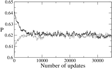
Figure 2: Equilibration of the plaquette for lattice size $8^{4}$, $\beta_{1}=7.6$ and quark mass $m_{\textrm{sea}}=0.1$.

Another important question is that of autocorrelation. Experience with exact HMC shows that very small step sizes lead to rather large autocorrelation times. We believe that with our trajectory length of $\Delta t=0.07$, the autocorrelation times are moderate. This is based on a quenched study of the autocorrelation time of the plaquette and we show the results in Fig. 3.

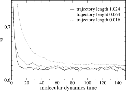
Figure 3: Equilibration of the plaquette from cold start as discussed in the text. The three different curves correspond to trajectory lengths of 1.024, 0.064 and 0.016 in molecular dynamics time.

From this figure we see that while the run with the trajectory length of 1.024 falls fastest, the run with trajectory length 0.064 is not too different from it after 20 time units whereas the run with length 0.016 is still quite far away. Assuming that such a picture also holds for the dynamical case, we conclude that our autocorrelation length is only moderately larger than for standard HMC where one typically uses a trajectory length $\sim 1$.

To get an idea of the autocorrelation time in our runs, we did a binned error analysis for the plaquette. We plot the result in Fig. 4. As can be seen clearly from the figure, the maximal error is obtained around a bin size of 2000, corresponding to an effective molecular dynamics time interval of 7. We take this to be an estimate of our autocorrelation time.

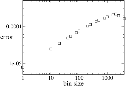
Figure 4: Variation of the error for the plaquette with bin size allowing for an estimate of the autocorrelation time ($8^{4}$ lattice, $\beta_{1}=7.6$ for the Lüscher-Weisz gauge action.)

Table 1: Measured plaquette values for different masses; $u_{0}^{4}$ denotes the assumed plaquette value.

$V$	$\beta_{1}$	$m_{\textrm{\scriptsize sea}}$	0.1	0.5	2.0	10.0	$\infty$
$4^{4}$	$7.4$	$U_{\textrm{\scriptsize plaq}}$	0.608(1)	0.604(1)	0.591(1)	0.579(1)	0.556(2)
		$u_{0}^{4}$	0.606	0.601	0.591	0.582	0.556
$8^{4}$	$7.6$	$U_{\textrm{\scriptsize plaq}}$	0.6202(2)				0.5824(1)
		$u_{0}^{4}$	0.62				0.5825

On a $4^{4}$ lattice we also studied the dependence of the plaquette expectation value on the quark mass. These studies were carried out for the Lüscher-Weisz action at $\beta_{1}=7.4$. The results are given in Table 1 together with the values for the simulation on the $8^{4}$-lattice. Since switching on dynamical fermions should in leading order be equivalent to going to larger $\beta_{1}$ in a quenched simulation, one expects that the plaquette value increases for decreasing sea-quark mass. This is indeed what we observe.

3.2 Spectrum of the Dirac operator

The chirally improved Dirac operator is an approximate solution of the Ginsparg-Wilson relation. In particular it has the property that the low lying spectrum is close to the Ginsparg-Wilson circle. In order to verify that this property was preserved also with dynamical quarks, we plot the first 100 eigenvalues for three equilibrium configurations in Fig. 5, comparing the quenched with the dynamical situation. Compared to the quenched case the spectrum in the dynamical case is closer to the circle, indicating smaller effective lattice spacing.

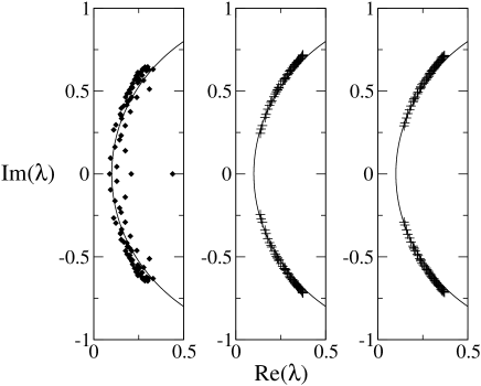
Figure 5: Spectra of the chirally improved operator on a $8^{4}$ lattice. $\beta_{1}$ for the Lüscher-Weisz gauge action was 7.6 and the quark mass $m=0.1$. These spectra are for three typical, randomly selected quenched (diamonds) and dynamical (plus) configurations.

Zero modes of the Dirac operator are related to instantons. For the chirally improved operator, in the quenched as well as the dynamical case with large quark masses, zero modes are observed. However for the mass 0.1 of our $8^{4}$ simulation we did not find any zero modes after equilibration.

In order to understand this feature, which seems to contradict other findings [5, 6] we also ran simulations with the Wilson Dirac operator on a $4^{4}$ lattice. Here we did see would-be zero modes (i.e. reasonably small real eigenvalues) quite frequently. This may be due to the fact that the fluctuations of the Wilson Dirac operator seem to be much larger than the chirally improved operator. In fact with our algorithm we were not able to simulate the Wilson Dirac operator on the larger $8^{4}$ lattice. The fluctuations of the fermionic determinant were far too large for any reasonable trajectory length.

As a further check we also replaced the stochastic estimator for the determinant by the exact evaluation for the small lattice runs. The tunneling behavior did not change. Even when we started with a topologically non-trivial quenched configuration (i.e., zero modes of $D_{\textrm{\scriptsize CI}}$ for the quenched gauge configuration) the configurations quickly tunneled to the zero-topological charge sector while performing the HMC updates. We conclude that there is no obvious tunneling barrier in our algorithm but that the trivial zero mode sector is natural for our choice of couplings.

Recent results on the dynamical overlap fermions do report seeing zero modes [5, 6]. However, the plaquette values quoted in [5] are quite different from ours; indications are that those runs are effectively at smaller $\beta$ than ours. That coupling leads to a larger physical volume (and lower temperature) and it is not obvious that the results can be compared. The results of [6] extend to similar parameter values as ours and tunneling to sectors with one zero mode were observed. We work at a slightly larger gauge coupling, and, as argued below, we may be deeper in the deconfined phase. More statistics and fine tuning of the parameters will be necessary to resolve this discrepancy.

3.3 Propagators

One of the primary goals of lattice simulations is to reproduce the known hadron mass spectrum. Although the lattice size is definitely too small to identify asymptotic states, we still have computed pion and rho meson propagators with our dynamical chirally improved configurations for a crude, preliminary check. The propagators were computed using point sources and sinks. Our expressions for the pion and the rho correlators are given by

$$C_{\pi}(0,t) = \sum_{\vec{x}}\textrm{tr}\left(\gamma_{5}\,{D_{\textrm{\scriptsize CI}}}^{-1}(\vec{x},t:0,0)\,\gamma_{5}\,{D_{\textrm{\scriptsize CI}}}^{-1}(0,0:\vec{x},t)\right)\;,$$ (17)

$$C_{\rho}(0,t) = \sum_{\vec{x},i=1,2,3}\textrm{tr}\left(\gamma_{i}\,{D_{\textrm{\scriptsize CI}}}^{-1}(\vec{x},t:0,0)\,\gamma_{i}\,{D_{\textrm{\scriptsize CI}}}^{-1}(0,0:\vec{x},t)\right)\;.$$ (18)

The correlation functions are shown in Fig. 6 for the dynamical ($m_{\textrm{\scriptsize sea}}=m_{\textrm{\scriptsize val}}=0.1$) as well as for the quenched ($m_{\textrm{\scriptsize val}}=0.1$) case. The error bars are naively determined without auto-correlation analysis.

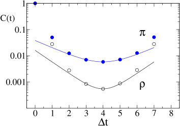
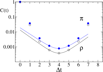
Figure 6: Normalized pion (full circles) and rho (open circles) correlators on a $8^{4}$ lattice. We compare the quenched results (left-hand plot) with the dynamical ones (at $m_{\textrm{\scriptsize sea}}=0.1$, right-hand plot), both at $\beta_{1}=7.6$ and valence-quark mass $m_{\textrm{\scriptsize val}}=0.1$. The curves represent the $\cosh$-fits to the three central points.

Table 2: Fitted mass values in lattice units for lattice size $8^{4}$, $\beta_{1}=7.6$ and valence-quark mass $m_{\textrm{\scriptsize val}}=0.1$.

		Pion		Rho
simulation	range of $\Delta\,t$	$m_{\pi}$	$\chi^{2}/d.o.f$	$m_{\rho}$	$\chi^{2}/d.o.f$
dynamical	2$-$6	1.18 (3)	10.54	1.33 (4)	10.62
	3$-$5	0.97 (1)	0.02	1.06 (2)	0.14
quenched	2$-$6	0.71 (1)	0.13	1.21 (4)	8.16
	3$-$5	0.64 (2)	0.03	1.02 (6)	1.62

Some conclusions can be drawn comparing the propagators of the dynamical with those of the quenched case. Table 2 shows the results for the “meson masses” $m$ of our $\cosh(m\,(t-n_{T}/2))$-fits in the symmetry region. Let us denote the dimensionless masses by $m^{q}$ (for quenched) and $m^{d}$ (for dynamical) and use the values from the smaller fit range (with better $\chi^{2}/d.o.f$). We find $m_{\pi}^{d}/m_{\pi}^{q}\approx 1.52$ and $m_{\rho}^{d}/m_{\rho}^{q}\approx 1.04$. There can be two reasons for this. Either the lattice spacing has increased in the dynamical case or it has decreased so much that we are at much smaller physical time extent and therefore cannot observe the asymptotic decay of the correlators. Our spectrum, as discussed in the previous section, suggests that the second explanation is more plausible. Thus we cannot use these values to derive the lattice spacing.

On the other hand, comparing the ratio of the fitted “masses” $m_{\pi}/m_{\rho}$ for the dynamical and the quenched cases (0.92 vs. 0.63) we see that the dynamical ratio is much higher. In the quenched case such a behavior is observed for increased valence-quark masses. Since the dimensionless valence-quark mass had the same value 0.1 in both cases we can use the meson mass ratio to try to obtain an effective quenched $\beta_{1}$ (or lattice spacing) for our dynamical simulation. Results from the BGR-collaboration’s [11] quenched studies at values up to $\beta_{1}=8.7$ (lattice spacing 0.078 fm) leads us to crudely estimate the gauge coupling to lie beyond 8.7, corresponding to a lattice spacing $a\lesssim 0.08$ fm.

3.4 Polyakov loop

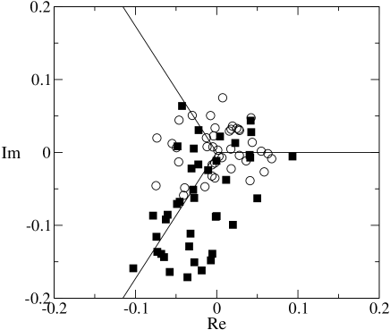
Figure 7: Scatter plot of the Polyakov loop for the quenched (open symbols) and the dynamical (full symbols, $m_{\textrm{\scriptsize sea}}=0.1$) situation for lattice size $8^{4}$ and $\beta_{1}=7.6$.

For dynamical quarks the Polyakov-loop is not an order parameter and for intermediate values of the dynamical quark mass there may be no phase transition at all but just a crossover region, analytically connecting the confinement region with the plasma phase. Nevertheless, the Polyakov-loop is at least an indicator for the location of that crossover region. In Fig. 7 we compare the values obtained for the quenched and the dynamical case. We find that the center symmetry of the confinement phase is broken for the dynamical situation. This confirms our argument that the effective lattice spacing has decreased considerably.

Since we are working on a symmetric lattice of size $8^{4}$ we are not really entitled to call $T=1/(8\,a)$ a temperature in a strict sense. However, assuming a transition temperature range of $T_{c}\approx$ 250 MeV (quenched calculations give $T_{c}\approx$ 270 MeV, dynamical simulations at smaller quark mass give $T_{c}\approx$ 170-190 MeV [24]) and still comparing it with $T$ we find that $a\leq 0.1$ fm for our dynamical situation. This is significantly smaller than the quenched value $0.19(1)$ fm.

This explains the missing zero modes. The dynamical system is too small to accommodate instantons and is already in the plasma-like regime.

4 Conclusions

We conclude that introducing dynamical fermions for chirally improved fermions is possible with reasonable effort. HMC in the simplified version appears to work, and dynamical fermions, although still with relatively large mass, make a difference in the results as compared to the quenched case.

For the gauge coupling used we find evidence that the effective lattice spacing decreases considerably when switching on dynamical fermions. Although with our data we cannot derive values for the lattice spacing we have several observations indicating the drastic decrease:

• The Dirac operator spectrum becomes smoother and closer to the GW-circle. Tunneling from non-trivial topological sectors to the trivial one is observed, but the system then stays in the sector without zero modes.

• The mass ratio of pion over rho as derived approximately from the correlation functions becomes larger. Since the dimensionless valence-quark mass is kept constant this corresponds to a larger physical valence-quark mass but smaller lattice spacing, similar to the observations in the quenched system.

• The Polaykov loop shows breaking of the center symmetry.

All these effects are observed when increasing $\beta_{1}$ in a quenched simulations. Curves of constant physics in the $(\beta_{1},m_{\textrm{\scriptsize sea}})$ plane bend towards smaller gauge coupling for decreasing $m_{\textrm{\scriptsize sea}}$. We estimate that the effective lattice spacing has changed from 0.19 fm for the quenched simulation at $\beta_{1}=7.6$ to a value below 0.1 fm for $m_{\textrm{\scriptsize sea}}=0.1$.

Obviously we should work on lattices with larger time extension for better analysis of the propagators and at smaller $\beta_{1}$ as a next step. Also desirable is an estimate of the growth of the computational effort with decreasing sea-quark mass. In view of our results and within these caveats we can be optimistic to apply the chiral improved fermion action to a realistic simulation of QCD.

Acknowledgment: We wish to thank Christof Gattringer for helpful comments; we are also grateful to Nigel Cundy, Stefan Schaefer and Peter Weisz for discussions. Support by Fonds zur Förderung der Wissenschaftlichen Forschung in Österreich, projects M767-N08 (Lise-Meitner Fellowship) and P16310-N08 is gratefully acknowledged.

References

- [1] P. H. Ginsparg and K. G. Wilson, Phys. Rev. D 25 (1982) 2649.
- [2] A. Bode, U. M. Heller, R. G. Edwards, and R. Narayanan, hep-lat/9912043 (1999).
- [3] Z. Fodor, S. D. Katz, and K. K. Szabo, JHEP 0408 (2004) 003; and hep-lat/0409070 (2004).
- [4] N. Cundy, A. Frommer, J. van der Eshof, S. Krieg, and K. Schäfer, hep-lat/0405003 (2004).
- [5] N. Cundy, S. Krieg, A. Frommer, T. Lippert, and K. Schilling, hep-lat/0409029 (2004).
- [6] T. DeGrand and S. Schaefer, hep-lat/0412005 (2004).
- [7] R. Narayanan and H. Neuberger, Phys. Lett. B 302 (1993) 62; Nucl. Phys. B 443 (1995) 305.
- [8] D. B. Kaplan, Phys. Lett. B 288 (1992) 342. V. Furman and Y. Shamir, Nucl. Phys. B 439 (1995) 54.
- [9] P. Hasenfratz and F. Niedermayer, Nucl. Phys. B 414 (1994) 785.
- [10] C. Gattringer, Phys. Rev. D 63 (2001) 114501. C. Gattringer, I. Hip, and C. B. Lang, Nucl. Phys. B 597 (2001) 451.
- [11] C. Gattringer et al., Nucl. Phys. B 677 (2004) 3.
- [12] T. Burch et al., Phys. Rev. D 70 (2004) 054502.
- [13] http://physik.uni-graz.at/ cbl/research/data/dci/, 2003.
- [14] A. Hasenfratz and F. Knechtli, Phys. Rev. D 64 (2001) 034504.
- [15] M. Alford, W. Dimm, G. P. Lepage, G. Hockney, and P. B.Mackenzie, Phys. Lett. B 361 (1995) 87.
- [16] D. H. Weingarten and D. N. Petcher, Phys. Lett. B 99 (1981) 333.
- [17] S. Gottlieb, W. Liu, D. Toussaint, R. L. Renken, and R. L. Sugar, Phys. Rev. D 35 (1986) 2531. S. Duane, A. D. Kennedy, B. J. Pendleton, and D. Roweth, Phys. Lett. B 195 (1987) 216.
- [18] M. Hasenbusch, Phys. Rev. D 59 (1999) 054505.
- [19] A. Alexandru and A. Hasenfratz, Phys.Rev. D 66 (2002) 094502.
- [20] M. A. Clark and A. D. Kennedy, hep-lat/0409134 (2004).
- [21] P. de Forcrand, Nucl. Phys. B (Proc. Suppl.) 73 (1999) 822.
- [22] C. Gattringer, R. Hoffmann, and S. Schaefer, Phys. Rev. D 65 (2002) 094503.
- [23] M. Alford, W. Dimm, G. P. Lepage, G. Hockney, and P. B. Mackenzie, Nucl. Phys. B (Proc. Suppl.) 42 (1995) 787.
- [24] F. Karsch, Nucl. Phys. B (Proc. Suppl.) 83-84 (2000) 14.