MPP-2004-152

December 2004

The $4d$ one component lattice $\phi^{4}$ model in the broken phase revisited

Janos Balog

Research Institute for Particle and Nuclear Physics

1525 Budapest 114, Pf. 49, Hungary

Anthony Duncan, Ray Willey

Department of Physics, 100 Allen Hall

University of Pittsburgh, Pittsburgh, PA 15260, USA

Ferenc Niedermayer^∗

Institute for Theoretical Physics, University of Bern

CH-3012 Bern, Switzerland

Peter Weisz

Max-Planck-Institut für Physik

Föhringer Ring 6, D-80805 München, Germany

Abstract

Measurements of various physical quantities in the symmetry broken phase of the one component lattice $\phi^{4}_{4}$ with standard action, are shown to be consistent with the critical behavior obtained by renormalization group analyses. This is in contrast to recent conclusions by another group, who further claim that the unconventional scaling behavior they observe, when extended to the complete Higgs sector of the Standard Model, would alter the conventional triviality bound on the mass of the Higgs.

—————
^∗On leave from Eötvös University, HAS Research Group, Budapest, Hungary

1 Introduction

The continuum limit of the lattice regularized $\phi^{4}$ theory in 4 dimensions with $n\geq 1$ components is thought to be trivial. The evidence comes from renormalization group studies and numerical simulations; remarkably however there is still no rigorous proof.

After a period of intense numerical investigations about 15 years ago, interest in this model within the lattice community dwindled. Occasionally however some authors have questioned the usual procedures of renormalization in the broken phase. In their latest paper [?] Cea, Consoli and Cosmai claim to present further numerical evidence for their scenario. From the presentation of the results in their paper a neutral reader would, accepting their analysis, indeed conclude that the conventional wisdom (CW) concerning the critical behavior in the lattice $\phi^{4}$ was incorrect. The purpose of this paper is to point out the deficiencies of their analyses, and to show that the numerical data is completely consistent with the conventional picture.

2 The lattice theory and renormalization group predictions

The standard lattice $\phi^{4}$ model is characterized by two bare parameters $\kappa,\lambda$; the action is

$$S=\sum_{x}\left[-2\kappa\sum_{\mu=1}^{4}\phi(x)\phi(x+\hat{\mu})+\phi(x)^{2}+\lambda(\phi(x)^{2}-1)^{2}\right]\,.$$ (2.1)

There are two phases separated by a line of critical points $\kappa=\kappa_{\rm c}(\lambda)$. For $\kappa>\kappa_{\rm c}(\lambda)$ the symmetry is spontaneously broken and the bare field $\phi(x)$ has a non-vanishing expectation value $v$. As usual this is defined by first taking the thermodynamic limit in the presence of an external uniform magnetic field $h$ and then letting this field tend to zero

$$v=\lim_{h\to 0}\lim_{V\to\infty}\langle\phi(0)\rangle_{h}\,.$$ (2.2)

This study will restrict attention to the vacuum expectation value and the connected two-point function

$$G(x)=\langle\phi(x)\phi(0)\rangle_{\rm c}=\langle\phi(x)\phi(0)\rangle-v^{2}\,.$$ (2.3)

A renormalized mass $m_{{\hbox{\sixrm R}}}$ and a field wave function renormalization constant $Z_{{\hbox{\sixrm R}}}$ are defined through the behavior of Fourier transform of $G(x)$ for small momenta:

$$\tilde{G}(k)^{-1}=Z_{{\hbox{\sixrm R}}}^{-1}\left\{m_{{\hbox{\sixrm R}}}^{2}+k^{2}+{\rm O}(k^{4})\right\}\,.$$ (2.4)

The susceptibility $\chi$ and the second moment $\mu$ are defined through

$$\chi = \sum_{x}G(x)=Z_{{\hbox{\sixrm R}}}/m_{{\hbox{\sixrm R}}}^{2}\,,$$ (2.5)

$$\mu = \sum_{x}\,x^{2}G(x)=8Z_{{\hbox{\sixrm R}}}/m_{{\hbox{\sixrm R}}}^{4}\,.$$ (2.6)

We also define the normalization constant associated with the canonical bare field through

$$\widehat{Z_{{\hbox{\sixrm R}}}}=2\kappa Z_{{\hbox{\sixrm R}}}=2\kappa m_{{\hbox{\sixrm R}}}^{2}\chi\,.$$ (2.7)

In the framework of perturbation theory correlation functions of the multiplicatively renormalized field

$$\phi_{{\hbox{\sixrm R}}}(x)=Z_{{\hbox{\sixrm R}}}^{-1/2}\phi(x)\,,$$ (2.8)

have at all orders finite continuum limits after mass and coupling renormalization are taken into account. Correspondingly a renormalized vacuum expectation value is defined through

$$v_{{\hbox{\sixrm R}}}=vZ_{{\hbox{\sixrm R}}}^{-1/2}\,.$$ (2.9)

Here we adopt the generally accepted assumption that the structurally same multiplicative renormalization is required to define the continuum limit of the theory non-perturbatively. We see no evidence for the claim in ref. [?] that the vacuum expectation value and the fluctuating part of the bare field should be renormalized differently. Finally a particular renormalized coupling is defined by

$$g_{{\hbox{\sixrm R}}}\equiv 3m_{{\hbox{\sixrm R}}}^{2}/v_{{\hbox{\sixrm R}}}^{2}=3m_{{\hbox{\sixrm R}}}^{4}\chi/v^{2}\,,$$ (2.10)

as is one popular choice in the perturbative framework.

The commonly accepted picture of the critical behavior of the theory is mainly due to the work of the Saclay group [?]. In their framework the renormalization group equations predict that the mass and vacuum expectation value go to zero according to

$$m_{{\hbox{\sixrm R}}} \propto \tau^{1/2}|\ln(\tau)|^{-1/6}\,,$$ (2.11)

$$v_{{\hbox{\sixrm R}}} \propto \tau^{1/2}|\ln(\tau)|^{1/3}\,,$$ (2.12)

for $\tau=\kappa/\kappa_{\rm c}-1\to 0$, and correspondingly the renormalized coupling is predicted to go to zero logarithmically which is the expression of triviality. The critical behavior in the broken phase is conveniently expressed in terms of three integration constants $C^{\prime}_{i}\,,i=1,2,3$ appearing in the critical behaviors:

$$m_{{\hbox{\sixrm R}}} = C^{\prime}_{1}(\beta_{1}g_{{\hbox{\sixrm R}}})^{17/27}{\rm e}^{-1/\beta_{1}g_{{\hbox{\sixrm R}}}}\left\{1+{\rm O}(g_{{\hbox{\sixrm R}}})\right\}\,,\,\,\,\,\beta_{1}=\frac{3}{16\pi^{2}}\,,$$ (2.13)

$$Z_{{\hbox{\sixrm R}}} = C^{\prime}_{2}\left\{1-\frac{7}{36}\frac{g_{{\hbox{\sixrm R}}}}{16\pi^{2}}+{\rm O}(g_{{\hbox{\sixrm R}}}^{2})\right\}\,,$$ (2.14)

$$\kappa-\kappa_{\rm c} = \frac{1}{2}C^{\prime}_{3}m_{{\hbox{\sixrm R}}}^{2}g_{{\hbox{\sixrm R}}}^{-1/3}\left\{1+{\rm O}(g_{{\hbox{\sixrm R}}})\right\}\,.$$ (2.15)

In ref. [?] these constants were estimated by relating them to the corresponding constants $C_{i}$ in the symmetric phase. These in turn were computed by integrating the renormalization group equations with initial data on the line $\kappa=0.95\kappa_{\rm c}(\lambda)$ obtained from high temperature expansions.

3 Some proposed criticisms of CW

In ref. [?] the authors present two quantitative arguments against the conventional wisdom. Their work considers just the Ising limit ($\lambda=\infty$). Firstly they claim $Z_{{\hbox{\sixrm R}}}$ grows logarithmically as one approaches the critical point instead of going to a constant as predicted by the RG (see Eq. (2.14)). Unfortunately they only measure $v,\chi$ which is not sufficient to determine $Z_{{\hbox{\sixrm R}}}$. To overcome this deficiency they compute $\widetilde{Z_{{\hbox{\sixrm R}}}}=m_{\rm input}^{2}\chi$, where $\chi$ is their MC measurement at a given value of $\kappa$ but $m_{\rm input}$ is an estimate of $m_{{\hbox{\sixrm R}}}$ at the same $\kappa$ taken from Table 3 of ref. [?] (referred to as T3 below). This “composed” quantity $\widetilde{Z_{{\hbox{\sixrm R}}}}$ indeed seems to grow as the critical point is approached. Accepting that their measurements of $\chi$ are correct (and indeed we agree with their values on the lattices we checked), the crucial question is whether the estimates $m_{\rm input}$ of $m_{{\hbox{\sixrm R}}}$ are reliable.

At this stage two details of the analysis in ref. [?] must be appreciated. Firstly the values of $\kappa$ cited in the last column of T3 are written using $\kappa_{\rm c}$ obtained from the same procedure of analysis for all values of $\lambda$ . For the particular case of the Ising model there are (presumingly) more accurate values; some comparisons are made in Table 1. Hence, even if one accepts the estimated errors in T3, estimates of $m_{{\hbox{\sixrm R}}}$ for a given $\kappa$ obtained using this table naively are subject to further large uncertainties.

$\,\,\,\,\,\,\,\kappa_{\rm c}$	ref.
$0.07475(7)$	[?]
$0.074834(15)$	[?]
$0.074848(2)$	[?]
$0.074851(8)$	[?]
$0.07487(5)$	[?]

Table 1: Estimates of $\kappa_{\rm c}$ in the 4$d$ Ising model.

Secondly it is probable that the systematic errors in T3 have been underestimated. This stems from a probable underestimate on the size of the systematic errors on the cited values of the integration constants $C^{\prime}_{i}$; e.g. the estimated values of the constants obtained by using 2-loop or 3-loop expressions in the RG equations differ considerably. This question was briefly addressed in the 3rd paragraph sect. 5.2 of [?] and later stressed by Peter Hasenfratz [?] .

The simple outcome of the discussion above is that to compute $Z_{{\hbox{\sixrm R}}}$ and $m_{{\hbox{\sixrm R}}}$ independently one needs accurate measurements of both $\chi,\mu$. In the next sections we describe such measurements and find that the computed values of $Z_{{\hbox{\sixrm R}}}$ are consistent with the RG expectation in the $\phi^{4}$ theory. For the Ising limit the measured values of $m_{{\hbox{\sixrm R}}}$ are considerably lower than the corresponding estimates $m_{\rm input}$ in [?].

The second presented “evidence” against CW in [?] concerns the quantity $v^{2}\chi$. Defining

$${\ell}\equiv-\ln(\kappa-\kappa_{\rm c})\,,$$ (3.16)

in the RG framework $v^{2}\chi$ behaves as $\propto{\ell}$ as one approaches $\kappa_{\rm c}$, whereas in their scenario they expect a more singular behavior $\propto{\ell}^{2}$. Figure 2 in [?] gives the impression that the data strongly supports their prediction. However, this impression is completely false! The figure is obtained by 2-parameter fits of $v^{2}\chi$ with functions $A\ln^{p}(\kappa-\kappa_{\rm c})$ with $p=1,2$ and $\kappa_{\rm c}$ a fit parameter. But such fits are of course meaningless without including a scale of the logarithm. Once this is done (as described in subsect. 4.4), one gets a beautiful fit to the data also for the function expected from the RG group.

4 Ising MC simulation and results

In this section we present our simulations of the 4$d$ Ising model on a hypercubic lattice with periodic boundary conditions in all directions. We consider only geometries with volumes $V=L^{3}T$.

4.1 Simulation algorithm

For updating the configurations we used the Swendsen-Wang cluster method [?]. Beyond practically eliminating the problem of critical slowing down, the method allows to use improved estimators which reduce significantly the errors of the measured quantities. Since the application of the cluster improved estimators have some specific features for the broken phase, we discuss briefly here the applied procedure.

The first step in the SW cluster algorithm is to put bonds between neighboring spins of equal signs with probability $p=1-\exp(-4\kappa)$, while no bonds are put between spins with opposite signs. In the second step one identifies the clusters, the set of spins connected by bonds. Obviously, spins within a cluster have the same sign. Denote the number of clusters by $\nu$, and the number of sites in the $i$-th cluster by $n_{i}$, $i=1,\ldots,\nu$. Assume for convenience that the numbering is chosen so that $n_{1}\geq n_{2}\geq\ldots\geq n_{\nu}$. In the updating step one flips all spins in the $i$-th cluster with probability 1/2. All resulting $2^{\nu}$ configurations appear in the equilibrium distribution with equal probability. The cluster improved estimator replaces a quantity by its average over these $2^{\nu}$ configurations. In particular the product $\phi(x)\phi(y)$ is replaced by $+1$ if $x$ and $y$ belong to the same cluster, and by $0$ if the two sites belong to different clusters.

4.2 Determination of $v$ and $\chi$

The difference between the symmetric and broken phase shows up in the distribution of the cluster size. In the symmetric phase (at finite correlation length $\xi$) the typical size of clusters is determined by $\xi$ and remains finite and independent of $L$ for $L\gg\xi$. This is obvious from considering the spin-spin correlator $G(x)$ at large distances $|x|$ since this number is equal to the probability that the two sites are within the same cluster. As a consequence, this probability goes down exponentially with the distance. It is easy to show that in the symmetric phase the susceptibility is given by $\chi=\left\langle\frac{1}{V}\sum_{i}n_{i}^{2}\right\rangle\,.$

In the broken phase (in infinite volume) $\langle\phi(x)\phi(y)\rangle\to v^{2}$ for $|x-y|\to\infty$. This involves that the size of the largest cluster grows proportionally to the volume, $\langle n_{1}\rangle\propto V$ while the distribution of $n_{i}$, $i=2,3,\ldots$ is not affected by the volume for $L,T\gg\xi$ (and is characterized by the correlation length). In this case (for $V\to\infty$) the vacuum expectation value is given by

$$v=\frac{1}{V}\langle n_{1}\rangle\,,$$ (4.17)

and the susceptibility by

$$\chi=\left\langle\frac{1}{V}\sum_{i>1}n_{i}^{2}\right\rangle+\frac{1}{V}\left(\langle n_{1}^{2}\rangle-\langle n_{1}\rangle^{2}\right)\,.$$ (4.18)

In sufficiently large volumes the definition Eq. (4.17) of the vev coincides with the conventional definition Eq. (2.2). For sufficiently large $V$ in the broken phase one can choose an external field $h$ such that $h\langle n_{1}\rangle=hvV\gg 1$ and at the same time $hn_{2}\ll 1$. Therefore in the presence of the magnetic field the spins in the largest cluster are frozen to value $+1$ while $h$ has practically no influence on the orientation of the other clusters. Eq. (4.17) provides a convenient definition of $v$ in a finite volume. For large enough volumes this definition also coincides practically with the Binder’s definition [?] using the absolute value of the total magnetization:

$$v_{\rm Binder}=\left\langle\frac{1}{V}|\sum_{x}\phi(x)|\right\rangle\,,$$ (4.19)

which is the definition employed in ref. [?]. For a thorough discussion of various finite volume definitions of the vev (and more general finite volume effects in this model) we refer the reader to ref. [?]. Assigning random signs to the clusters $i=2,\ldots,\nu$ the sum of spins in these clusters has a variance $\sum_{i=2}^{\nu}n_{i}^{2}\lesssim V\chi$ (cf. Eq. (4.18)), while the value of the spin in the largest cluster is $n_{1}\sim vV$. The probability that the random component has the same magnitude as the constant component $n_{1}$ is suppressed at least by the factor $\exp(-Vv/\chi^{2})\,.$

Note that for the case of $V=L^{3}T$, $L=\mathrm{fixed}$, $T\to\infty$ the situation is somewhat different. In this quasi-one-dimensional case the large clusters have finite length in the $t$-direction, although much larger than $L$. Their typical length is given by the inverse of the energy gap between the lowest even and odd eigenstates of the transfer matrix [?]. Here we shall not discuss this geometry, note only the obvious fact that any quantity defined through spin correlators can be expressed in terms of expectation values of the cluster sizes $n_{i}$.

Apart from $v$ and $\chi$ we also measured the time-slice correlation functions

$$S(t)=\sum_{{\bf x}}G((t,{\bf x}))\,,$$ (4.20)

to compute the exponential mass and the Fourier transform $\tilde{G}(k)$ at momenta $k$ along the $t$-axis.

Typically we performed more than $400$K sweeps at each $\kappa$ point. The autocorrelation times for the vev and the two point function $S(t=T/4)$ were monitored and found reasonably small e.g. for the lattice with the largest correlation length which we measured ($\kappa=0.0751$) they were $\sim 8,\sim 3$ respectively.

4.3 Raw data and analysis

To illustrate the quality of the raw data, and for later reference, in Table 2 the time-slice correlation function $S(t)$ is given for $V=48^{4}$ at $\kappa=0.0751$.

$t$	$S(t)$	$t$	$S(t)$	$t$	$S(t)$	$t$	$S(t)$
0	17.788(31)	7	5.320(27)	14	1.666(25)	21	0.646(29)
1	14.913(31)	8	4.492(26)	15	1.421(25)	22	0.600(29)
2	12.529(30)	9	3.796(26)	16	1.217(26)	23	0.573(30)
3	10.540(30)	10	3.211(25)	17	1.048(26)	24	0.563(30)
4	8.875(29)	11	2.720(25)	18	0.909(27)
5	7.478(28)	12	2.306(25)	19	0.798(27)
6	6.306(28)	13	1.958(25)	20	0.711(28)

Table 2: The (subtracted) time-slice correlation function $S(t)$ for the Ising case at $\kappa=0.0751$ on a $48^{4}$ lattice. Note that the quoted errors for this quantity are much smaller than that for the subtracted term $v^{2}L^{3}=2711.1(1.2)$.

In Table 3 we collect data of the values of $v,\chi$ for various values of $\kappa,L$ from two papers [?,?] together with our own. The simulation at the largest value of $\kappa=\kappa_{0}$ was performed to test our programs and analyses by comparison at a point where the low temperature expansion is considered quantitatively reliable [?]. The agreement between the data and analytic computations is indeed satisfactory. As for the values of $\kappa$ closer to $\kappa_{\rm c}$, firstly one observes excellent agreement of the raw data on those lattices measured by different groups. Thus we are confident that the raw data (albeit sometimes obtained by different methods) can be trusted. Secondly at values of $\kappa$ where different volumes were measured there are no signs of significant finite volume effects.

$\,\,\,\,\,\kappa$	$L$	$\chi$	$\,\,\,\,\,\,\,\,v$	$\,\,\,v^{2}\chi$	ref.
$\kappa_{0}$	$10$	$5.130(2)$	$0.571267(8)$	$1.674(1)$
$0.077$	$16$	$18.18(2)$	$0.38947(2)$	$2.758(4)$	[?]
$0.076$	$20$	$37.85(6)$	$0.30158(2)$	$3.442(6)$	[?]
$0.076$	$20$	$37.80(6)$	$0.30151(3)$	$3.437(6)$
$0.076*$	$20$	$37.84(6)$	$0.30158(2)$	$3.442(6)$
$0.0759$	$32$	$41.71(13)$	$0.29030(2)$	$3.515(12)$	[?]
$0.0759$	$48$	$41.95(93)$	$0.29028(5)$	$3.535(79)$	[?]
$0.075628$	$48$	$58.70(42)$	$0.25580(2)$	$3.841(28)$	[?]
$0.0754$	$32$	$87.45(76)$	$0.22054(8)$	$4.253(40)$	[?]
$0.0754$	$32$	$86.95(55)$	$0.22055(6)$	$4.229(29)$
$0.0754$	$48$	$87.82(56)$	$0.22048(2)$	$4.269(28)$	[?]
$0.075313$	$48$	$104.2(1.3)$	$0.20477(4)$	$4.367(56)$	[?]
$0.075231$	$60$	$130.8(1.4)$	$0.18812(3)$	$4.629(50)$	[?]
$0.0752$	$36$	$142.1(8)$	$0.18138(5)$	$4.674(29)$
$0.0752$	$48$	$142.6(9)$	$0.18132(4)$	$4.689(32)$
$0.0751$	$48$	$203.8(3.1)$	$0.15665(10)$	$5.002(82)$	[?]
$0.0751$	$48$	$206.4(1.2)$	$0.15657(4)$	$5.060(32)$
$0.0751$	$52$	$201.2(6.2)$	$0.15654(7)$	$4.93(15)$	[?]
$0.0751$	$60$	$202.4(8.6)$	$0.15648(2)$	$4.96(21)$	[?]
$0.074968$	$68$	$460.2(4.9)$	$0.11261(5)$	$5.836(67)$	[?]
$0.0749$	$68$	$1125(36)$	$0.07736(12)$	$6.73(24)$	[?]
$0.0749$	$72$	$1141(39)$	$0.07752(21)$	$6.86(27)$	[?]

Table 3: Measured values of $\chi,v$ from various Ising simulations; data from this investigation have no entry in the last column. $\kappa_{0}=0.080795$. In all cases $T=L$ except for the lattice where $\kappa=0.076^{*}$ denotes $L=20,T=32$.

The second moment mass can be determined directly from the Fourier transform of $S(t)$ (i.e. $\tilde{G}(k)$ with momenta along the $t$-axis) using Eq. (2.4) which involves a determination of the slope from the available discrete values of $k$. To avoid possible discretization errors due to the finiteness of the lattice size $T$ we also used the following procedure to determine $m_{{\hbox{\sixrm R}}}$ and $Z_{{\hbox{\sixrm R}}}$. We first computed the exponential mass $m$ characterizing the exponential fall-off of the time-slice correlation functions at large separations, using one-mass and constrained two-mass fits (where the second mass was required to satisfy $m_{2}\gtrsim 2m$). For the one-mass fit we included only distances $t$ with $mt\gtrsim 1$. The results of the two fits were completely consistent, the central value of the 2-mass fit being slightly lower but the estimated errors larger than those of the 1-mass fit. In Table 4 we quote only the outcome of the 1-mass fit. Note that the value of $mL$ is in each case large $\gtrsim 8$, and hence finite volume effects are expected to be smaller than our statistical errors. An estimate of the infinite volume second moment mass was then computed from the sums $\sum_{t}S(t)$ and $\sum_{t}t^{2}S(t)$, where for $|t|<T_{0}$ (some large $T_{0}\leq T/2$) we took the measured correlations and for $T_{0}\leq|t|<\infty$ we estimated $S(t)$ by assuming it has the form of a free lattice correlator with the previously determined mass $m$ and amplitude. The resulting estimates of $m_{{\hbox{\sixrm R}}}$ from the two fits hardly differed; in Table 4 we quote the results from the 1-mass fit. The measurements of $m_{{\hbox{\sixrm R}}}$ from $\tilde{G}(k)^{-1}$ were also consistent with the values in the table (although statistical errors were typically a factor $\sim 2$ larger), again indicating small finite volume effects. We also remark that the relations between the quoted $m_{{\hbox{\sixrm R}}}$ and $m$ are consistent with estimates from renormalized perturbation theory [?,?].

At this stage we reach the goal of determining $Z_{{\hbox{\sixrm R}}}$ through Eq. (2.5). The corresponding values of $\widehat{Z_{{\hbox{\sixrm R}}}}$ are tabulated in Table 4. For all values of $\kappa$ we find $\widehat{Z_{{\hbox{\sixrm R}}}}<1$ and consistent with the CW of tending to a non-zero constant as $\kappa\to\kappa_{\rm c}$. There is no signal of a logarithmic increase as favored by the authors of ref. [?]

What does not agree so well in our measurements with T3 is the value of $g_{{\hbox{\sixrm R}}}$ for a given $m_{{\hbox{\sixrm R}}}$. As mentioned before, the estimate of $g_{{\hbox{\sixrm R}}}$ in [?] is sensitive to the integration constant $\ln C^{\prime}_{1}=\ln C_{1}+1/6$; the estimates in T3 are obtained with 3–loop RG equations and an input value of $\ln C_{1}=1.5(2)$. The present measurements of $g_{{\hbox{\sixrm R}}}$ are better reproduced with a central value of $\sim 1.2$ for $\ln C_{1}$.

4.4 The quantity $v^{2}\chi$

In Fig. 1 we plot fits of the data for $v^{2}\chi$ with functions

$$A_{1}\ln^{p}(\kappa-\kappa_{\rm c})+A_{2}\,,\,\,\,\,\,p=1,2\,.$$ (4.21)

To make our point, for the fits we just used the data of ref. [?]. Our data (the triangles) fall nicely on the fits and illustrate again the consistency of the data. Both fits are of good quality with ${\rm chi}^{2}/{\rm dof}\sim 1$. The immediate conclusion is that the data cannot distinguish between the critical behaviors; to accomplish this one would have to get much closer to the critical point and treat much larger correlation lengths.

Apart from the rather solid theoretical foundation, an additional strength of the CW is that the coefficient of the log ($A_{1}$) is related to $C^{\prime}_{2}$, which has been estimated from data in the symmetric phase. In fact conventional wisdom predicts a form:

$$v^{2}\chi=a_{1}\left[{\ell}-\frac{25}{27}\ln{\ell}\right]+a_{2}+{\rm O}\left(\frac{1}{{\ell}}\right)\,,$$ (4.22)

with

$$a_{1} = \frac{9C_{2}^{\prime 2}}{32\pi^{2}}\,,$$ (4.23)

$$a_{2} = a_{1}\left[\ln C^{\prime}_{3}+2\ln C^{\prime}_{1}+K\right]\,,$$ (4.24)

$$K = \frac{1}{3}\ln\left(\frac{3}{16\pi^{2}}\right)-\frac{1}{27}\left(7+2\ln 2\right)=-1.6317...$$ (4.25)

Using the values of the $C^{\prime}_{i}$ in [?] one gets $a_{1}=1.20(3)\,,a_{2}=-1.6(6)$. Fitting the entire data set with $\kappa\leq 0.0759$ to the function (of the RG expected form)

$$A_{1}\left[{\ell}-\frac{25}{27}\ln{\ell}\right]+A_{2}\,,$$ (4.26)

we obtain a good fit with ${\rm chi}^{2}/{\rm dof}=0.9$ and $A_{1}=1.267(14)\,,A_{2}=-2.89(8)\,,\kappa_{\rm c}=0.074833(17)$. The fitted value of $\kappa_{\rm c}$ is consistent with the best values given in Table 1. Further the $A_{i}$ are in reasonable agreement with the predicted values $a_{i}$ above.

$\,\,\,\,\,\kappa$	$L$	$\,\,\,\,\,\,m$	$mL$	$\,\,\,\,\,m_{{\hbox{\sixrm R}}}$	$\,\,\,\,\,\,\widehat{Z_{{\hbox{\sixrm R}}}}$	$\,\,\,\,\,g_{{\hbox{\sixrm R}}}$
$\kappa_{0}$	$10$	$0.9642(5)$	$9.6$	$1.0041(5)$	$0.836(1)$	$47.94(10)$
$0.077$	$16$	$0.554(1)$	$8.9$	$0.563(1)$	$0.886(3)$	$36.0(2)$
$0.076$	$20$	$0.392(1)$	$7.8$	$0.3950(9)$	$0.896(4)$	$30.37(28)$
$0.076^{*}$	$20$	$0.390(2)$	$7.8$	$0.3940(15)$	$0.893(7)$	$30.08(46)$
$0.0754$	$32$	$0.266(3)$	$8.5$	$0.2666(25)$	$0.932(18)$	$27.1(1.0)$
$0.0752$	$36$	$0.205(2)$	$7.4$	$0.2054(16)$	$0.901(15)$	$23.06(73)$
$0.0752$	$48$	$0.205(2)$	$9.8$	$0.2055(18)$	$0.905(17)$	$23.21(83)$
$0.0751$	$48$	$0.168(2)$	$8.1$	$0.1688(15)$	$0.883(17)$	$20.51(74)$

Table 4: Measured values of $m,m_{{\hbox{\sixrm R}}},\widehat{Z_{{\hbox{\sixrm R}}}},g_{{\hbox{\sixrm R}}}$ for the Ising model. In all cases $T=L$ except for the lattice where $\kappa=0.076^{*}$ denotes $L=20,T=32$.

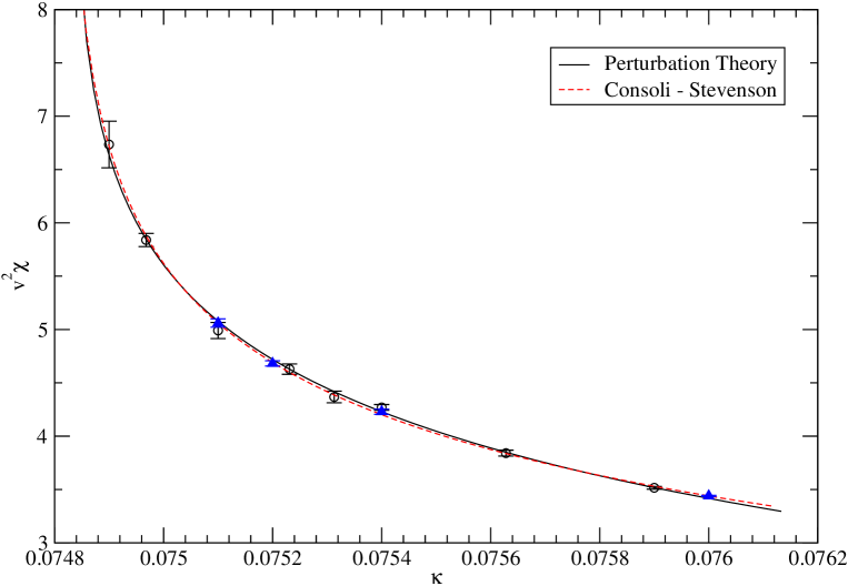
Figure 1: Fits of the data (circles) of Cea et al for $v^{2}\chi$. The triangles are the data of this investigation.

5 Field theory simulations at constant physics

We have also studied the cutoff dependence of the renormalization constant $Z_{{\hbox{\sixrm R}}}$ along a line of constant IR physics, keeping the renormalized coupling $g_{{\hbox{\sixrm R}}}$ (defined in Eq. (2.10)) fixed as the renormalized mass $m_{{\hbox{\sixrm R}}}$ in lattice units is varied. This is of course the behavior of interest in deciding how limits on the appearance of new UV physics follows from the triviality of the lattice model in the continuum limit. This has been done at three points $\bar{\lambda}=0.3,0.6$ and 1.0 (the Ising limit) along the RG curve corresponding to $g_{{\hbox{\sixrm R}}}\simeq 20$ (cf Fig. 2 of [?]). The simulations in the field theory cases ($\bar{\lambda}=0.3,0.6$) were done with conventional Metropolis update code on lattices of size $64^{4}$, while the Ising point results were obtained using a cluster code on lattices of size $48^{4}$.

The renormalization constant $Z_{{\hbox{\sixrm R}}}$ and the zero momentum renormalized mass $m_{{\hbox{\sixrm R}}}$ were extracted from a fit of the inverse lattice propagator in momentum space for small lattice momenta:

$$\tilde{G}(k)^{-1}=Z_{{\hbox{\sixrm R}}}^{-1}(m_{{\hbox{\sixrm R}}}^{2}+\hat{k}^{2}+{\rm O}(k^{4}))\,.$$ (5.27)

In the cases ($\bar{\lambda}=0.3$, $0.6$), we have computed $G(k)=\langle|\phi(k)|^{2}\rangle$ from the FFT (fast-Fourier-transform) $\phi(k)$ of the coordinate space field $\phi(x)$. The FFT is performed every 40 Monte-Carlo sweeps: we find that the nonzero momentum modes of $\tilde{G}(k)$, for which the vev is irrelevant, have an autocorrelation time ranging from 50 to a few hundred sweeps. For $\bar{\lambda}$=0.3 we have collected propagators for a total of 50K sweeps (1250 propagators), while for $\bar{\lambda}=$0.6 we have 100K sweeps (2500 propagators).

Only the lowest $4^{4}$-1=255 modes are included in the fit: the mode corresponding to zero momentum is omitted. We then perform an uncorrelated (diagonal chi-square) fit of the 34 data points (corresponding to different values of $\hat{k}^{2}$) to Eq. (5.27). The chi-squared/degree of freedom for the $\bar{\lambda}=$0.3 (resp. 0.6) point was 40/32 (resp. 54/32). The results for $Z_{{\hbox{\sixrm R}}},m_{{\hbox{\sixrm R}}}$ obtained by this procedure are indicated in Table 5. Also shown is the field vacuum expectation value (unrenormalized) $\langle\phi\rangle$, from which a renormalized coupling $g_{{\hbox{\sixrm R}}}$, also shown in the Table, can be obtained. Finally, we give the susceptibility $\chi$ and the value $2\kappa m_{{\hbox{\sixrm R}}}^{2}\chi$ which is the value of $Z_{{\hbox{\sixrm R}}}$ calculated from the zero momentum propagator, Eq. (2.5).

It is apparent from the results in Table 5 that the cutoff dependence of $Z_{{\hbox{\sixrm R}}}$ is extremely mild over the entire range covering a factor of 3 in cutoff holding the physical mass fixed, perfectly in accord with conventional renormalization wisdom. Note that the values of $2\kappa m_{{\hbox{\sixrm R}}}^{2}\chi$ agree with the latter determination of $Z_{{\hbox{\sixrm R}}}$ within the errors, as it should be since the Fourier transform of the (subtracted) correlator, $\tilde{G}(k)$ is a continuous function. This again shows that the determination of the bare vev is correct.

$\bar{\lambda}$	$\,\,\,\,\,\,\lambda$	$\,\,\,\,\,\,\,\,\kappa$	$\,\,\,\,\,\,\,\,\,\,v$	$\,\,\,\,\,\,\,m_{{\hbox{\sixrm R}}}$
0.3	0.275376	0.144499	0.36895(2)	0.5216(48)
0.6	1.177242	0.130307	0.13957(13)	0.1873(15)
1.0	$\infty$	0.0751	0.15657(4)	0.1691(15)
$\bar{\lambda}$	$\,\,\,\,\,\,\,\,\widehat{Z_{{\hbox{\sixrm R}}}}$	$\,\,\,\,\,g_{{\hbox{\sixrm R}}}$	$\,\,\,\,\,\,\,\chi$	$\,\,\,\,\,2\kappa m_{{\hbox{\sixrm R}}}^{2}\chi$
0.3	0.962(12)	20.2(4)	12.40(5)	0.975(20)
0.6	0.951(4)	19.7(4)	102.5(3.5)	0.937(48)
1.0	0.896(8)	20.6(7)	206.4(1.2)	0.886(17)

Table 5: Results for simulations on the RG curve, $g_{{\hbox{\sixrm R}}}\simeq 20$

As there may be some question of the extent to which the inverse momentum space propagator is adequately fit by Eq. (5.27) with two parameters, we have displayed the quality of the fits for $\bar{\lambda}$=0.3, 0.6 in Figures 2, 3. There is certainly no evidence for any curvature up to the maximum momenta included in the fit, and indeed the chi-square/degree of freedom for the two-parameter fit is perfectly fine. In Table 5 for the Ising case we quote numbers for $m_{{\hbox{\sixrm R}}}$ and $Z_{{\hbox{\sixrm R}}}$, obtained by fitting the first three $k\neq 0$ values (with $k$ along the time-axis) of the inverse propagator. These numbers differ only slightly from those given (for the same $\kappa$) in Table 4 using the alternative method of extraction described in the previous section. We remark that in this case (as one can check using Table 2) the inverse propagator is remarkably linear in $\hat{k}^{2}$ up to the maximal (on-axis) momentum $\hat{k}^{2}=4$.

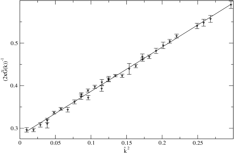
Figure 2: $[2\kappa\tilde{G}(k)]^{-1}$ at $\bar{\lambda}$=0.3, $g_{{\hbox{\sixrm R}}}\simeq 20$. The triangles are the data from 50K sweeps 1250 propagators. The fit is with $\widehat{Z_{{\hbox{\sixrm R}}}},m_{{\hbox{\sixrm R}}}$ given in Table 5.

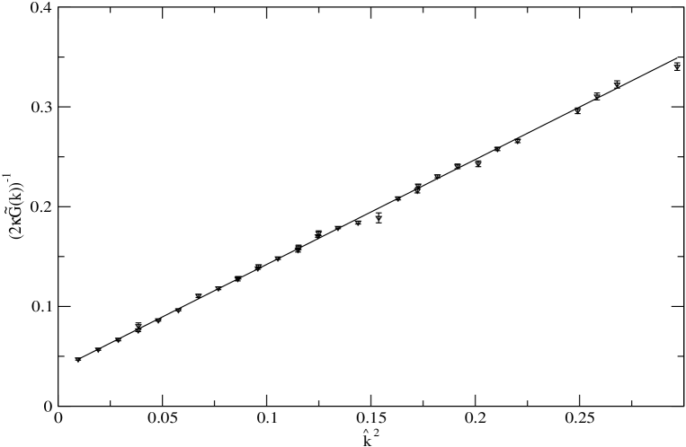
Figure 3: $[2\kappa\tilde{G}(k)]^{-1}$ at $\bar{\lambda}$=0.6, $g_{{\hbox{\sixrm R}}}\simeq 20$. The triangles are the data from 100K sweeps 2500 propagators. The fit is with $\widehat{Z_{{\hbox{\sixrm R}}}},m_{{\hbox{\sixrm R}}}$ given in Table 5.

6 Conclusions

In this paper we have shown that simulation data is in perfect agreement with the conventional renormalization group scenario in the lattice 1-component $\phi^{4}_{4}$ model. This is contrary to the claim of ref. [?]. We have explained the deficiencies in their analysis. The quantitative agreement with analytically obtained results is completely satisfactory taking into account that some systematic errors are probably underestimated in ref. [?].

Conventional wisdom is not firmly established merely by a majority vote, but on solid theoretical and numerical studies. The same applies of course to deeper questions e.g. whether QCD is the correct theory of hadronic physics. The work reported here again reinforces the CW regarding triviality. Had the critique of the authors [?] been correct, they would have indicated serious non-standard implications concerning the Higgs’ sector of the Standard Model.

6.1 Acknowledgments

We thank the Leibniz-Rechenzentrum where part of the computations were carried out. This investigation was supported in part by the Hungarian National Science Fund OTKA (under T034299 and T043159) and by the Schweizerischer Nationalfonds. The work of A. Duncan was supported in part by NSF grant PHY-0244599.

References

- [1] P. Cea, M. Consoli, L. Cosmai, hep-lat/0407024
- [2] M. Lüscher, P. Weisz, Nucl. Phys. B290 (1987) 25
- [3] M. Lüscher, P. Weisz, Nucl. Phys. B295 (1988) 65
- [4] E. Brézin, J. C. Le Guillou, J. Zinn-Justin, “Field theoretical approach to critical phenomena”, Vol.6, Eds. C. Domb and M. S. Green, Academic Press, London (1976)
- [5] D. S. Gaunt, M. F. Sykes, S. McKenzie, J. Phys. A12 (1979) 871
- [6] D. Stauffer, J. Adler, Int. J. Mod. Phys. C8 (1997) 263
- [7] R. Kenna, C. B. Lang, Nucl. Phys. B393 (1993) 461; Erratum-ibid. B411 (1994) 340
- [8] C. Vohwinkel, P. Weisz, Nucl. Phys. B374 (1992) 647
- [9] Letter from P. Hasenfratz to the authors of [?], Sept.1988
- [10] M. Lüscher, P. Weisz, Nucl. Phys. B318 (1989) 705
- [11] R. H. Swendsen, J.-S. Wang, Phys. Rev. Lett. 58 (1987) 86
- [12] K. Jansen, T. Trappenberg, I. Montvay, G. Münster, U. Wolff, Nucl. Phys. B322 (1989) 698
- [13] K. Binder, Z. Phys. B43 (1981) 119