Twisted mass QCD for the pion electromagnetic form factor

Abstract

The pion form factor is computed using quenched twisted mass QCD and the GMRES-DR matrix inverter. The momentum averaging procedure of Frezzotti and Rossi is used to remove leading lattice spacing artifacts, and numerical results for the form factor show the expected improvement with respect to the standard Wilson action. Although some matrix inverters are known to fail when applied to twisted mass QCD, GMRES-DR is found to be a viable and powerful option. Results obtained for the pion form factor are consistent with the published results from other $O(a)$ improved actions and are also consistent with the available experimental data.

I Overview and discussion

The Wilson lattice action for fermionsWilson does not have exact chiral symmetry, and thus it provides no lower bound for the norm of Dirac matrix eigenvalues. As a practical consequence, numerical simulations encounter “exceptional configurations” (for which the Dirac matrix cannot be inverted) with increasing regularity as the quark mass is reduced. Symanzik improvement of the Wilson action by adding the Sheikholeslami-Wohlert term with a properly tuned coefficientclover , exacerbates the problem.

Fortunately, the addition of a twisted mass term provides a lower bound for the eigenvalues thereby eliminating exceptional configurations.tmQCD ; FreLat04 Furthermore, tuning of the Sheikholeslami-Wohlert coefficient is no longer needed for the removal of linear lattice spacing errors. Instead, many quantities are automatically improved simply by adding the twisted mass term to the basic Wilson action and setting the hopping parameter to its critical value (i.e. $\kappa=\kappa_{c}$ in Eq. (13) below), while other quantities become improved by averaging over equal and opposite momenta.FreRos ; FreLat04 The present work provides an explicit numerical verification of the averaging technique for improvement in twisted mass QCD (tmQCD).

Our discussion will focus on the pion electromagnetic form factor. Due to the simple valence quark structure of the pion and a firm theoretical knowledge of its form factor in both the $Q^{2}\to 0$ and $Q^{2}\to\infty$ limits, the pion form factor is a preferred place to study the transition between perturbative and nonperturbative QCD. Experimental studies are ongoing at Jefferson Lab, and theoretical modelling is also continuing.experiment

Initial studies of the pion form factor using lattice QCD occurred some time ago,firstlat ; Draper and new lattice initiatives have arisen recently for Wilson, Sheikoleslami-Wohlert, and domain wall actions.LHPC ; vanderH ; Nemoto Preliminary results from our tmQCD study were presented in Ref. ourprelim . In contrast to other form factors, the pion form factor receives no contributions from the vector current attaching to a nonvalence quark (so-called “disconnected diagrams”), and this feature reduces the lattice QCD cost considerably.Draper There could still be contributions from sea quarks that do not interact directly with the external vector current, and these have been considered in Ref. dynapion where dynamical configurations were to used obtain the pion form factor. All other studies to date, including the present one, have used the quenched approximation and thereby omitted all nonvalence quarks.

In the remainder of this article, we report on our use of quenched tmQCD to compute the pion form factor. Two quark masses corresponding to pion masses near 470 MeV and 660 MeV, as well as a variety of momentum transfer values satisfying 0 GeV${}^{2}<Q^{2}\lesssim 5$ GeV² have been considered, all at a lattice spacing of 0.10 fm. A comparison to existing lattice results clearly shows the improvement expected for tmQCD, since the momentum-averaged tmQCD data agree with results from other improved actions and differ from unimproved Wilson results at this same lattice spacing. Interestingly, even before momentum averaging the tmQCD data are closer to improved action results than to unimproved Wilson results for this particular observable, despite the fact that the pion form factor technically requires momentum averaging to exactly remove the linear lattice spacing errors.

To determine the renormalization factors that appear in the pion form factor correlation function, and to compare with the predictions of vector meson dominance, we also study two-point pseudoscalar and vector correlators with nonzero momenta. The associated dispersion relations are compared to continuum expectations as another means of exploring lattice spacing artifacts.

One of the technical issues that arises in tmQCD simulations is the failure of some standard matrix inversion algorithms. Alternative algorithms are being used and evaluated by various authors.inverters The present work makes use of the GMRES-DR algorithmGMRESDR and concludes that it performs well for tmQCD. Some details are presented in Section IV.

This initial exploration of the pion form factor with tmQCD leads to optimism that future lattice tmQCD studies, perhaps with smeared operators and increased statistics on larger lattices, can reach smaller quark masses with greater precision. Our present results are consistent with vector meson dominance and with experiment. More generally, the present work underscores the value of lattice tmQCD itself as a practical tool for hadron phenomenology.

II Correlation functions

The electromagnetic form factor of a charged pion is defined by

$$\left<\pi^{+}(\vec{p}_{f})|j_{\mu}(0)|\pi^{+}(\vec{p}_{i})\right>=F(Q^{2})(p_{i}+p_{f})_{\mu}$$ (1)

where $j_{\mu}(0)$ is a conserved vector current evaluated at the spacetime origin, $p_{i}$ and $p_{f}$ are the initial and final pion (Euclidean) 4-momenta respectively, $\vec{p}_{i}$ and $\vec{p}_{f}$ are the corresponding 3-momenta, and $Q^{2}=(p_{f}-p_{i})^{2}$ is the 4-momentum transfer. To compute this matrix element on a spacetime lattice, one can use the three-point correlator displayed in Fig. 1. A source with pion quantum numbers is placed at $x_{i}$, a sink at $x_{f}$, and a vector current is inserted at $x$. Given an interpolating field operator $\phi(x)$ with the quantum numbers of the charged pion, one can extract the form factor from the following three-point correlator:

$$\Gamma_{\pi\mu\pi}(t_{i},t,t_{f},\vec{p}_{i},\vec{p}_{f})=\sum_{\vec{x}_{i},\vec{x}_{f}}e^{-i(\vec{x}_{f}-\vec{x})\cdot\vec{p}_{f}}e^{-i(\vec{x}-\vec{x}_{i})\cdot\vec{p}_{i}}\left<0|\phi(x_{f})j_{\mu}(x)\phi^{\dagger}(x_{i})|0\right>.$$ (2)

Note that we are working in units of lattice spacing throughout this discussion. In this work we choose $\phi(x)$ to be the local operator

$$\phi(x)=\bar{d}(x)\gamma_{5}u(x)$$ (3)

where $u(x)$ and $d(x)$ are the up and down quark fields respectively. Smeared operators could be of value in subsequent studies, particularly for the exploration of the high $Q^{2}$ range. For the vector current, $j_{\mu}(x)$, we use the conserved current,

$$j_{\mu}(x)=\frac{1}{2}\bar{u}(x)(1-\gamma_{\mu})U_{\mu}(x)u(x+\hat{\mu})-\frac{1}{2}\bar{u}(x+\hat{\mu})(1+\gamma_{\mu})U_{\mu}^{\dagger}(x)u(x)$$ (4)

with $\mu=4$. In order to extract the matrix element in Eq. (1) from the three-point correlator of Eq. (2), one introduces two complete sets of states $|n(\vec{k})\rangle$ with the same quantum numbers as $\phi(x)$ in the three-point correlator and gets

$$\Gamma_{\pi\mu\pi}(t_{i},t,t_{f},\vec{p}_{i},\vec{p}_{f}) = \sum_{n}\sum_{m}\left<0|\phi(x)|m(\vec{p}_{f})\right>{{e^{-(t_{f}-t)E_{m}(\vec{p}_{f})}}\over{2E_{m}(\vec{p}_{f})}}\left<m(\vec{p}_{f})|j_{\mu}(x)|n(\vec{p}_{i})\right>$$ (5)

$${{e^{-(t-t_{i})E_{n}(\vec{p}_{i})}}\over{2E_{n}(\vec{p}_{i})}}\left<n(\vec{p}_{i})|\phi^{\dagger}(x)|0\right>.$$

This can be simplified further using

$$\left<0|\phi(x)|m(\vec{p})\right>=Z_{m}(\vec{p})e^{ix\cdot p}$$ (6)

and for a local interpolating field operator, $Z_{m}(\vec{p})$ is independent of $\vec{p}$. The three-point correlator simplifies to

$$\Gamma_{\pi\mu\pi}(t_{i},t,t_{f},\vec{p}_{i},\vec{p}_{f})=\sum_{n}\sum_{m}Z_{m}{{e^{-(t_{f}-t)E_{m}(\vec{p}_{f})}}\over{2E_{m}(\vec{p}_{f})}}\left<m(\vec{p}_{f})|j_{\mu}(0)|n(\vec{p}_{i})\right>{{e^{-(t-t_{i})E_{n}(\vec{p}_{i})}}\over{2E_{n}(\vec{p}_{i})}}Z_{n}^{*}.$$ (7)

Similarly the two-point correlator, which will be needed to get the energies, is given by

$$G_{\pi\pi}(t_{i},t,\vec{p})=\sum_{\vec{x}}e^{-i(\vec{x}-\vec{x}_{i})\cdot\vec{p}}\left<0|\phi(x)\phi^{\dagger}(x_{i})|0\right>=\sum_{n}Z_{n}Z_{n}^{*}{{e^{-(t-t_{i})E_{n}(\vec{p})}}\over{2E_{n}(\vec{p})}}.$$ (8)

For periodic boundary conditions on a lattice of $N_{t}$ time slices, Eq. (8) will be modified to

$$G_{\pi\pi}(t_{i},t,\vec{p})=\sum_{n}\frac{Z_{n}Z_{n}^{*}}{E_{n}(\vec{p})}e^{-\left(\frac{N_{t}}{2}\right)E_{n}(\vec{p})}\cosh\left[\left(t-t_{i}-\frac{N_{t}}{2}\right)E_{n}(\vec{p})\right].$$ (9)

The long time behaviour of the two and three-point correlators will be dominated by contributions from the lightest pseudoscalar state, i.e. the pion. This asymptotic behaviour is given by

$$\Gamma_{\pi\mu\pi}(t_{i},t,t_{f},\vec{p}_{i},\vec{p}_{f}) \stackrel{{\scriptstyle t_{f}\gg t\gg t_{i}}}{{\longrightarrow}} |Z_{\pi}|^{2}\frac{e^{-(t-t_{i})E_{\pi}(\vec{p}_{i})-(t_{f}-t)E_{\pi}(\vec{p}_{f})}}{4E_{\pi}(\vec{p}_{i})E_{\pi}(\vec{p}_{f})}F(Q^{2})(p_{i}+p_{f})_{\mu},$$ (10)

$$G_{\pi\pi}(t_{i},t,\vec{p}) \stackrel{{\scriptstyle|t-t_{i}|\gg 0}}{{\longrightarrow}} \frac{|Z_{\pi}|^{2}}{E_{\pi}(\vec{p})}e^{-\left(\frac{N_{t}}{2}\right)E_{\pi}(\vec{p})}\cosh\left[\left(t-t_{i}-\frac{N_{t}}{2}\right)E_{\pi}(\vec{p})\right].$$ (11)

To obtain a reliable result for the pion form factor, we will allow for contributions from excited states. For the conserved current, the corresponding transition matrix elements are included as follows,

$$\left<\pi_{\beta}(\vec{p}_{f})|j_{\mu}(0)|\pi_{\alpha}(\vec{p}_{i})\right>=F_{\alpha\beta}(Q^{2})\left[(p_{f}+p_{i})_{\mu}-\frac{(p_{f}^{2}-p_{i}^{2})}{(p_{f}-p_{i})^{2}}(p_{f}-p_{i})_{\mu}\right].$$ (12)

III The action and its parameters

Our simulations use the standard Wilson gauge action with $\beta=6.0$. An ensemble of 100 quenched configurations of size $16^{3}\times 48$ was created using a pseudo-heatbath algorithm, with 5000 sweeps omitted between saved configurations. The lattice tmQCD fermion action is

$$S_{F}[\psi,\bar{\psi},U]=\sum_{x}\bar{\psi}(x)\left[1+2\kappa\mu i\gamma_{5}\tau_{3}+\kappa\sum_{\nu}\gamma_{\nu}\left(\nabla_{\nu}+\nabla^{*}_{\nu}-\nabla^{*}_{\nu}\nabla_{\nu}\right)\right]\psi(x)$$ (13)

where the forward and backward lattice derivatives are defined as usual,

$$\nabla_{\nu}\psi(x) \equiv U_{\nu}(x)\psi(x+\hat{\nu})-\psi(x),$$ (14)

$$\nabla_{\nu}^{*}\psi(x) \equiv \psi(x)-U_{\nu}^{\dagger}(x-\hat{\nu})\psi(x-\hat{\nu}),$$ (15)

and $\psi(x)$ denotes the doublet of up and down quarks. When $\mu=0$, $S_{F}$ becomes the standard Wilson action. Throughout this work, we hold the hopping parameter fixed at its critical value, $\kappa_{c}=0.156911$,XLFscaling leaving the quark mass directly proportional to $\mu$. Our pion form factor studies are carried out with $\mu=0.030$ and $\mu=0.015$. We also choose the temporal separation of the source and sink to be $t_{f}-t_{i}=15$ time steps. The additional cases of $\mu=0.007$, 0.003 and 0.001 are used below as insightful exercises for GMRES-DR. Periodic boundary conditions are used in all directions.

Frezzotti and Rossi have shown that, when the hopping parameter is set to its critical value (so-called “maximal twist”), masses and correlation functions with vanishing spatial momenta are automatically $O(a)$ improved in tmQCD.FreRos A generic matrix element with non-zero spatial momenta can be improved by averaging over momenta of equal magnitude but opposite sign as follows,

$$\left<f,\vec{k}|B|i,\vec{p}\right>+\eta_{i,f,B}\left<f,-\vec{k}|B|i,-\vec{p}\right>=2\xi_{B}\left<f,\vec{k}|B|i,\vec{p}\right>|_{{\rm continuum}}+O(a^{2})$$ (16)

where $\eta_{i,f,B}=\pm 1$ is an overall parity (see Ref. FreRos for the precise definition of this parity) for the matrix element between the initial state $|i,\vec{p}\rangle$, the final state $|f,\vec{k}\rangle$, and the operator $B$. The renormalization coeffecient $\xi_{B}$ relates the continuum and lattice operators. Since the energies obtained from a two-point correlator depend only on $|\vec{k}|^{2}$ these energies, like masses, are automatically improved without momentum averaging.

IV Matrix inversion

Some of the standard matrix inverters used in lattice QCD research, such as the stabilized biconjugate gradient, fail when applied to tmQCD at maximal twist for sufficiently light quarks.inverters Fortunately there are other inversion algorithms that succeed for tmQCD inversions, such as conjugate gradient, conjugate gradient squared and GMRES.inverters The present work made use of the GMRES-DR algorithmGMRESDR , and the remainder of this section contains some information about our experience with this inverter.

The GMRES-DR inverter is built on the standard GMRES (generalized minimal residual) matrix inverter, but extends it to incorporate deflation (D) of the smallest eigenvalues even after subsequent restarts (R) of the basic GMRES algorithm. Since GMRES-DR is a significant improvement over standard GMRES, and since standard GMRES can successfully invert tmQCD matrices, it is interesting to explore the application of GMRES-DR to tmQCD.

GMRES uses a Krylov vector space of some dimensionality (let’s call it $n$) chosen by the user and GMRES-DR identifies and retains the $k$-dimensional subspace spanned by light eigenvectors, where $k$ is also chosen by the user. For the present work, $n$ and $k$ were chosen to minimize the wall clock time needed to reach a residual of $|r|<10^{-6}$, where $r\equiv b-Mx$ for Dirac matrix $M$ and source vector $b$. This optimization was done at $\kappa=\kappa_{c}$ and $\mu=0.030$ and for our implementation of GMRES-DR($n$,$k$) the result was $(n,k)=(40,10)$.

For our ensemble of 100 configurations, all GMRES-DR(40,10) inversions were successful at $\mu=0.030$, 0.015 and 0.007. The pion form factor was not computed at $\mu=0.007$ due to the onset of finite volume effects, but the pseudoscalar two-point correlator was computed for $\mu\leq 0.007$ as a means of gaining some experience with GMRES-DR. At $\mu=0.003$, GMRES-DR(40,10) failed to compute one column out of 1200 but increasing the Krylov subspace to GMRES-DR(60,10) brought success. At $\mu=0.001$, GMRES-DR(40,10) failed to compute three columns out of 1200 but GMRES-DR(60,10) was again completely successful. Recall that our choice of $(n,k)=(40,10)$ arose from optimization at $\mu=0.030$; we did not optimize separately at these very small $\mu$ values.

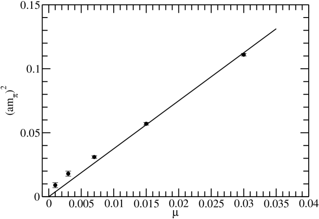
Figure 2: Pseudoscalar mass versus the twisted quark mass parameter $\mu$. The solid curve is a fit of the data at $\mu=0.030$ and $0.015$ to a straight line through the origin. Data points below $\mu=0.007$ were computed for the exploration of GMRES-DR, not for phenomenological use.

Table 1 displays the average number of matrix-vector products that were computed to obtain one column of the inverse to a residual of $|r|<10^{-6}$ using GMRES-DR(40,10). Since this number of matrix-vector products depends on our particular source (i.e. a point source with specific color index and Dirac index) and also on our particular initial value for the solution vector, it is more useful to report the change in $|r|$ relative to its initial (i.e. before any GMRES-DR iterations) value. In the present case, the initial residual was $|r_{0}|=40.62$ so the data in Table 1 represent the number of matrix-vector products computed to reach $|r/r_{0}|<2.5\times 10^{-8}$. This is the quantity that can be meaningfully compared to studies with other source vectors.multiRHS Figure 2 shows the pseudoscalar mass squared as a function of $\mu$ as well as the result of fitting the two largest $\mu$ data points to a straight line through the origin. Finite volume effects are apparent for $\mu\leq 0.007$.

V Results

We first analyze the pseudoscalar and vector two-point correlators. Energies are obtained by fitting the pseudoscalar correlators to Eq. (9) and the vector correlators to the analogous expression. Spatial components of nonzero momenta are averaged over all spatial directions to improve statistics; the three spatial components of the vector operator are also averaged.

Single state fits to the data show a convincing ground state signal for $|\vec{p}|^{2}\leq 4p_{{\rm min}}^{2}$, where $p_{{\rm min}}=2\pi/L$ and $L=16$ is the spatial size of our lattice. Multi-state fits were also performed, and led to consistent results for the ground state energies. These results can be compared to the predictions of the continuum and lattice dispersion relations given by

$$(aE_{cont.})^{2} = (aM)^{2}+|\vec{p}|^{2},$$ (17)

$$\sinh^{2}\left(\frac{aE_{latt.}}{2}\right) = \sinh^{2}\left(\frac{aM}{2}\right)+\sum_{i=1}^{3}\sin^{2}\left(\frac{p_{i}}{2}\right),$$ (18)

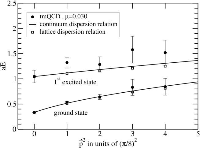
Figure 3: Ground state and first excited state pseudoscalar meson energies from three-state fits to tmQCD at $\mu=0.030$, as compared to the continuum and lattice dispersion relations.

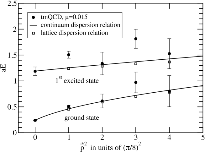
Figure 4: Ground state and first excited state pseudoscalar meson energies from three-state fits to tmQCD at $\mu=0.015$, as compared to the continuum and lattice dispersion relations.

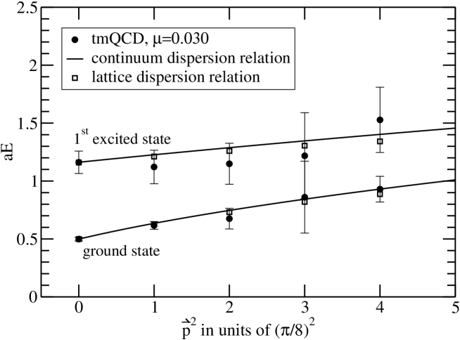
Figure 5: Ground state and first excited state vector meson energies from three-state fits to tmQCD at $\mu=0.030$, as compared to the continuum and lattice dispersion relations.

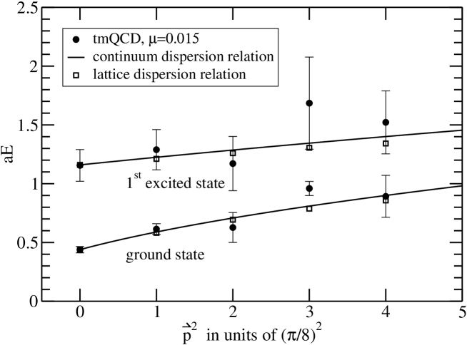
Figure 6: Ground state and first excited state vector meson energies from three-state fits to tmQCD at $\mu=0.015$, as compared to the continuum and lattice dispersion relations.

respectively. Figures 3, 4, 5 and 6 show this comparison where the mass parameters in Eqs. (17) and (18) were chosen to match the lattice data at $\vec{p}=\vec{0}$. Table 2 contains the numerical values of the pion and $\rho$ meson masses at those two values of $\mu$ for which the pion form factor is calculated.

To extract the pion form factor, we performed a simultaneous fit over the pseudoscalar two-point correlator with momentum $\vec{p}_{i}$, the pseudoscalar two-point correlator with momentum $\vec{p}_{f}$, and the pseudoscalar($\vec{p}_{i}$)-vector-pseudoscalar($\vec{p}_{f}$) three-point correlator. The fourth component of the conserved vector current was used. To verify the stability of the ground state, we’ve performed both a single state fit over the large time ranges of the two-point and three-point correlators where the ground state pion dominates using Eqs. (10) and (11), and a three state fit over the entire time range (except the source time step) where the ground state pion as well as first and second excited states are included. This latter method involves $3^{2}=9$ form factors, $F_{\alpha\beta}$, from Eq. (12). For clarity, here are the explicit forms of the correlators used for the three state fit:

$$G_{\pi\pi}^{initial}(t_{i},t,\vec{p}_{i})=\sum_{n=1}^{3}\frac{Z_{n}^{i}{Z_{n}^{i}}^{*}}{E_{n}(\vec{p}_{i})}e^{-\left(\frac{N_{t}}{2}\right)E_{n}(\vec{p}_{i})}\cosh\left[\left(t-t_{i}-\frac{N_{t}}{2}\right)E_{n}(\vec{p}_{i})\right],$$ (19)

$$G_{\pi\pi}^{final}(t_{i},t,\vec{p}_{f})=\sum_{n=1}^{3}\frac{Z_{n}^{f}{Z_{n}^{f}}^{*}}{E_{n}(\vec{p}_{f})}e^{-\left(\frac{N_{t}}{2}\right)E_{n}(\vec{p}_{f})}\cosh\left[\left(t-t_{i}-\frac{N_{t}}{2}\right)E_{n}(\vec{p}_{f})\right],$$ (20)

$$\Gamma_{\pi\mu\pi}(t_{i},t,t_{f},\vec{p}_{i},\vec{p}_{f})=\sum_{n=1}^{3}\sum_{m=1}^{3}Z_{m}^{f}{{e^{-(t_{f}-t)E_{m}(\vec{p}_{f})}}\over{2E_{m}(\vec{p}_{f})}}\left<\pi_{m}(\vec{p}_{f})|j_{\mu}(0)|\pi_{n}(\vec{p}_{i})\right>{{e^{-(t-t_{i})E_{n}(\vec{p}_{i})}}\over{2E_{n}(\vec{p}_{i})}}{Z_{n}^{i}}^{*}.$$ (21)

As will be shown, the ground state is quite stable regardless of whether the single state fit or three state fit is used. The intermediate case of fitting to a ground state plus one excited state leads to similar results, and will not be discussed further.

For the single state fit, the fitting parameters are the energies $E$, the prefactors $Z$, and the form factor $F(Q^{2})$ from Eqs. (10) and (11). For the three state fit, the fitting parameters are the energies $E$ and prefactors $Z$ from Eqs. (19), (20) and (21) as well as the form factors $F(Q^{2})$ and $F_{\alpha\beta}$ from Eqs. (1) and (12). A standard unconstrained $\chi^{2}$ minimization fitting procedure was used. Results from a single state fit to the large (Euclidean) time region were found to be consistent with results from a three state fit beginning just one time step from the source.

Various choices for $\vec{p}_{i}$ and $\vec{p}_{f}$ correspond to comparable momentum transfers, $Q^{2}$, but the cleanest data come when $|\vec{p}_{i}|$ and $|\vec{p}_{f}|$ are minimal. It is therefore not desirable to restrict oneself exclusively to $\vec{p}_{f}=\vec{0}$. For $\mu=0.015$ we have computed with $\vec{p}_{f}=(0,0,\pm p_{min})$ as well as $\vec{p}_{f}=\vec{0}$. For $\mu=0.030$ we only computed with $\vec{p}_{f}=(0,0,\pm p_{min})$. Each new value of $\vec{p}_{f}$ required a new matrix inversion, since the calculation was performed by combining the propagator from $x_{i}$ to $x$ with the sequential propagator from $x_{i}$ to $x_{f}$ to $x$. (See Fig. 1.) All values of $\vec{p}_{i}$ that produce the same $\vec{q}$ were averaged. Finally, the momentum averaging procedure of Eq. (16) was employed to remove $O(a)$ errors.

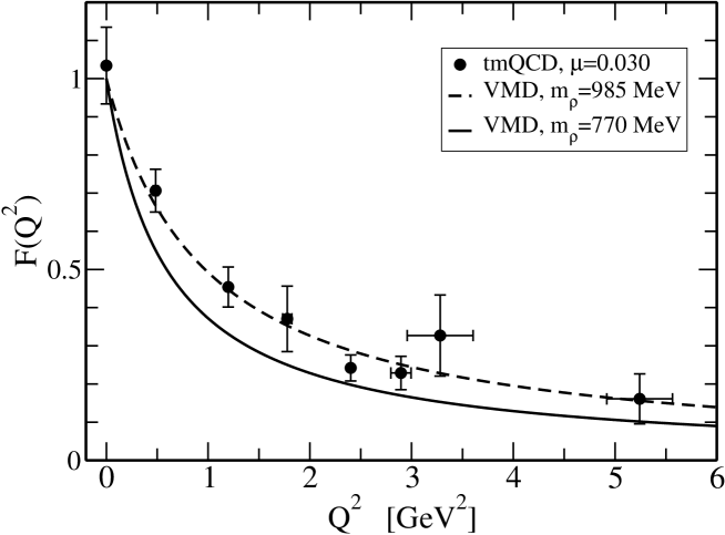
Figure 7: The form factor at $\mu=0.030$ obtained from single state fitting as compared to vector meson dominance.

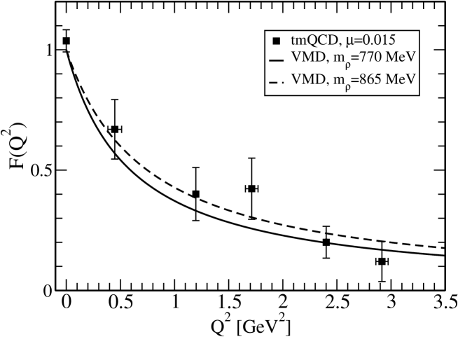
Figure 8: The form factor at $\mu=0.015$ obtained from single state fitting as compared to vector meson dominance.

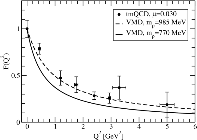
Figure 9: The form factor at $\mu=0.030$ obtained from three state fitting as compared to vector meson dominance.

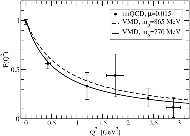
Figure 10: The form factor at $\mu=0.015$ obtained from three state fitting as compared to vector meson dominance.

In Tables 3 and 4 we show the results for the pion form factor obtained from one state fits at $\mu=0.030$ and $0.015$ respectively. These same data are displayed graphically in Figs. 7 and 8. The physical scale was set to $a=0.10$ fmalat . The data show agreement with the corresponding vector meson dominance curves. Results from three state fitting are completely consistent with the one state fits, as shown in Tables 5 and 6 and Figs. 9 and 10. Notice the advantage of using a conserved current: the normalization of the form factor is $F(0)=1$ without any multiplicative renormalization factor $Z_{V}$.

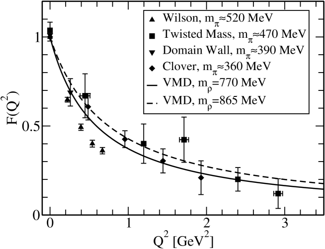
Figure 11: Comparing the quenched tmQCD pion form factor with other quenched lattice calculations (Wilson from Ref. LHPC , clover from Ref. vanderH , domain wall from Ref. Nemoto ) and with vector meson dominance.

In Fig. 11, we compare our results at $\mu=0.015$ to other quenched calculations of the pion form factor at similar quark masses. Two vector meson dominance (VMD) curves are also shown — one with the physical $\rho$ meson mass and the other with the vector meson mass taken from our tmQCD simulation at $\mu=0.015$. The available experimental data are known to follow VMD with the physical $\rho$ meson mass. As evident from Fig. 11, the Wilson results have a large systematic lattice discretization error while the tmQCD results are consistent with other improved action results and with VMD. Since the quark mass in the Wilson simulation of Fig. 11 is somewhat larger than the quark masses in the other simulations, one would expect the Wilson form factor to be slightly larger than the others. The plot clearly shows the opposite effect, suggesting that the $O(a)$ contributions are large. As discussed in Ref. LHPC the apparent smallness of the Wilson form factor is correlated with the smallness of the Wilson vector meson massEdwardsHK . For example, the Wilson form factor would be consistent with VMD if the physical scale (i.e. the lattice spacing needed to compute values of $Q^{2}$ for the horizontal axis in Fig. 11) were obtained from the vector meson mass itself. The tmQCD action does not have large $O(a)$ contributions to the vector meson massXLFscaling and we find correspondingly small $O(a)$ contributions to the pion form factor.

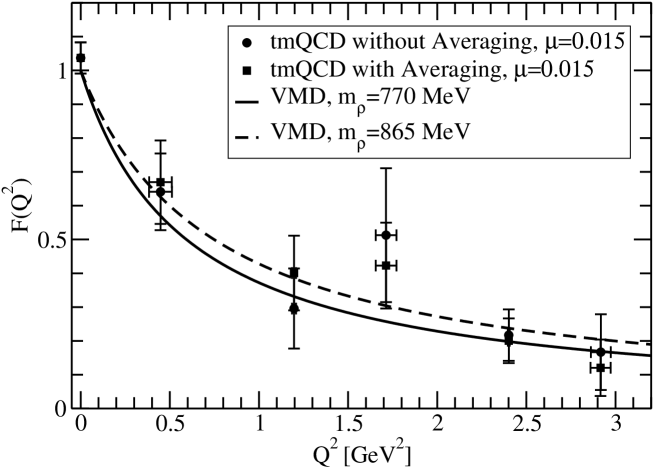
Figure 12: The pion form factor from tmQCD at $\mu=0.015$ with and without momentum averaging.

As discussed above, the tmQCD results are improved through momentum averaging at maximal twist ($\kappa=\kappa_{c}$). Unimproved tmQCD results would be obtained simply by omitting the momentum averaging step. Figure 12 shows the tmQCD pion form factor results at $\mu=0.015$ obtained from a one state fit with and without the averaging procedure. Interestingly, the data are quite consistent within the statistical uncertainties of our simulation.

Table 1: The average number of matrix-vector products required to compute one column of the inverse to a residual of $|r|<(2.5\times 10^{-8})|r_{0}|$ using GMRES-DR(40,10), where $r_{0}$ denotes the initial residual.

$\mu$	average number of products
0.030	816
0.015	1175
0.007	1384
0.003	1450
0.001	1489

Table 2: Ground state pseudoscalar and vector meson masses.

$\mu$	0.015	0.030
$am_{\pi}$	0.240(3)	0.334(2)
$am_{\rho}$	0.439(27)	0.499(15)

Table 3: Momentum components in units of $2\pi/L$ used to extract the pion form factor at $\mu=0.030$ from a single state fit. $O(a)$ improvement has been invoked by averaging over data with $n=1$ and $n=-1$.

$\vec{p}_{f}$ [$\frac{2\pi}{L}$]	$\vec{q}$ [$\frac{2\pi}{L}$]	$Q^{2}$ [${\rm GeV^{2}}$]	$F(Q^{2})$
(0,0,$n$)	(0,0,0)	0	$1.034\pm 0.100$
(0,0,$n$)	(0,0,$-n$)	$0.484\pm 0.025$	$0.706\pm 0.056$
(0,0,$n$)	(0,$\pm 1$,$-n$)	$1.198\pm 0.007$	$0.454\pm 0.052$
(0,0,$n$)	($\pm 1$,$\pm 1$,$-n$)	$1.778\pm 0.045$	$0.370\pm 0.086$
(0,0,$n$)	(0,0,$-2n$)	$2.402\pm 0$	$0.242\pm 0.034$
(0,0,$n$)	(0,$\pm 1$,$-2n$)	$2.896\pm 0.1$	$0.229\pm 0.044$
(0,0,$n$)	($\pm 1$,$\pm 1$,$-2n$)	$3.281\pm 0.323$	$0.327\pm 0.106$
(0,0,$n$)	(0,0,$-3n$)	$5.242\pm 0.323$	$0.161\pm 0.065$

Table 4: Momentum components in units of $2\pi/L$ used to extract the pion form factor at $\mu=0.015$ from a single state fit. $O(a)$ improvement has been invoked by averaging over data with $n=1$ and $n=-1$.

$\vec{p}_{f}$ [$\frac{2\pi}{L}$]	$\vec{q}$ [$\frac{2\pi}{L}$]	$Q^{2}$ [${\rm GeV^{2}}$]	$F(Q^{2})$
(0,0,0)	(0,0,0)	0	$1.037\pm 0.046$
(0,0,0)	(0,0,$\pm 1$)	$0.448\pm 0.063$	$0.669\pm 0.124$
(0,0,$n$)	(0,$\pm 1$,$-n$)	$1.197\pm 0.011$	$0.401\pm 0.110$
(0,0,$n$)	($\pm 1$,$\pm 1$,$-n$)	$1.713\pm 0.059$	$0.423\pm 0.127$
(0,0,$n$)	(0,0,$-2n$)	$2.401\pm 0.005$	$0.200\pm 0.066$
(0,0,$n$)	(0,$\pm 1$,$-2n$)	$2.916\pm 0.056$	$0.120\pm 0.083$

Table 5: Momentum components in units of $2\pi/L$ used to extract the pion form factor at $\mu=0.030$ from a three state fit. $O(a)$ improvement has been invoked by averaging over data with $n=1$ and $n=-1$.

$\vec{p}_{f}$ [$\frac{2\pi}{L}$]	$\vec{q}$ [$\frac{2\pi}{L}$]	$Q^{2}$ [${\rm GeV^{2}}$]	$F(Q^{2})$
(0,0,$n$)	(0,0,0)	0	$1.0\pm 0.091$
(0,0,$n$)	(0,0,$-n$)	$0.436\pm 0.038$	$0.787\pm 0.059$
(0,0,$n$)	(0,$\pm 1$,$-n$)	$1.197\pm 0$	$0.473\pm 0.077$
(0,0,$n$)	($\pm 1$,$\pm 1$,$-n$)	$1.756\pm 0.063$	$0.401\pm 0.085$
(0,0,$n$)	(0,0,$-2n$)	$2.394\pm 0$	$0.283\pm 0.041$
(0,0,$n$)	(0,$\pm 1$,$-2n$)	$2.94\pm 0.042$	$0.258\pm 0.055$
(0,0,$n$)	($\pm 1$,$\pm 1$,$-2n$)	$3.294\pm 0.235$	$0.37\pm 0.124$
(0,0,$n$)	(0,0,$-3n$)	$5.0\pm 0.257$	$0.188\pm 0.134$

Table 6: Momentum components in units of $2\pi/L$ used to extract the pion form factor at $\mu=0.015$ from a three state fit. $O(a)$ improvement has been invoked by averaging over data with $n=1$ and $n=-1$.

$\vec{p}_{f}$ [$\frac{2\pi}{L}$]	$\vec{q}$ [$\frac{2\pi}{L}$]	$Q^{2}$ [${\rm GeV^{2}}$]	$F(Q^{2})$
(0,0,0)	(0,0,0)	0	$0.983\pm 0.026$
(0,0,0)	(0,0,$\pm 1$)	$0.429\pm 0.055$	$0.563\pm 0.055$
(0,0,$n$)	(0,$\pm 1$,$-n$)	$1.197\pm 0$	$0.332\pm 0.138$
(0,0,-1)	($\pm 1$,$\pm 1$,$-n$)	$1.751\pm 0.171$	$0.44\pm 0.218$
(0,0,-1)	(0,0,$-2n$)	$2.394\pm 0$	$0.212\pm 0.092$
(0,0,-1)	(0,$\pm 1$,$-2n$)	$2.89\pm 0.141$	$0.115\pm 0.104$

Figure 1: Three-point correlator for the pion form factor.