Abstract

The structure of QCD vacuum can be studied from first principles using the lattice-regularized theory. This line of research entered a qualitatively new phase recently, wherein the space-time structure (at least for some quantities) can be directly observed in configurations dominating the QCD path integral, i.e. without any subjective processing of typical configurations. This approach to QCD vacuum structure does not rely on any proposed picture of QCD vacuum but rather attempts to characterize this structure in a model-independent manner, so that a coherent physical picture of the vacuum can emerge when such unbiased numerical information accumulates to a sufficient degree. An important part of this program is to develop a set of suitable quantitative characteristics describing the space-time structure in a meaningful and physically relevant manner. One of the basic pertinent issues here is whether QCD vacuum dynamics can be understood in terms of localized vacuum objects, or whether such objects behave as inherently global entities. The first direct studies of vacuum structure strongly support the latter. In this paper, we develop a formal framework which allows to answer this question in a quantitative manner. We discuss in detail how to apply this approach to Dirac eigenmodes and to basic scalar and pseudoscalar composites of gauge fields (action density and topological charge density). The approach is illustrated numerically on overlap Dirac zero modes and near-zero modes. This illustrative data provides direct quantitative evidence supporting our earlier arguments for the global nature of QCD Dirac eigenmodes.

1 Introduction

The studies of QCD vacuum structure using lattice regularization have a long history. However, only recently did this research took on the challenge to approach the problem independently, without the guidance from a particular idealized model of the QCD vacuum [1, 2, 3, 4, 5]. In particular, there was a significant progress in the quest to avoid any subjective processing of configurations dominating the regularized QCD path integral. This progress happened at two qualitatively different levels. First, it was recognized that the local behavior of Dirac eigenmodes can serve as an ideal unbiased probe of the underlying vacuum structure [3, 4, 5], which lead to an increased level of activity in this direction [6, 7]. The eigenmode approach, though unbiased, is still indirect since certain theoretical framework or model is needed to connect the structure of eigenmodes to the structure of underlying fields [1]. A purely direct approach, wherein one would inspect the structure of local fields directly in regularized QCD ensemble is not possible yet in general. However, in a rather surprising turn of events, it was demonstrated [2] that using topological charge density operator associated with the overlap Dirac operator [8], the fundamental space-time structure in topological charge density appears, and the direct approach is thus possible (see also [9]). Moreover, in this framework it is possible to study topological charge fluctuations at arbitrary low-energy scale by employing the effective topological field constructed via Dirac eigenmode expansion [1].

The drive for model-independent approach to QCD vacuum structure requires the introduction of model-independent concepts in order to characterize this structure. The goal of this paper is to propose a sufficiently general framework designed for systematic studies focusing on the questions of space-time localization and/or global behavior in QCD vacuum. Since the seminal work of Anderson [10], the issues of localization played an important role in solid state physics. Here one usually means the exponential localization in the wave function describing an electron in the solid. Localized wave-function is pinned to a point $x_{0}$ and behaves so that $|\psi(x)|\leq ce^{-(x-x_{0})/\xi_{0}}$, where the maximal $\xi_{0}$ is the localization scale. In the localized regime the pinning points are dilute in 3-d space and the wave-function effectively has a support on non-overlapping localized regions. When increasing the amount of disorder the localized regions start to overlap, and the modes can become delocalized if the linear size of (at least some) path-connected subsets of the support becomes comparable to the size of the sample. The physics of the system changes drastically when that happens. In the case of QCD vacuum structure the situation is unfortunately more complicated for several reasons. (1) We cannot assume the existence of exponentially localized structures neither in local composite fields nor in Dirac eigenmodes. Indeed, there is no direct evidence that exponential localization takes place in QCD vacuum. (2) In case of certain proposed topological structures the standard nomenclature already violates the above classification. For example, a single instanton in arbitrary large volume and the associated ’t Hooft mode would both be classified as global, and yet they are referred to as a localized structure which can become “delocalized” for interacting multi-instanton case. In fact, the nomenclature (especially in lattice QCD vacuum literature) is quite loose and it is a common practice to refer to almost any peak (or just a lower-dimensional section that resembles a peak) freely as localized structure. (3) There is no obvious tunable parameter in QCD (analogous to the amount of disorder in 3-d solids) which could be used to identify the potential candidates for localized objects, which in turn could be used for at least approximate physical analysis of possible delocalization. (4) It has been suggested that vacuum structure in topological density [2] (and the structure reflected in Dirac near-zero modes [5]) is not localized and cannot even be viewed as delocalized. Rather this structure is inherently global (super-long-distance) in the sense that one can not identify any local parts contained in bounded regions of space-time that would be physically dominant over the rest of the global structure.

Given the above, the challenge we face in this work is how to meaningfully decide the question whether QCD vacuum structure is localized, delocalized or inherently global without making any a priori assumptions about the nature of the structure. To answer this question unambiguously is clearly of great importance for our views of QCD vacuum and for the possible directions of future research. For example, if the topological structure is inherently global as argued in [2], then the attempts to understand topological charge fluctuations in terms of lumps concentrated in bounded regions of space-time will not be productive. One will have to approach the problem in terms of some fundamental global structure instead.

The general approach described here is the result of two considerations. (A) The concept of localization relates to the geometric properties of the “support”. Here support is the subset of space-time which, from the physics point of view, dominates the behavior of some local observable. Assuming that the support can be identified unambiguously, the question becomes of purely geometric nature. Indeed, consider the three particular cases schematically depicted in Fig. 1. In case (a) the support $\Omega_{1}\subset\Omega$ consists of disconnected pieces with the characteristic linear size much smaller than the linear size of space-time $\Omega$. We associate this with the case of localized physical structure. In part (b) the support exhibits connected pieces whose linear size is comparable to the size of the space-time. Such connected pieces are geometrically global and could mediate physics over very large distances. However, the localized parts can still be recognized within the geometrically global component, and there might also be isolated pieces that still retain their localized identity. We associate this with delocalized physical structure. Finally, in part (c) the behavior is dominated by geometrically global pieces without any distinguishable localized parts that could be used for valid physical analysis. The structure is inherently global and can mediate physics over arbitrarily large distances. In Sec. 2 we will define geometric characteristics that will help to identify these typical situations. (B) Without the existence of a strict support and without exponential localization, the very notion of support is ambiguous. Indeed, it is possible to give many generic definitions with very different results for what the support is. Therefore, rather than fixing the definition, we advocate the use of space-time cumulative function for the local quantity studied. Ranking the space-time points by the magnitude of local quantity in question, this function embodies the notion of support and contains detailed information on how much different parts of space-time contribute to the associated physics. In this way we can study the issues of localization as described in (A) for different levels of saturation. In Sec. 3 we describe this idea in detail and set up a general framework that will allow us to decide unambiguously the issue of localization in QCD vacuum.

In Sec. 4 we discuss the application of the above ideas specifically to Dirac eigenmodes (both zero modes and near-zero modes), and the basic scalar and pseudoscalar composites of the gauge fields (action density and topological charge density). We illustrate our approach explicitly (including some numerical results) on zero modes and near-zero modes of the overlap operator [8]. These examples show, within the formal framework developed here, that low-lying Dirac eigenmodes are inherently global in QCD as first observed in [5]. The full description of these results will be given in the upcoming publication [11].

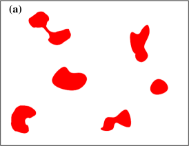
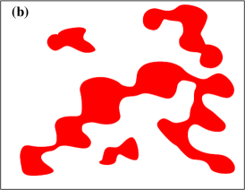
Figure 1: The examples of localized (a), delocalized (b), and inherently global (c) structure.

2 The case of well-defined support

In this section we will assume that for every typical gauge background we were given a subset ${\cal S}^{\varphi}$ of space-time $\Omega$ which dominates the behavior of some local physical quantity ${\varphi}(x)$ defined on $\Omega$. Such support ${\cal S}^{\varphi}$ could have been determined via exponential localization or by using some physical input which helped to select it uniquely for typical configurations contributing to regularized QCD path integral. It should be noted that when we talk about “space-time” we implicitly have in mind a finite hypercubic discretization of the torus with inherited Euclidean metric. However, the considerations of this section are independent of this assumption, and one can equally well think of the Euclidean torus itself. To proceed, it will be useful to first define the notion of space-time geometric structure as it will be used here and in some other studies of the subject.

2.1 Geometric structure and its global behavior

We adopt a very general definition of geometric structure which can be easily refined when used in more specific situations. It should be emphasized that the discussion in this subsection is purely geometrical and independent from the physics context in which it will be applied.

Definition ( Geometric Structure ):  Let $\Omega$ be the set of space-time points. The collection ${\rm S}=\{{\cal S}_{i},\,i=1,\ldots,N\,\}$ of path-connected subsets ${\cal S}_{i}\subset\Omega$ such that ${\cal S}_{i}\cup{\cal S}_{j}$ is disconnected for all $i\neq j$ will be referred to as a geometric space-time structure.

In case of hypercubic lattice the term path-connectivity means the usual link connectivity. The reason why the above definition focuses on path-connected sets is the underlying expectation that in physically relevant situations such sets will be associated with mediation of long-distance physics.

We wish to characterize the degree of global behavior in geometric structure S via that of its connected components ${\cal S}_{i}$. To do that, we need a notion of “linear size” for connected components regardless of their shapes. This is standard for arbitrary subsets of metric spaces and is defined as a maximum (supremum) over distances between any two points of the set.

Definition ( Linear Size ):  Let $\Gamma$ be the subset of the Euclidean space-time $\Omega$. The linear size of $\Gamma$ is defined as ${\ell}(\Gamma)\equiv\max\{\,|x-y|:\;x,y\in\Gamma\,\}$.

The subset $\Gamma$ of space-time will be called global if its linear size is comparable to the size of the underlying space, i.e. ${\ell}(\Gamma)\approx{\ell}(\Omega)$. Conversely, $\Gamma$ will be called localized if ${\ell}(\Gamma)\ll{\ell}(\Omega)$.

To quantify the degree of global behavior in geometric structure S, it is useful to define the following two characteristics. The first is the maximal linear size ${\ell}_{max}({\rm S})$ of the connected component, i.e.

$${\ell}_{max}({\rm S})\;\equiv\;\max_{{\cal S}_{i}\in{\rm S}}\,\{\,{\ell}({\cal S}_{i})\,\}$$ (1)

The second is the point-wise average of the linear size over the points of the structure. More precisely, to every point $x\in{\cal S}\equiv\cup_{i}{\cal S}_{i}$ we assign the linear size of the corresponding connected component, and take the average over ${\cal S}$

$${\ell}_{\rm S}(x)\;\equiv\;{\ell}({\cal S}_{i}),\;x\in{\cal S}_{i}\qquad\qquad{\ell}_{pta}({\rm S})\,\equiv\,\langle\,{\ell}_{\rm S}(x)\,\rangle_{{\cal S}}$$ (2)

Note that ${\ell}_{\rm S}(x)$ is a piece-wise constant function on ${\cal S}$. For continuum space-time manifold $\Omega$ a precise definition of the integrals entering the mean value has to be given for different classes of subsets ${\cal S}_{i}$. However, for the regularized case of discretized torus the above expression has the usual meaning of the point-wise average.

The purpose of introducing ${\ell}_{max}({\rm S})$ and ${\ell}_{pta}({\rm S})$ is that their values can signal different regimes of global behavior in the structure. Indeed, while ${\ell}_{max}({\rm S})$ indicates whether there is any global behavior within the structure at all, ${\ell}_{pta}({\rm S})$ measures to what extent is such behavior prevalent in the structure as a whole. Obviously, ${\ell}_{pta}({\rm S})\leq{\ell}_{max}({\rm S})$ for arbitrary S. Let us distinguish three typical situations:

(a) ${\ell}_{pta}({\rm S})\leq{\ell}_{max}({\rm S})\ll{\ell}(\Omega)\;$ (localized structure).   In this case all connected components behave as localized subsets. Fig. 1a represents an example of such geometric behavior.

(b) ${\ell}_{pta}({\rm S})<{\ell}_{max}({\rm S})\approx{\ell}(\Omega)\;$ (partially global structure). Here only parts of the structure behave as strictly global, while parts of it can still have localized character. Fig. 1b illustrates this case.

(c) ${\ell}_{pta}({\rm S})\approx{\ell}_{max}({\rm S})\approx{\ell}(\Omega)\;$ (global structure). In this case the structure has to be viewed as global since it is completely dominated by global connected parts, as exemplified in Fig. 1c.

In essence, we are proposing to associate with any geometric structure two non-negative numbers less than one, namely ${\ell}_{pta}({\rm S})/{\ell}(\Omega)$ and ${\ell}_{max}({\rm S})/{\ell}(\Omega)$. These values quantify the global behavior of the structure. We emphasize that the above classification is purely geometrical and will be useful only to the extent to which the characteristic situations described above turn out to be typical for space-time structures occurring in the QCD vacuum.

2.2 Support from physics considerations

We now come back to the discussion of the situation where the space-time support ${\cal S}^{\varphi}\subset\Omega$ corresponding to local observable ${\varphi}(x)$ is assumed to be uniquely determined on physical grounds. It is easy to see that ${\cal S}^{\varphi}$ defines a space-time structure S^φ as defined in the previous subsection. Indeed, arbitrary ${\cal S}^{\varphi}$ can be uniquely decomposed into maximal connected subsets, i.e. ${\cal S}^{\varphi}=\cup_{i}{\cal S}^{\varphi}_{i}$ such that ${\cal S}^{\varphi}_{i}$ is connected, and that ${\cal S}^{\varphi}_{i}\cup{\cal S}^{\varphi}_{j}$ is disconnected for all $i\neq j$. Then S${}^{\varphi}=\{{\cal S}_{i}^{\varphi},\,i=1,\ldots,N\,\}$. We can thus use the geometric concepts of the previous subsection to characterize the degree of its global behavior. However, since the geometry of S^φ has been determined by the underlying physics, the global or localized geometric nature of S^φ are expected to be manifestations of qualitatively very different types of underlying dynamics which we try to understand. We are implicitly making the following associations:

(a) If S^φ behaves as localized geometric structure, then we expect the vacuum objects driving the dynamics of the gauge field also to be localized, with typical size approximately given by ${\ell}_{pta}({\rm S}^{\varphi})$. From the physics point of view we are thus dealing with localized structure.

(b) If S^φ behaves as partially global geometric structure, it is an indication that we are dealing with delocalized physical structure. Indeed, the presence of global connected subsets signals that the dynamics produces correlations over very large distances but, at the same time, the presence of localized subsets points to the existence of underlying localized objects that mediate this correlation. Such objects can still serve as a useful tool for theoretical analysis of the situation.

(c) If S^φ behaves as global geometric structure, then this indicates that the underlying dynamics produces correlations that universally span the whole system. This could happen as a result of two qualitatively different physical situations. The first is the case of extreme delocalization, wherein the underlying localized objects are essentially never seen individually, but can still be distinguished within the global subsets and are relevant for physics. The second possibility is that the global subsets do not contain any privileged parts and behave as a single whole. Here the notion of a localized object is no longer useful to analyze the physics, and the structure is inherently global (super-long-distance).

To avoid the confusion in nomenclature in what follows, let us summarize. Our goal is to be able to distinguish three physically distinct situations: localized, delocalized and inherently global (super-long-distance) behavior. At the same time, we introduced the concepts that distinguish three geometric space-time arrangements: geometrically localized, partially global and global structure. If there is a well-defined support ${\cal S}^{\varphi}$ dominating the physical behavior of ${\varphi}$, we associate the localized geometric nature of corresponding S^φ with the underlying localized physical behavior. Similarly, the partially global nature of S^φ is associated with delocalization. However, if ${\cal S}^{\varphi}$ is a global geometric structure, we could be dealing with two qualitatively different physical cases, namely extreme delocalization or super-long-distance behavior. To distinguish the two, one could introduce additional geometric concepts. However, we will take a different approach in what follows.

3 The use of fraction supports

While the discussion of the previous section provides a partial basis for analyzing the issues of localization, it is not quite satisfactory. Indeed, the main problem is that frequently it is not possible to use it because there is no unique way to determine the support for given local quantity ${\varphi}(x)$ from physics considerations or otherwise. Even though there are many ways to assign a support to a function in a generic way (i.e. regardless of the functional form), the arbitrariness of such procedures makes it dangerous for making definite conclusions. We discuss the related issues in the Appendix A.

In order to overcome this shortcoming, we propose to work with many “potential” supports and monitor both the degree of global behavior, and the degree to which ${\varphi}(x)$ is concentrated in such possible supports. In this way, much more complete information enters the consideration. We will argue and demonstrate (both here and in upcoming publications) that this strategy leads to definite conclusions in the specific case of QCD vacuum structure. The procedure can be described in few steps and, to exemplify the discussion, we will frequently refer to the case of Schrödinger wave function, i.e. ${\varphi}(x)\longrightarrow\psi(x)$, where $x$ is a space coordinate. In what follows, we will assume (both in definitions and formulas) that $\Omega$ is a hypercubic discretization of the torus.

1. Choose a positive semi-definite measure ${\mu}^{\varphi}(x)$ that characterizes the physically relevant “strength” (intensity) of ${\varphi}(x)$. For Schrödinger wave function this is obviously ${\mu}^{\psi}(x)=\psi^{\dagger}(x)\psi(x)$ because this represents the probability density for the particle to be in the vicinity of $x$. The role of ${\mu}^{\varphi}(x)$ is to introduce an importance ranking for all space-time points: high-intensity points are physically more relevant than low-intensity points. This allows us to define the family of nested subsets ${\cal S}^{\varphi}(f)$ (fraction supports) respecting this ranking.

Definition (Fraction Support):  Let ${\varphi}(x)$ be the local observable on space-time $\Omega$ with intensity ${\mu}^{\varphi}(x)$. The collection ${\cal S}^{\varphi}(f)\subset\Omega$ of highest intensity-ranked space-time points that occupy fraction $f$ of available volume, i.e. $N({\cal S}^{\varphi}(f))/N(\Omega)=f$, will be referred to as a fraction support corresponding to $f$ and ${\varphi}(x)$.

In the above definition the “volume” $N(\Gamma)$ for arbitrary $\Gamma\subset\Omega$ represents the number of lattice points contained in $\Gamma$. The sets ${\cal S}^{\varphi}(f)$ form a family of potential supports whose global behavior will be examined.

2. While the volume fraction $f$ is a convenient label for fraction supports, we also need a measure expressing how good a support ${\cal S}^{\varphi}(f)$ would be, i.e. to which degree the behavior of ${\varphi}(x)$ within ${\cal S}^{\varphi}(f)$ dominates relative to the whole $\Omega$. In case of Schrödinger particle the appropriate measure is the total probability of the particle to be within the support, i.e. the sum of ${\mu}^{\psi}(x)=\psi^{\dagger}(x)\psi(x)$ over ${\cal S}^{\psi}(f)$. In general, this information is contained in the normalized cumulative function of intensity

$${\cal C}^{\varphi}(f)\,\equiv\,{\;\sum\limits_{{\cal S}^{\varphi}(f)}\,{\mu}^{\varphi}(x)\;}/{\;\sum\limits_{\Omega}\,{\mu}^{\varphi}(x)\;}$$ (3)

At the regularized level considered here (before taking the continuum limit) $f$ is a discrete variable chosen from the set $\{\,n/N(\Omega),\,n=0,1,2,\ldots,N(\Omega)\,\}\subset[0,1]$. However, we will keep the “continuous” notation and associate ${\cal C}^{\varphi}(f)$ with a continuous piece-wise linear function connecting the points of the discrete map. In the continuum limit (and as a regularized approximation), ${\cal C}^{\varphi}(f)$ is a non-decreasing concave function from interval $[0,1]$ to itself, such that ${\cal C}^{\varphi}(1)=1$. If ${\mu}^{\varphi}(x)$ is non-zero only in a single point or on the set of measure zero, then ${\cal C}^{\varphi}(f)=1$ identically. In the other extreme situation when ${\mu}^{\varphi}(x)$ is constant through space-time, we have ${\cal C}^{\varphi}(f)=f$. In case of arbitrary strict support, i.e. when there exists $\Gamma\subset\Omega$ such that ${\mu}^{\varphi}(x)\neq 0$ for $x\in\Gamma$ and ${\mu}^{\varphi}(x)=0$ for $x\not\in\Gamma$, the function ${\cal C}^{\varphi}(f)$ reaches value $1$ at the corresponding fraction $f_{\Gamma}$ and remains constant on the interval $[f_{\Gamma},1]$.

We emphasize that ${\cal C}^{\varphi}(f)$ is a basic characteristic of the space-time structure induced by ${\varphi}(x)$. It has a specific behavior for particular classes of space-time distributions and contains detailed quantitative information about how much is ${\varphi}(x)$ concentrated in fraction supports ${\cal S}^{\varphi}(f)$. We propose that this information is necessary in order to judge the potential global character of the physically relevant structure.

3. Every fraction support ${\cal S}^{\varphi}(f)$ generates a corresponding geometric structure S${}^{\varphi}(f)$ via decomposition into maximal connected subsets. To monitor the global behavior of these structures, we compute the corresponding characteristics introduced in Sec. 2.1, and thus define the functions

$${\ell}_{max}^{\varphi}(f)\equiv{\ell}_{max}({\rm S}^{\varphi}(f))\qquad\qquad{\ell}_{pta}^{\varphi}(f)\equiv{\ell}_{pta}({\rm S}^{\varphi}(f))$$ (4)

When measuring the length in the units of maximal linear distance ${\ell}(\Omega)$ (which we will assume from now on), then ${\ell}_{max}^{\varphi}(f)$ and ${\ell}_{pta}^{\varphi}(f)$ are functions from interval $[0,1]$ to itself and ${\ell}_{max}^{\varphi}(1)={\ell}_{pta}^{\varphi}(1)=1$ similarly to ${\cal C}^{\varphi}(f)$ (see however Sec. 3.1). Contrary to ${\cal C}^{\varphi}(f)$ though, these functions are not necessarily concave. Also, ${\ell}_{max}(f)$ is a non-decreasing function, while the monotonic properties of ${\ell}_{pta}(f)$ are indefinite in general.

We have thus defined three characteristic functions associated with local physical observable ${\varphi}(x)$ defined on space-time $\Omega$. While ${\cal C}^{\varphi}(f)$ describes and quantifies the tendency of ${\varphi}(x)$ to be concentrated in preferred regions of space-time, ${\ell}_{max}^{\varphi}(f)$ and ${\ell}_{pta}^{\varphi}(f)$ describe and quantify the degree of global behavior for such preferred regions. The knowledge of these functions allows us to judge the degree of global behavior for arbitrary degree of saturation in physically relevant intensity ${\mu}^{\varphi}(x)$. We propose that this detailed information has to be considered in conjunction in order to make definite conclusions on whether the physical structure inducing the behavior of ${\varphi}(x)$ is localized, delocalized, inherently global or indefinite. Following the discussion in Sec. 2, we distinguish three typical and qualitatively different types of behavior shown schematically in Fig. 2.

(i)

${\cal C}^{\varphi}(f)$ saturates considerably faster than ${\ell}_{max}^{\varphi}(f)$ as exemplified in Fig. 2a. This means that at fractions where ${\cal C}^{\varphi}(f)$ starts to saturate (smallest fractions such that ${\cal C}^{\varphi}(f)\>\raisebox{-3.44444pt}{$\stackrel{{\scriptstyle\raisebox{-4.52083pt}{$\textstyle<$}}}{{\sim}}$}\>1$) the corresponding fraction supports form a localized geometric structure, i.e. ${\ell}_{max}^{\varphi}(f)\ll{\cal C}^{\varphi}(f)$. In this case we classify the underlying physical structure as localized since the dominating fields are concentrated on such geometric structure.

(ii)

${\cal C}^{\varphi}(f)$ saturates at similar fractions as either ${\ell}_{max}^{\varphi}(f)$ or ${\ell}_{pta}^{\varphi}(f)$, or in between the two, as exemplified in Fig. 2b. This situation indicates that the underlying physical structure is delocalized. Indeed, if ${\cal C}^{\varphi}(f)$ saturates faster than ${\ell}_{pta}^{\varphi}(f)$ then the fraction support at the point of saturation forms a partially global geometric set, i.e. ${\ell}_{max}^{\varphi}(f)\approx{\cal C}^{\varphi}(f)>{\ell}_{pta}^{\varphi}(f)$, which is typical of delocalization (see Sec. 2.2). On the other hand, if ${\cal C}^{\varphi}(f)$ and ${\ell}_{pta}^{\varphi}(f)$ saturate at approximately the same rate, then we are dealing with geometrically global structure at the point of saturation, which is common both to extremely delocalized and inherently global cases. However, the signature of extremely delocalized structure is that a small decrease in fraction changes global geometric behavior to partially global, where some individual localized objects starts to appear in isolation. This is precisely what happens in this case.

(iii)

${\cal C}^{\varphi}(f)$ saturates considerably slower than ${\ell}_{pta}^{\varphi}(f)$, as shown in Fig. 2c. This means that at fractions where ${\cal C}^{\varphi}(f)$ starts to saturate the corresponding fraction supports form a geometrically global structure, i.e. ${\ell}_{pta}^{\varphi}(f)\approx{\cal C}^{\varphi}(f)$. Moreover, this arrangement is very stable with respect to the change of the fraction. This indicates that the underlying physical structure is inherently global (super-long-distance).

We emphasize that a generic space-time arrangement does not necessarily have to fall into any of the typical cases described above. If that happens, than we have an indefinite situation which has to be analyzed in more detail by other means.

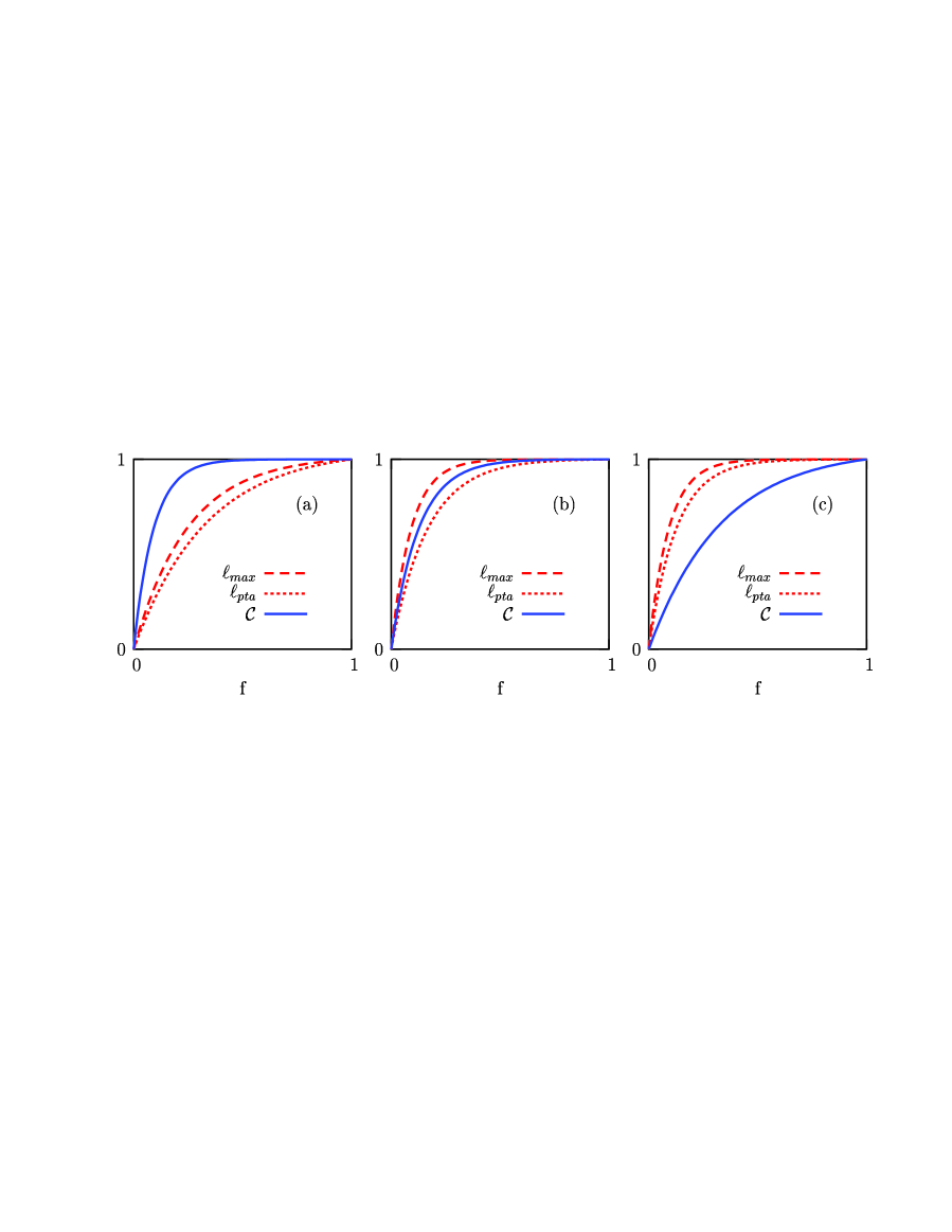
Figure 2: The signatures of localized (a), delocalized (b), and inherently global (c) behavior.

4. While the fraction $f$ of space-time is a convenient variable to introduce the functions ${\cal C}^{\varphi}(f)$, ${\ell}_{max}^{\varphi}(f)$ and ${\ell}_{pta}^{\varphi}(f)$, there is a more economic way to convey the physics information on global behavior. Indeed, the above characteristics provide answer to the following relevant question. Given arbitrary degree of saturation ${\cal C}^{\varphi}$ ($0\leq{\cal C}^{\varphi}\leq 1$), what are the values of ${\ell}_{max}^{\varphi}$, ${\ell}_{pta}^{\varphi}$ characterizing the global behavior of the corresponding fraction support where fields are concentrated? In case of a Schrödinger wave function we could ask what are the global characteristics of the minimal region of space comprising e.g. $90$% chance to find the particle. We can express this information directly by eliminating $f$ in favor of ${\cal C}^{\varphi}$. In generic case this can be done since $f\mapsto{\cal C}^{\varphi}(f)$ is a one-to-one map of the interval $[0,1]$ to itself. Formally, we are introducing the change of variable

$${\ell}_{max}^{\varphi}(f)\;\longrightarrow\;{\ell}_{max}^{\varphi}(f({\cal C}^{\varphi}))\qquad\quad{\ell}_{pta}^{\varphi}(f)\;\longrightarrow\;{\ell}_{pta}^{\varphi}(f({\cal C}^{\varphi}))$$ (5)

While the functional forms are obviously different after the change of variable, we will keep the same notation, namely ${\ell}_{max}^{\varphi}({\cal C})$ and ${\ell}_{pta}^{\varphi}({\cal C})$, where it is implicitly assumed that ${\cal C}$ is related to local field ${\varphi}(x)$. We also note that for many relevant questions ${\cal C}$ is indeed a more physical variable in the sense that ${\cal C}$ (rather than $f$) should be fixed when approaching a continuum limit.

It is straightforward to see how the typical localized, delocalized and global physical behavior reflects in the functions ${\ell}_{max}^{\varphi}({\cal C})$ and ${\ell}_{pta}^{\varphi}({\cal C})$. In Fig. 3 we plot these functions corresponding to cases shown in Fig. 2.

Figure 3: The signatures of localized (a), delocalized (b), and inherently global (c) behavior.

3.1 Partitioning of the fraction support

In our discussion so far, the space-time structure was introduced solely via the behavior of ${\mu}^{\varphi}(f)$, and the resulting geometric properties of fraction supports. However, there could be additional physics aspects of local observable ${\varphi}(x)$, which should be taken into account when judging the global properties. A typical example is represented by topological charge density $q(x)$, whose sign has important physical consequences. Indeed, the quarks of preferential chirality are attracted to regions of definite sign. This is expected to be very relevant for understanding various aspects of hadron structure and hadron propagation. In such a case it is then appropriate to partition the fraction support accordingly, and to consider global properties of the physically relevant partitioned sets [1, 2, 5]. In general case, we will thus consider the sets ${\cal S}^{\varphi}_{r}(f)$, $r=1,\ldots,R$, such that $\cup_{r}{\cal S}^{\varphi}_{r}(f)={\cal S}^{\varphi}(f)$, and ${\cal S}^{\varphi}_{r}(f)\cap{\cal S}^{\varphi}_{s}(f)=\emptyset$ for all $r$, $s$. There are several things that should be pointed out with regard to this situation.

(1) The cumulative function ${\cal C}^{\varphi}(f)$ is not affected by partitioning and is defined in the usual way relative to ${\cal S}^{\varphi}(f)$.

(2) The global characteristics ${\ell}_{max}^{{\varphi},r}(f)$, ${\ell}_{pta}^{{\varphi},r}(f)$ will characterize the partitioned sets and the only generic property that will change in this regard is that they do not necessarily approach unity as $f\rightarrow 1$. In principle then the values ${\ell}_{max}^{{\varphi},r}(1)$ and ${\ell}_{pta}^{{\varphi},r}(1)$ are relevant characteristics that enter the classification of global properties. It is straightforward to extend our discussion to include them.

(3) If there is a symmetry in the theory which relates the average properties of partitioned fraction supports (which is usually the case), then the global characteristics for different $r$ just represent samples (possibly correlated) for the unique functions ${\ell}_{max}^{\varphi}(f)$ and ${\ell}_{pta}^{\varphi}(f)$.

3.2 Loose ends

Our discussion in the main part of this section concentrated on clear exposition of basic ideas in our approach, but left open certain issues that arise in special cases. In what follows we will consider some of them.

The first is the definition of the fraction support (at the regularized level) if some functional values of ${\mu}^{\varphi}(x)$ are degenerate. The extreme case is that of a constant field ${\varphi}(x)$. The problem is how to assign the ranking within the degenerate subset, so that the associated fraction supports lead to unique definition of ${\cal C}^{\varphi}(f)$, ${\ell}_{pta}^{\varphi}(f)$ and ${\ell}_{max}^{\varphi}(f)$. Note that this is not a problem for definition of ${\cal C}^{\varphi}(f)$ and arbitrary ad hoc rule leads to the same function. However, the functions ${\ell}_{pta}^{\varphi}(f)$ and ${\ell}_{max}^{\varphi}(f)$ can in principle depend on the rule chosen. It is straightforward to complete the definition of these functions in arbitrary degenerate case, so that the notion of localization, delocalization and global behavior (as defined here) will correspond to its intended meaning. To do that, note that the process of ranking the space-time points corresponds to specifying a non-repeating sequence $x_{1},x_{2},\ldots,x_{N(\Omega)}$. Denoting the sets of points contained in partial sequences containing $n$ points as ${\cal P}^{n}=\{x_{1},x_{2},\ldots,x_{n}\}$, assume that this partial sequence has been assembled. Then the rules for continuing the sequence recursively are the following: (1) If the next value of intensity, i.e. ${\mu}^{\max}_{n}\equiv\max\{\,{\mu}^{\varphi}(x),x\in\Omega-{\cal P}^{n}\,\}$ is non-degenerate, then $x_{n+1}=y$ such that ${\mu}^{\varphi}(y)=\mu^{\max}_{n}$. (2) If $\mu^{\max}_{n}$ is $k$-fold degenerate, i.e. if there are points $y_{1},y_{2},\ldots,y_{k}$ such that ${\mu}^{\max}_{n}={\mu}^{\varphi}(y_{1})=\ldots={\mu}^{\varphi}(y_{k})$, then we need to specify the permutation $p(i),i=1,\ldots,k$ such that $x_{n+i}=y_{p(i)}$. We require this permutation to be chosen in such a way that ${\ell}_{max}^{\varphi}(f)$ grows fastest for arguments $f_{m}\equiv m/N(\Omega),\,m\in\{n+1,n+2,\ldots,n+k\}$. More precisely, we require that (i) ${\ell}_{max}^{\varphi}(f_{n+1})-{\ell}_{max}^{\varphi}(f_{n})$ is maximal over all permutations. (ii) If this does not specify permutation $p$ uniquely, we consider the restricted degenerate set of permutations and further require that ${\ell}_{max}^{\varphi}(f_{n+2})-{\ell}_{max}^{\varphi}(f_{n+1})$ is maximal. (iii) This recursion continues and stops when $p$ is uniquely determined. (iv) If $p$ is not uniquely determined at the end of the finite recursion, we choose it from the remaining degenerate set by arbitrary fixed rule. One can easily check that the resulting ${\ell}_{max}^{\varphi}(f)$ and ${\ell}_{pta}^{\varphi}(f)$ are invariant under this remaining freedom. Note also that the above rules lead to classification of the constant field ${\varphi}(x)$ as global configuration which is appropriate.

The second class of situations which needs to be mentioned is exemplified by the following. Assume the existence of a strict support which becomes the set of measure zero in the continuum limit. For example, a strict support could form form a finite low-dimensional manifold. In that case ${\cal C}^{\varphi}(f)\equiv 1$ in the continuum limit, and thus ${\cal C}^{\varphi}(f)$ will not carry any information about the behavior within the support. In that case one has to define the cumulative function and the corresponding global characteristics for the support itself. In the other extreme case the global characteristics ${\ell}_{max}^{\varphi}(f)$ or ${\ell}_{pta}^{\varphi}(f)$ could become identically one in the continuum limit, indicating a global behavior on sets of lower dimension. These situations are of particular interest for QCD vacuum case [2], and will be addressed in a separate publication.

4 Cases of physical interest

In this section we will discuss in more detail few basic examples of local observables ${\varphi}(x)$ which are of interest for studies of QCD vacuum structure, and which will be analyzed in the upcoming publications. In particular, we will mention observables related to gauge fields $U_{\mu}(x)$ and the Dirac eigenmodes $\psi_{\lambda}(x)$. To ease the notation, from now on we will skip labels of ${\varphi}(x)$ on various characteristics discussed. The appropriate association will be obvious from the context. In this section we will also give examples (in case of Dirac eigenmodes) of how the methods developed here work in QCD.

4.1 Gauge fields

In pure glue lattice gauge theory all local observables are constructed from fundamental gauge fields $U_{\mu}(x)\equiv e^{igA_{\mu}(x)}$. The intensity of gauge fields is physically associated with the corresponding field-strength tensor $U_{\mu}(x)\rightarrow F_{\mu\nu}(x)$ describing chromo-electric and chromo-magnetic fields. Two basic physically relevant composite fields characterizing the intensity of $F_{\mu\nu}$ are the scalar density $s(x)\propto{\tt tr}F_{\mu\nu}F_{\mu\nu}(x)$ (action density) and the pseudoscalar density $q(x)\propto{\tt tr}F_{\mu\nu}\tilde{F}_{\mu\nu}(x)$ (topological density). Understanding the space-time structure of $s(x)$ and $q(x)$ in configurations dominating the QCD path integral is one of the most basic ingredients for understanding the QCD vacuum structure.

To characterize the global properties of this structure according to the scheme developed in previous sections, we first have to specify the corresponding physically relevant intensities. Since $s(x)$ is positive semidefinite, it can serve as its own intensity ${\mu}(x)$. One might be tempted to consider other positive-semidefinite functions of $s(x)$, e.g. the powers $\mu(x)=s^{\alpha}(x)$ for $\alpha>0$. The cumulative functions ${\cal C}(f)$ would obviously be different for different values of $\alpha$. However, while the intensity corresponding to $\alpha=1$ has a well-defined physical meaning (we study the space-time distribution of the action), this is not so for other values of $\alpha$. Similarly, for $q(x)$ the appropriate intensity to use is ${\mu}(x)\equiv|q(x)|$, since it allows for relevant comparison to the behavior of $s(x)$.

In the case of $q(x)$ there is a more physically-motivated approach suggested by the fact that global fluctuations of topological charge are directly related to the $\eta^{\prime}$ mass via Witten–Veneziano relation [12]. One would thus like to judge the global properties of the relevant space-time structure relative to the saturation of topological susceptibility. While conceptually this conforms to the general strategy developed here, it requires some technical modifications which we now describe.

The main change one has to deal with is the definition of the cumulative function ${\cal C}(f)$ because there is no intensity ${\mu}(x)$, local in the gauge fields, that one could use to define this function directly using Eq. (3). Nevertheless, assuming that a well-defined topological density operator (such as the operator associated with Ginsparg-Wilson fermions [13, 14]) is at our disposal, it is still possible to construct the appropriate cumulative function which will play the corresponding role in classifying the global behavior of the space-time structure. Indeed, defining the fraction supports ${\cal S}(f)$ relative to ${\mu}(x)=|q(x)|$, let us consider the corresponding cumulative charge $Q(f)$, and the associated fluctuation $\chi(f)$ which is only defined in the ensemble average

$$\chi(f)\,\equiv\,\frac{\langle\,Q^{2}(f)\,\rangle\,-\,\langle\,Q(f)\,\rangle^{2}}{V}\qquad\qquad Q(f)\,\equiv\,\sum_{x\in{\cal S}(f)}q(x)\qquad\quad$$ (6)

where $V=a^{4}N(\Omega)$ is the physical volume. We then define the normalized cumulative function of global fluctuations via

$${\cal C}(f)\;\equiv\;\chi(f)/\chi(1)$$ (7)

There are two points that need to be emphasized here. (1) While we call the ${\cal C}(f)$ defined above a cumulative function in analogy with definition in Eq. (3), it is not a priori obvious that it has the specific properties of the cumulative function. In particular, it is not obvious that it is a concave non-decreasing function. Indeed, we are making an assumption that the ordering induced by $|q(x)|$ will ensure these properties in the ensemble average. This is reasonable since it is expected that regions with most intense fields will contribute most to global fluctuations. Our numerical data a posteriori confirm that this is indeed the case in QCD [15]. (2) The precise determination of ${\cal C}(f)$ does not necessarily require the use of very large ensembles to compute the physical susceptibility $\chi(1)$ to comparable accuracy. Indeed, computing ${\cal C}(f)$ directly via jackknife samples of $\chi(f)/\chi(1)$ leads to much smaller fluctuations over the whole range of $f$ [15].

4.2 QCD Dirac Zero Modes

For Dirac eigenmodes $\psi_{\lambda}(x)$ ( i.e. $D\psi_{\lambda}(x)=\lambda\psi_{\lambda}(x)$ ) the basic scalar and pseudoscalar composites are the “density” $d_{\lambda}(x)\equiv\psi_{\lambda}^{\dagger}(x)\psi_{\lambda}(x)$ and “chirality” $c_{\lambda}(x)\equiv\psi_{\lambda}^{\dagger}(x)\gamma_{5}\psi_{\lambda}(x)$. However, the zero modes are globally chiral and this is exactly true even on the lattice if overlap fermions are used (which we assume). We thus only have one independent bilinear to study, which we choose to be the density ${\varphi}(x)\equiv d(x)$. In direct analogy to the case of Schrödinger particle, the associated intensity ${\mu}(x)$ for determining the fraction supports and for computing the cumulative functions will be the density $d(x)$ itself. Note that the choice of the bilinear form (rather than higher powers) is further physically motivated by the fact that the fermionic action is bilinear in fermion fields.

To illustrate how the global characteristics of the space-time structure introduced here behave in QCD, we have analyzed the low-lying eigenmodes of the overlap operator. In particular, we have considered an ensemble of $20$ Wilson gauge configurations on $16^{4}$ lattice at $\beta=6.07$. This corresponds to the lattice spacing of $a=0.082$ fm as determined from the string tension [16], and the linear extent $L\approx 1.3$ fm. The eigenmodes of the overlap operator with negative mass $\rho=1.368$ ($\kappa=0.19$) were computed using the Zolotarev approximation to implement the operator numerically. The details of this numerical implementation are given elsewhere (see e.g. [1, 17]).

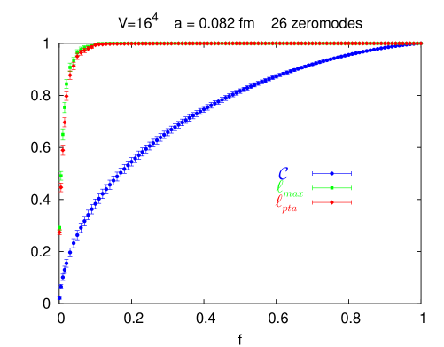
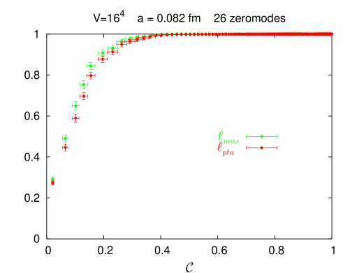
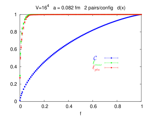
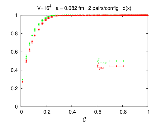
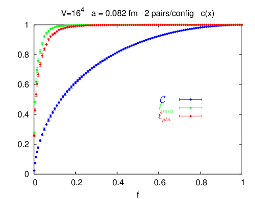
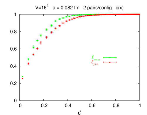
Figure 4: Characteristics of global behavior for Dirac zero modes (top), Dirac near-zero modes via density (middle) and Dirac near-zero modes via chirality (bottom). The structure is clearly super-long-distance in all cases. See the discussion in the text.

We found the total of $26$ zero modes in the above ensemble and computed the average ${\cal C}(f)$, ${\ell}_{max}(f)$ and ${\ell}_{pta}(f)$. The results are shown in Fig. 4 (top left) together with the associated ${\ell}_{max}({\cal C})$ and ${\ell}_{pta}({\cal C})$ (top right). One can clearly observe that the structure is geometrically global at the fractions of just few percent (e.g. ${\ell}_{pta}(f=0.036)=0.9$ ). At such fractions the cumulative function only achieves values ${\cal C}\approx 0.2$. Following our discussion in Sec. 3 we thus conclude that we clearly observe a super-long-distance space-time structure in QCD Dirac zero modes. Note also that ${\ell}_{max}(f)$ and ${\ell}_{pta}(f)$ are quite close to one another, indicating that there is very little fragmentation at arbitrary fraction. In fact, the structure typically comes in a single dominating piece as it is grown from very small fractions up.

4.3 QCD Dirac Near-Zero Modes

In the case of near-zero modes we can study the global behavior in both $d(x)$ and $c(x)$. Due to $\gamma_{5}$-Hermiticity, the near-zero modes of the overlap operator come in complex-conjugate pairs with identical $d(x)$ and $c(x)$. We will thus consider only a single representative of the pair. For our calculation, we have considered two lowest-lying pairs for every configuration from the ensemble. This gave us altogether $40$ modes to analyze.

We start with the density for which the appropriate intensity is ${\mu}(x)\equiv d(x)$ as in the case of zero modes. The resulting global characteristics are shown in Fig. 4 (middle). From this data it is very clear again that the scalar structure in QCD near-zero modes is super-long-distance. For example, ${\ell}_{pta}(f=0.038)=0.9$, while ${\cal C}\approx 0.16$ at the same fraction. Similarly to zero modes, the functions ${\ell}_{max}(f)$ and ${\ell}_{pta}(f)$ are quite close one to another and the structure is dominated by a single connected piece. As a side remark, note also that the cumulative function ${\cal C}(f)$ has steeper behavior in case of zero modes than in case of near-zero modes. This results in steeper behavior of functions ${\ell}_{max}({\cal C})$, ${\ell}_{pta}({\cal C})$ for near-zero modes. We will study such details in a dedicated publication [11].

In case of chirality the appropriate intensity to study is ${\mu}(x)=|c(x)|$. Since the sign of local chirality carries a relevant physical information (e.g. on the preferred duality of the underlying gauge field and the qualitative features of the quark propagation), we partition the fraction supports into subsets of definite sign (see Sec. 3.1). Since QCD dynamics has no preference for a particular chirality, we average over connected subsets of both signs in calculation of ${\ell}_{pta}(f)$. Also, in calculation of ${\ell}_{max}(f)$ we consider the maximum over connected subsets of both signs. The results are shown in Fig. 4. Again, we find the space-time characteristics corresponding to clear super-long distance structure in $c(x)$. Note that the functions ${\ell}_{pta}(f)$, ${\ell}_{max}(f)$ saturate slightly slower than in the case of $d(x)$ which is due to the partition and the fact that the connected subsets of opposite chirality “obstruct” one another in their global behavior. At the same time the cumulative function is steeper than in the case of $d(x)$ (it is in fact similar to cumulative function for zero modes) resulting in the slower saturation of ${\ell}_{max}({\cal C})$ and ${\ell}_{pta}({\cal C})$.

5 Conclusions

In this paper we have proposed the framework for studying the issues of localization in QCD vacuum in a model-independent manner . This framework was set up in such a way as to inquire into three hypothetical scenarios underlying the QCD dynamics. The first scenario (localization) involves the existence of fundamental localized objects in the gauge field populating the QCD vacuum and driving the dynamics. The second scenario (delocalization) involves localized entities which however clump into global structures (via interaction) and can support physical correlations over very large distances. A distinctive property of delocalization is that the localized objects still preserve their identity and can serve as a basis for physical analysis of vacuum properties. The third scenario (inherently global or super-long-distance behavior) is qualitatively different in that there are fundamental entities that themselves exhibit global behavior. The geometric structure of these entities can facilitate correlations over arbitrarily large distances and the vacuum properties can be fully understood only in terms of these global objects.

The approach proposed in this work is based on the idea that the existence of gauge field objects with above properties will lead to a corresponding geometric behavior in local composite fields, and possibly also in Dirac eigenmodes. In particular, the space-time regions containing dominating fields (the “support” of the field) will behave in the specific geometric manner, forming localized, partially localized or global geometric structure. However, since the definition of field support on physical grounds is not generically available, we proposed the use of cumulative functions with simultaneous monitoring of both the degree of saturation of the field, and of the global characteristics of the underlying fraction supports. It was then proposed that the specific functional behavior of these dependencies can be associated with the three physical situations described above.

We have discussed in detail the application of these ideas to special cases of action density, topological density, and to the scalar and pseudoscalar density of Dirac low-lying modes. Our approach was illustrated via the study of overlap zero modes and near-zero modes. The results clearly demonstrate the super-long distance nature of the underlying gauge structure as reflected in the Dirac eigenmodes. They also provide the quantitative validation for the original suggestion by the Kentucky group that the Dirac near-zero modes form global structure (“ridges” rather than separate peaks) [5].

Finally, as emphasized in the introduction, the aim of this paper (first in the series) is to introduce techniques suitable for analysis of QCD space-time structure obtained in a model-independent manner. In this approach, gauge fields are not processed or altered in any way, and the structure is uncovered as it appears directly in the configurations dominating the QCD path integral. The culmination of these attempts so far is the discovery of the strictly low-dimensional, inherently global sheet/skeleton structure in the overlap topological charge density [2]. The methods developed in this work (see Sec. 4.1) provide a formal framework for a detailed quantitative confirmation of the super-long-distance nature of this structure [15].

Acknowledgments

Numerous discussions with members of the Kentucky group on the topics of this work are gratefully acknowledged. Thanks to Andrei Alexandru and Hank Thacker for feedback on the manuscript. The author is indebted to Andrei Alexandru and Nilmani Mathur for help with the figures, and to Jianbo Zhang for the help with the data, part of which was used to illustrate the methods proposed in this manuscript. The Kentucky group is acknowledged for making this data available. The author benefited from communications with Ganpathy Murthy, Štefan Olejník and Joe Straley.

Appendix A Generic Definitions of the Support

Assume that we are given a generic function ${\varphi}(x)$ on space-time, and the associated real-valued positive-semidefinite intensity ${\mu}(x)$. If the specific properties of ${\varphi}(x)$ are not known, it is tempting to use some generic way of determining the space-time region where the function is effectively concentrated, i.e. its effective support. This support is implicitly associated with space-time regions occupied by strongest fields, such that fields in the rest of the space-time can either be neglected or behave in a qualitatively different (low intensity) manner. Thus, from the geometric point of view, effective support is one of the fraction supports defined in Sec. 3, and the goal of a given generic procedure is to fix the corresponding fraction (effective fraction $f_{eff}$). However, as emphasized in Sec. 3, the generic definitions of this type are highly ambiguous.

To illustrate this, let us concentrate on the scalar structure of Dirac eigenmodes. The same discussion can be extended straightforwardly to the case of arbitrary local observable ${\varphi}(x)$. Given a (normalized) Dirac eigenmode $\psi(x)$, the physically relevant intensity characterizing its (scalar) strength is ${\mu}(x)\equiv d(x)=\psi^{\dagger}\psi(x)$, and the definition of the support will thus be given in terms of this associated function $f_{eff}=f_{eff}[d(x)]$. Consider, for example, the following definitions of $f_{eff}$.

(1) A natural possibility is to base the definition on the behavior of the corresponding cumulative function ${\cal C}(f)$. In Fig. 5 (left) we show ${\cal C}(f)$ for the zero mode #1 from the set analyzed in Sec. 4.2. Even though we work on the latticized torus with $N$ sites, we will keep the “continuous” notation and treat ${\cal C}(f)$ as a piece-wise linear continuous function connecting the points of the discrete map (see Sec. 3). ${\cal C}(f)$ is a concave function on the interval $[0,1]$ such that ${\cal C}(0)=0$ and ${\cal C}(1)=1$, and hence $1\geq I\equiv\int_{0}^{1}df\,{\cal C}(f)\geq 1/2$. Clearly, if $d(x)$ is sharply concentrated on small fraction of space-time, then $I\approx 1$, and when $d(x)$ is spread out over the whole lattice then $I\approx 1/2$. In an extreme case of localization on single site we have $I=1-1/2N$ ($I=1$ in the continuum limit), and $I=1/2$ for constant $d(x)$. We can thus in principle base the definition of $f_{eff}$ on the value of $I$. The simplest possibility is to use the linear expression in $I$ which interpolates between the above extreme values, i.e.

$$f_{eff}\,\equiv 2(1-I)\,\equiv\,f_{1}$$ (8)

This definition gives $f_{1}=1/N$ and $f_{1}=1$ for $d(x)=\delta_{x,y}$ and $d(x)=1/N$ respectively. Also, $0\leq f_{1}\leq 1$ for arbitrary $d(x)$, and thus $f_{1}$ has the intended meaning of the effective fraction. It is “tailored” for the functions $d(x)$ that are constant on fraction $f_{1}$ of sites and vanish on the rest of the sites. In effect then, the above procedure associates with arbitrary $d(x)$ a unique function of this type, such that the corresponding integrals $I$ are the same. In Fig. 5 (left) we show the value $f_{1}$ together with the cumulative function ${\cal C}_{1}$ for the associated constant function on the strict support.

(2) Other than its simplicity, there is no particular reason to choose $f_{1}$ to be the definition of effective fraction in a generic situation. For example, instead of relating $d(x)$ to the constant function on strict support, we could relate it to the function which is constant and non-zero both on the support and (with lower intensity) on the complement of the support. To uniquely specify such function (and with it the corresponding fraction $f_{eff}\equiv f_{2}$), we can e.g. require simultaneously that (a) the integrals $I$ of the cumulative functions are the same and that (b) the corresponding ${\cal C}_{2}(f)$ is the best approximation of ${\cal C}(f)$, i.e. that $\int_{0}^{1}df\,({\cal C}(f)-{\cal C}_{2}(f))^{2}$ is minimal. With this choice the resulting $f_{2}$ and ${\cal C}_{2}(f)$ for zero mode # 1 are shown in Fig 5 (left). Note that this definition could be useful if it is a priori known that the actual space-time distributions in question have a well-defined, approximately constant core, but also an approximately constant background. Again, in the extreme cases of $d(x)=\delta_{x,y}$ and $d(x)=1/N$, we obtain $f_{2}=1/N$ and $f_{2}=1$ respectively, while $0\leq f_{2}\leq 1$ for arbitrary $d(x)$.

(3) Effective fraction can also be based on the inverse participation ratio (IPR) [20]. This technique was developed in condensed matter physics where both its virtues and limitations are well known. Its original intended use was to monitor the departures from exponential localization. In this case the effective fraction can be assigned generically via

$$\frac{1}{f_{eff}}\,\equiv\,\frac{1}{f_{IPR}}\,\equiv\,N\sum_{x}\,d^{2}(x)$$ (9)

Needless to say, in this case we have also that $f_{IPR}=1/N$ and $f_{IPR}=1$ for $d(x)=\delta_{x,y}$ and $d(x)=1/N$ respectively. Also, $0\leq f_{IPR}\leq 1$ in generic case.

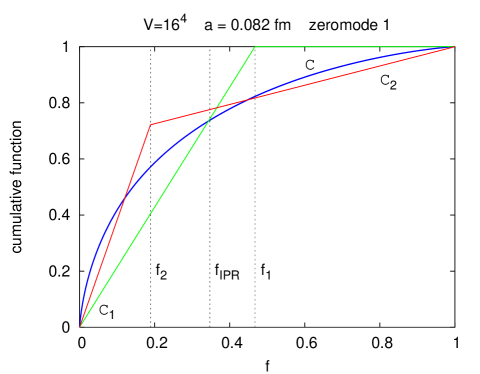
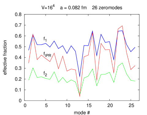
Figure 5: Left: The cumulative function ${\cal C}(f)$ for zero mode #1 and the associated effective fractions $f_{1}$ (with ${\cal C}_{1}(f)$), $f_{2}$ (with ${\cal C}_{2}(f)$), and $f_{IPR}$ are shown. Right: Three generic definitions of effective fraction discussed in the text for all 26 zero modes.

As can be seen clearly on the example of the overlap Dirac zero mode in Fig. 5 (left), the above generic definitions, while quite sensible for their designed purpose, give wildly different estimates for what the effective fraction is. It is thus potentially dangerous to use generic methods to determine the effective fraction in situations where sufficiently detailed characteristics of typical space-time distributions are not known, while the quantitative aspects of the problem are important. In particular, it would not be possible to seriously address the issues of global behavior in QCD vacuum at this stage by using a particular definition from the infinite set of generic possibilities available. At the same time, using a more complete information stored in the cumulative function makes it possible to resolve this issue.

Finally, we should emphasize that generic definitions, such as the above, are rather robust for comparative purposes, i.e. to decide if the support of mode $\psi_{1}$ is larger (more potent) than the support of mode $\psi_{2}$. Indeed, in Fig. 5 (right) we show the effective fractions for all $26$ modes using the above three definitions, and the comparisons are largely consistent.

References

- [1] I. Horváth, S.J. Dong, T. Draper, F.X. Lee, K.F. Liu, H.B. Thacker, J.B. Zhang, Phys. Rev. D67, 011501(R) (2003); I. Horváth et al., Nucl. Phys. B (Proc. Suppl.) 119, 688 (2003);
- [2] I. Horváth, S.J. Dong, T. Draper, F.X. Lee, K.F. Liu, N. Mathur, H.B. Thacker, J.B. Zhang, Phys. Rev. D68, 114505 (2003); I. Horváth et al., Nucl. Phys. B (Proc. Suppl.) 129&130, 677 (2004); I. Horváth et al., Proceedings of the “Quark Confinement and the Hadron Spectrum V”, Gargnano, Italy, Sep 10-14, 2002, N. Brambilla and G. Prosperi editors, World Scientific(2003) p.312, hep-lat/0212013.
- [3] I. Horváth, N. Isgur, J. McCune, H.B. Thacker, Phys. Rev. D65, 014502 (2002).
- [4] T. deGrand, A. Hasenfratz, Phys. Rev. D64, 034512 (2001).
- [5] I. Horváth, S.J. Dong, T. Draper, N. Isgur, F.X. Lee, K.F. Liu, J. McCune, H.B. Thacker, J.B. Zhang, Phys. Rev. D66, 034501 (2002).
- [6] T. DeGrand, A. Hasenfratz, Phys. Rev. D65, 014503 (2002); I. Hip et al., Phys. Rev. D65, 014506 (2002); R. Edwards, U. Heller, Phys. Rev. D65, 014505 (2002); T. Blum et al., Phys. Rev. D65, 014504 (2002); C. Gattringer et al., Nucl. Phys. B618 (2001) 205.
- [7] N. Cundy, M. Teper, U. Wenger, Phys. Rev. D66, 094505 (2002); C. Gattringer, Phys. Rev. Lett. 88 221601 (2002); P. Hasenfratz et al., Nucl. Phys. B643 (2002) 280; C. Gattringer, Phys. Rev. D67, 034507 (2003); C. Gattringer and R. Pullirsch, Phys. Rev. D69, 094510 (2004). T. Draper et al., hep-lat/0408006.
- [8] H. Neuberger, Phys. Lett B417 (1998) 141; Phys. Lett.B427 (1998) 353.
- [9] H. Thacker, S. Ahmad and J. Lenaghan, hep-lat/0409079.
- [10] P. Anderson, Phys. Rev. 109, 1492 (1958).
- [11] I. Horváth et al., in preparation.
- [12] E. Witten, Nucl. Phys. B156, 269 (1979); G. Veneziano, Nucl. Phys. B159, 213 (1979).
- [13] P. Hasenfratz, V. Laliena, F. Niedermayer, Phys. Lett. B427 (1998) 125.
- [14] R. Narayanan and H. Neuberger, Nucl. Phys. B443, 305 (1995).
- [15] I. Horváth, Talk at the workshop “The QCD Vacuum from a Lattice Perspective”, Jul 29–31 2004, Regensburg; I. Horváth et al., in preparation.
- [16] M. Guagnelli, R. Sommer, H. Wittig, Nucl. Phys. B535 (1998) 389.
- [17] Y. Chen et al., Phys. Rev. D70, 034502 (2004).
- [18] M. Golterman and Y. Shamir, Phys. Rev. D68, 074501 (2003).
- [19] F.V. Gubarev, A.V. Kovalenko, M.I. Polikarpov, S.N. Syritsyn and V.I. Zakharov, Phys. Lett. B574, 136 (2003); A.V. Kovalenko, M.I. Polikarpov, S.N. Syritsyn, V.I. Zakharov, hep-lat/0408014.
- [20] D.J. Thouless, Phys. Rep. 13 (1974) 93.
- [21] C. Gattringer et al. Nucl. Phys. B617, (2001) 101.
- [22] C. Aubin et al. [MILC], hep-lat/0410024.