Evidence for layered symmetry breaking in SU(2) lattice gauge theory

Abstract

Simulations of four-dimensional SU(2) lattice gauge theory are performed with partial axial gauge fixing trees spanning three of the four dimensions. The remaining SU(2) gauge symmetry, global in three directions and local in one, is found to break spontaneously at weak coupling, with the average fourth-dimension-pointing link in each perpendicular hyperplane as order parameter. The symmetry is restored at strong coupling. Symmetry breaking in each hyperplane appears to be independent, and occurs regardless of boundary conditions. The associated phase transition is likely coincident with the Polyakov loop transition.

1 Introduction

This paper presents evidence for a hidden symmetry breaking in 4-d SU(2) lattice gauge theory, made visible by a partial axial gauge fixing. The symmetry breaking occurs for weak coupling and the symmetry is restored at strong coupling, the two phases being separated by a phase transition. This transition is studied both on the Wilson axis and in the fundamental-adjoint plane[1] at an adjoint coupling of $\beta_{A}=1.5$. In the latter case, the transition is coincident with the previously-known first-order transition seen in the average plaquette, and also appears coincident with the Polyakov-loop deconfinement transition. The observed symmetry breaking provides an order parameter for this transition which remains valid with open boundary conditions, for which the Polyakov loop symmetry is absent. It also shows this bulk transition to be of the symmetry-breaking type. Symmetry-breaking bulk first-order transitions end in tricritical points rather than critical points, because a symmetry breaking transition must continue into the phase diagram in order to divide it completely into broken and unbroken regions which are not analytically connected. Indeed, evidence is found of a higher-order phase transition, with the same order parameter, on the Wilson axis in the crossover region. The existence of the bulk tricritical point to which this transition must attach, and the bulk nature of the order parameter (independent of boundary conditions) is strong evidence for this also being a bulk transition. On the Wilson axis, this is either coincident with or lies close to the Polyakov-loop transition on moderate size lattices up to $16^{4}$. Preliminary finite size scaling evidence favors the transition on the Wilson axis being of infinite-order, i.e. characterized by an essential singularity similar to the Berezinskii-Kosterlitz-Thouless (BKT) transition in the two-dimensional X-Y model[2]. It differs from this transition in having a symmetry-breaking order-parameter, made possible by the system having more than two dimensions. Below such a transition, the system is critical at every coupling, which is the expected behavior if the weak coupling phase is a massless-gluon phase characterized by an infinite-range force.

The existence of a bulk phase transition has important consequences for both the lattice and continuum theories. Simulations are relevant to the continuum theory only if they are run on the weak side of such a transition. Another alternative would be to identify the lattice artifacts which are responsible for the transition and devise a modified action that prohibits these artifacts or at least suppresses them enough to prevent the transition from occurring. Preliminary trials indicate that the system remains in the broken phase for all couplings with an action which prohibits both the SO(3)-Z2 monopoles defined in [3] as well as Z2 vortices (positive plaquette restriction). If the continuum limit is not confining, as confirmation of a bulk phase transition would imply, then it would make sense to suspect the quark sector of QCD as the true cause of confinement, perhaps as a side-effect of chiral symmetry breaking[4].

2 Motivation

The original motivation for this study was an apparent paradox in the 4-d Z2 lattice gauge theory. This theory is connected to SU(2) in the fundamental-adjoint plane [1] in the limit of infinite adjoint coupling. The Z2 theory undergoes a bulk first-order transition which is deconfining. The weak-coupling limit of this abelian theory is definitely not confined (no abelian theories are). The critical point is known from self-duality to be exactly $\beta_{c}=\frac{1}{2}\ln(1+\sqrt{2})\simeq 0.44$ [5]. The Polyakov loop serves as an order parameter for confinement, therefore it appears to be a proper order parameter for this transition. However, it, and the symmetry broken by it, are only defined with periodic boundary conditions. A bulk transition, on the other hand, should be independent of which boundary conditions are chosen. A symmetry-breaking first-order transition has a much different Landau free energy (even orders to sixth order present, with negative fourth-order term) than its non-symmetry-breaking cousin (third-order term driving transition). It is not reasonable to think changing the boundary conditions will have much effect on the free energy, a bulk quantity. Therefore, the transition must still be symmetry-breaking, even with open boundary conditions. But what is the order parameter and what symmetry is broken in this case? The current study began as a hunt for such an order parameter, as well as an order parameter for the attached first-order transition in the SU(2) fundamental-adjoint plane. Whether or not the latter is a symmetry-breaking transition is a subject of some controversy. Indirect evidence from the scaling of the latent heat with the size of the metastability region seems to indicate it is of the symmetry-breaking type[6]. Clear identification of a bulk symmetry-breaking order parameter associated with this transition would provide powerful confirmation of this idea. It is important because a symmetry-breaking first-order transition must end in a tricritical point (as opposed to an ordinary critical point). The transition then must continue from the tricritical point as a higher-order bulk transition which continues all the way through the phase plane, separating the plane into distinct symmetry-broken and symmetry-unbroken regions. The strong-coupling confining phase could not, in this case, be analytically connected to the weak coupling phase, but would be everywhere separated by a phase transition, contrary to the conventional picture.

It is well known that, although physical observables are gauge invariant, many important features in understanding the behavior of gauge theories are only observable in a fixed gauge. It is also well known, from Elitzur’s theorem, that a local gauge symmetry cannot be spontaneously broken [7]. The logic followed in this paper is to fix the gauge enough to invalidate Elitzur’s theorem, and see if any portion of the remaining exact partially-global gauge symmetry is broken spontaneously. If so, then one has found a broken symmetry and associated order parameter. This is somewhat reminiscent of symmetry breaking in the standard model except that there are no fields here besides the gauge fields. The gauge chosen is an axial gauge where all links on a tree (connected set of links with no loops) are set to one. The tree chosen is not the usual maximal tree, but rather the maximal tree with the last line of links pointing in the fourth direction left off, leaving $N$ disjoint trees. This leaves N independent exact SU(2) gauge symmetries (on an $N^{4}$ lattice), which operate “globally” on 3-d hyperplanes of fixed $x_{4}$ (coordinate in fourth direction). It is these symmetries which appear to be spontaneously broken at weak coupling and undergo a phase transition to an unbroken state at strong coupling. The order parameters are simply the layered-magnetizations formed from averaging the SU(2) links pointing in the fourth direction that lie in each hyperplane. Each hyperplane is in a sense acting like a 3-d O(4) Heisenberg model, linked to other intersecting and adjacent hyperplanes through the gauge couplings. Indeed, in two dimensions, the SU(2) gauge theory in the axial gauge actually splits into N non-interacting 1-d O(4) Heisenberg models[8]. Because the links in the opposite direction are all set to one, the four-link gauge couplings turn into two-link spin couplings. The same thing still happens for the 4-1 plaquettes of the 4-d theory, but not for the 4-2 or 4-3 plaquettes, also connected to the 4-links. Nevertheless, it might still make sense to think the 4-d theory as a set of 3-d Heisenberg models with additional interactions. These interactions may make the critical behavior different from that of the corresponding Heisenberg model.

3 Results and Analysis

Writing each SU(2) link as $a_{0}+ia_{1}\tau_{1}+ia_{2}\tau_{2}+ia_{3}\tau_{3}$ subject to the constraint $\sum_{k=0}^{3}a_{k}^{2}=1$, they can be pictured as unit 4-d vectors in the color parameter space. These vectors, for links pointing in the fourth spatial direction, are averaged over each $x_{4}=\rm{const.}$ hyperplane, to obtain $N$ magnetization color-vectors $\vec{m}_{i}$, $i=1\cdots N$, normalized per link. In the unbroken phase, these magnetizations sum to small random values consistent with Gaussian fluctuations around zero. In the broken phase they take on larger values, which drift slowly with Monte Carlo time, fluctuating around a nonzero magnitude and avoiding values near zero. In finite-lattice simulations one always has the problem that due to tunneling between broken vacua (the slow drift mentioned above) the order parameter itself will average to zero also in the broken phase. To distinguish the phases one can either monitor the magnitude of the magnetization or introduce a small explicit symmetry breaking through an external field. Both approaches are shown here.

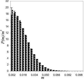
Figure 1: Histograms for (a) $\beta_{A}=1.5$, $\beta=1.0$, just on the strong coupling side and (b) $\beta_{A}=1.5$, $\beta=1.09$, just on the weak coupling side of the first order transition in the fundamental-adjoint plane. Error bars are from binned fluctuations. Striped bars in (a) are a fit to a Gaussian centered on zero. All histograms are arbitrarily normalized to integrate to unity. Labels on horizontal axis give middle of bin for every fourth bin, beginning with the first.

The phase transition is, of course, most visible when it is first order, so the first case to be considered is in the fundamental-adjoint plane with adjoint coupling $\beta_{A}=1.5$. This is below the triple-point but in a place where there is a fairly strong first-order transition with a jump of about $0.27$ in the average plaquette across the transition[6]. For the four-dimensional order parameter one must take into account the geometrical factor (from solid angle) that biases the distribution toward larger magnitudes. In the unbroken phase, the distribution of magnetization magnitudes, $m$, is expected to be a factor of $m^{3}$ times a Gaussian, $\exp(-m^{2}/2\sigma_{m}^{2})$. To more easily see the Gaussian behavior, the probability distribution $P(m)$ is obtained by histogramming, and the quantity $P(m)/m^{3}$ is plotted in Fig. 1, for the cases $\beta=1.00$, on the strong coupling side, and $\beta=1.09$, on the weak coupling side of the transition, which occurs around $\beta=1.04$. Here $\beta$ is the fundamental coupling parameter. In the first case the data fit well to the expected Gaussian peaked at zero. The value of $m$ for each bin is not taken at the center, but at a value that would produce a flat histogram in an $m^{3}$ distribution, regardless of bin-size choice. This is

$$m^{3}_{\rm{bin}}=\frac{1}{4}\frac{(m_{2}^{4}-m_{1}^{4})}{(m_{2}-m_{1})}.$$ (1)

where $m_{2}$ and $m_{1}$ are the bin edges. This detail affects only the first couple of bins in the histograms shown, and is necessary to get good Gaussian fits in the symmetric phase.

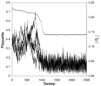
Figure 2: Time history of a tunneling event on a $12^{4}$ lattice. A lattice originally equilibrated at $\beta_{A}=1.5$, $\beta=1.09$, was subjected to a sudden change in fundamental coupling to $\beta=1.01$ at time labeled zero in graphs. Upper curve is average plaquette in both graphs. Lower curves in (a) are average link magnetizations for a sample of four of the twelve layers. Lower curve in (b) is the average Polyakov loop.

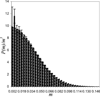
Figure 4: Histograms for Wilson-axis simulations at (a) $\beta=2.4$, (b) $\beta=2.9$, (c) $\beta=3.2$, (d) $\beta=3.2$ with open boundary conditions, and (e) $\beta=3.8$ on a $16^{4}$ lattice. Other runs are on a $12^{4}$ lattice and all but (d) are with periodic boundary conditions. Striped bins in (a) are a fit to a Gaussian centered on zero. Fit is to the first 12 bins. Extreme tail of data in (a) is somewhat lower than Gaussian would predict.

On the weak-coupling side of the transition, however, the distribution shows a definite non-zero peak, indicative of spontaneous symmetry breaking. This data was taken on a $12^{4}$ lattice with 5000 equilibration sweeps followed by 50,000 measurement sweeps. The 12 magnetizations on the different lattice layers behave identically, as they must due to translational symmetry with periodic boundary conditions. Their magnetization directions are random and they appear uncorrelated with each other, although detailed correlation analyses have not yet been performed. Each is treated as an independent measurement in the histogram. Fig. 2 shows a run which was first equilibrated at 1.09, with the beta value then abruptly changed to 1.01. One expects a period of metastability followed by an eventual tunneling to the symmetric phase. By watching the tunnelings of various quantities occur, one can get an idea of how closely they are correlated. In Fig. 2a, the plaquette and a sample of four of the twelve link magnetizations are shown. The others behave similarly. The unbreaking of the symmetries appears to occur just as the plaquette tunnels to its lower value in the unbroken phase. Fig. 2b shows the same for the Polyakov loop, which also appears to enter the restored-symmetry phase at the same time. The Polyakov loop may in some sense be measuring the product of the N magnetizations, but this relationship needs further exploration. Simulations at $\beta=1.09$ and $\beta=1.0$ were also performed with an open boundary condition (BC) in the fourth direction. The results for layers located more than two lattice spacings from the open boundary are close to those given above. For instance the average magnetization at $\beta=1.09$ with periodic BC’s was $0.149(2)$, and with open BC’s, 0.146(3). However the histograms are somewhat different. The histogram for open boundary conditions at this coupling (again ignoring layers near the boundary) picks up a second peak close to zero. Due to the $m^{-3}$ multiplying factor, only a few occurrences of near-zero magnetization can result in a peak here. Examination of the runs shows a few brief excursions near zero for some of the layers, which might be interpreted as “tunneling attempts”. Probably what has happened is that the open BC has shifted the critical point up a bit to the point where tunneling is beginning to occur. A simulation at a slightly weaker coupling, $\beta=1.3$, $\beta_{A}=1.5$, shows a very definite symmetry-broken histogram (Fig. 3), similar to Fig. 1b. Open boundary condition runs with the Wilson action (see Fig. 4c,d below) also give very similar histograms to periodic boundary condition runs at the same coupling. Thus boundary conditions are apparently not fundamentally important in this transition. The symmetry is still defined and still breaks at the transition, supporting the bulk nature of the transition. It should be noted that only the relevant boundary in the 4th direction, where the symetry breaking is being examined, was opened in these runs. The other directions had periodic boundary conditions.

Simulations were also run on the Wilson axis. Here a higher-order transition is expected. No bulk transition has previously been seen here at all – only the Polyakov loop transition which has been interpreted as a finite temperature transition, one which disappears on an infinite 4-d lattice. However, since a bulk symmetry is now seen to be breaking elsewhere in the fundamental-adjoint plane it must also be breaking here. Fig. 4 shows histograms for $12^{4}$ Wilson-axis runs at $\beta=2.4$, 2.9, 3.2, and a $16^{4}$ run at $\beta=3.8$. The former is seen to be unbroken and the latter all broken. Also shown (Fig. 5) are runs taken with an external field term of the form $-a_{0}h$ for each fourth-dimension-pointing link added to the action (this term is not multiplied by $\beta$). Here the $a_{0}$-component of magnetization is plotted as well as the magnitude. Only a small external field is needed to order the magnetization in the broken phase, which clearly extrapolates to a non-zero value in the limit of zero field. In contrast, in the unbroken phase ($\beta=2.2$) the magnetization extrapolates nearly linearly to zero. In determining what constitutes a “strong” or “weak” field, the magnitude of $h$ should be compared to $\beta$ since both links and plaquettes range from -1 to 1. The transition is consistent with being coincident with the deconfinement transition, which on a $12\times\infty^{3}$ lattice is projected to be at a $\beta_{c}$ of 2.64 [9]. However, the location of both transitions on the finite $12^{4}$ lattice is quite fuzzy, so a precise statement of coincidence is not possible at this time. It should be noted, however, that the layer spin magnetization breaks the Z2 Polyakov loop symmetry as well as the aforementioned gauge symmetry when it takes a non-zero expectation value. Without the $Z2$ symmetry to protect it, the Polyakov loop would be expected to also take an expectation value in this phase. Therefore it is extremely doubtful that the Polyakov loop transition could lie at a weaker coupling than the layered SU(2) transition. It could, however, lie at a stronger coupling, since restoration of the gauge symmetry does not necessarily imply restoration of the Z2 Polyakov loop symmetry.

Generally, the “finite lattice transition point” can be identified with a peak in the susceptibility, defined for the magnetization magnitude as

$$\chi=N^{3}(<m^{2}>-<m>^{2}).$$ (2)

However, for this system, Fig. 6 shows the susceptibility continues to rise at the weak coupling side of the transition (the $12^{4}$ lattice is broken beyond about $\beta=2.6$ and the $16^{4}$ beyond 2.8). Below $\beta=2.6$ all lattices give the same result, whereas at higher $\beta$ a large lattice-size dependence is seen, consistent with a possible divergence in the limit of infinite lattice size. Divergence without a peak is a possible indication of the system being critical at every $\beta$ above the transition (a massless phase), as would occur at a BKT-like transition. Indeed, $\chi$ for the 2-d XY model also does not peak at the critical point, but continues to rise in the low-temperature phase [10], and appears to be divergent everywhere there. Finite size scaling expected for such a transition is $\chi\propto N^{2-\eta}$, where $\eta$ is defined by the correlation function in the weak-coupling phase which is $\propto(x-x^{\prime})^{-\eta}$ [11]. Finite size scaling analysis between $8^{4}$, $12^{4}$ and $16^{4}$ lattices does not appear to be consistent with a power law. The $8^{4}$ lattice appears to have saturated and is probably simply too small to provide any information on asymptotic behavior. Such saturation is not a surprise, since $<m>$ is bounded by unity and its fluctuations are similarly bounded. Above $\beta=3.8$, the $12^{4}$ and $16^{4}$ lattices are marginally consistent with $\eta=1$, but the errors are large. One obtains $\eta=0.84\pm 0.18$, $1.25\pm 0.21$, and $1.24\pm 0.23$ at $\beta$ = 4.2, 4.5, and 5.0 respectively. If these are combined, the result is $1.08\pm 0.12$. Clearly higher statistics and larger lattices will be needed to measure the critical exponents with reasonable accuracy, and indeed to verify the nature of the criticality. If the system were scaling as the O(4) 3-d Heisenberg model, the prediction would be $\chi\propto N^{1.975}$ [12], which appears to be ruled out. A peak would also be expected in this case.

Finally, the Binder parameter[13],

$$U=1-<m^{4}>/(3<m^{2}>^{2})$$ (3)

is considered. For a finite-order transition, curves of the Binder parameter should cross at the infinite lattice transition point, at least in the limit of large lattices (next to leading corrections to scaling may make the smaller lattices miss the intersection somewhat). For the infinite order BKT-like transition, the Binder parameters for different size lattices do not cross, but merge, in the weak-coupling phase, because the system is critical throughout this phase (not just at the critical point). Fig. 7 shows the Binder parameter for this system on the three lattices. For an O(4) order parameter, the expected value for the Binder parameter in the random phase is $\frac{1}{2}$, and $\frac{2}{3}$ in a fully-ordered phase[14]. At criticality, the value should be a critical value somewhere in between these, which, except for higher order corrections, should be the same on all lattices. For a BKT transition, which is critical at every coupling in the weak-coupling phase, the critical $U$ could be a function of $\beta$. At strong coupling, $U$ for the larger lattices moves down strongly, consistent with approaching the expected value of $\frac{1}{2}$ in the symmetric phase. $U$ rises rapidly up to around $\beta=3.5$, after which it rises more slowly, with the larger lattices always below the smaller. There is no evidence for crossing or for large lattices approaching $\frac{2}{3}$, even far into the symmetry-broken region, as would be the case for an ordinary finite-order transition. The behavior is consistent with a massless phase beginning at a BKT-like transition which has an infinite-lattice transition point somewhere around $\beta=3.5$ to $4.0$. However, there is still way too much finite-lattice dependence to determine the critical values from these data – larger lattices will be needed.

Another quantity which seems to favor the existence of a BKT-like transition is the (pseudo) specific heat. The SU(2) theory has a large non-singular peak in the specific heat around $\beta=2.25$ which does not grow with lattice size[15]. Interestingly this is precisely the behavior of the X-Y model specific heat [10, 16], which has a large nonsingular peak displaced a long way from the critical point. The essential singularity at the critical point is very soft and not visible in numerical simulations. It is located where the specific heat begins its rise on the weak-coupling side of the peak. The X-Y model also has a very large finite-lattice shift in the critical point, due to the infinite-order scaling[10]. This could also explain the large $\beta$-shift seen in the deconfinement transition of the SU(2) gauge theory.

Some particulars of the simulations are as follows. Most runs were for 50,000 sweeps with 5000 equilibration sweeps for the $8^{4}$ and $12^{4}$ lattices, and 10,000 equilibration sweeps for the $16^{4}$ lattice. A Metropolis Monte Carlo algorithm was employed with acceptance kept between 0.3 and 0.7. Measurements were taken after every sweep. Equilibration times were set to twice the time it appeared to take for observables to equilibrate. The last observable to equilibrate was generally the Polyakov loop in the first direction, where all but one link are set to unity in this gauge. It takes some time for the information to percolate into that one link, definitely more than for the Polyakov loop to equilibrate in the non-gauge-fixed case, but not an unreasonably long time. For $\beta=4.2$ and above, 100,000 measurement sweeps were taken. Runs with an external field present (Fig. 5) were shorter, only 5000 measurement sweeps, because the magnetization itself (as opposed to its moments) is fairly easily measured.

4 Conclusion

In conclusion, a symmetry breaking phase transition is seen on 3-d layers of 4-d SU(2) lattice gauge theory in a partially-fixed axial gauge. The symmetry broken is the remaining exact SU(2) global gauge symmetry on each layer, with the order parameter being the link magnetization in the unfixed direction on each perpendicular hyperplane. The transition also remains for the case of open boundary conditions. The lack of dependence on boundary conditions, the bulk nature of the order parameter (existing locally on all layers rather than globally in the fourth direction or on a single surface) and the apparent coincidence of the transition with the bulk first-order transition in the fundamental-adjoint coupling plane, strongly support this being a bulk transition. Finite-size scaling of the susceptibility and Binder parameter suggest a BKT-like transition with the system being in a massless phase for all couplings smaller than the critical coupling, including the continuum limit.

It is interesting to consider if this symmetry breaking has implications for the continuum theory, since the continuum limit is in the symmetry-broken phase. Normally no part of the gauge symmetry is thought to be spontaneously broken in the continuum pure-gauge theory. However, this work would seem to indicate that the gauge fields themselves can and do break a portion of the (partially global) gauge symmetry remaining after partial gauge fixing. The gauge fields observed in nature could be the Goldstone bosons associated with this symmetry breaking. It is not clear whether this has any physical implications or whether it is simply a different way of looking at the continuum gauge theory resulting from the choice of gauge.

It is also very interesting to consider what would happen if the gauge fixing were further relaxed, by fixing aong only the first two directions. Such an investigation is being planned. This would leave $N^{2}$ exact SU(2) symmetries which are global on two-dimensional planes of fixed ($x_{3}$,$x_{4}$). There would be two order parameters, the link magnetizations in both the 3 and 4 directions. However, it is unclear whether these could break spontaneously or not, due to the two-dimensionality of the layers. In a true two-dimensional system, the Mermin-Wagner theorem prevents spontaneous breaking of a continuous symmetry. Here, however, the two-dimensional layers are linked to others. It is possible that a phase transition on these underlying two-dimensional layers is how BKT-like behavior finds its way into a four-dimensional theory.

Figure 3: Histogram for $\beta_{A}=1.5$, $\beta=1.3$ with open boundary conditions. The two closest layers on both sides of the boundary (a total of four layers) are excluded. The first bin is empty.

Figure 5: Effect of imposing an external field, $h$, coupled to 0-component of magnetization, here called $m_{0}$ and plotted as triangles. Also shown is the magnetization magnitude, $m$, plotted as squares. Solid symbols are for $12^{4}$ lattice and open are for $16^{4}$. Lower data set is for $\beta=2.2$, and upper two are for $\beta=2.9$ on the two different lattices. Lines are linear fits to $<m_{0}>$ in the range $0.0375\leq h\leq 0.075$ where this quantity is nearly linear. The $\beta=2.9$ data clearly extrapolate to non-zero values at zero external field, which, for the $16^{4}$ lattice, is close to the zero-field value of $<m>$. This is the expected hysteresis curve for a broken symmetry. The 0-component of magnetization for $\beta=2.2$ extrapolates to a point consistent with zero, as expected in the symmetric phase.

Figure 6: Susceptibility vs. $\beta$ for $8^{4}$ (diamonds), $12^{4}$ (squares) and $16^{4}$ (triangles) lattices.

Figure 7: Binder parameter for $8^{4}$ (diamonds), $12^{4}$ (squares), and $16^{4}$ (triangles) lattices. Prediction for large lattices in the symmetric phase is 0.5 and in a broken phase for a finite-order transition is 0.667. Critical values are expected to lie between these two extremes.

References

- [1] G. Bhanot and M. Creutz, Phys. Rev. D 24, 3212 (1981).
- [2] V.L. Berezinskii, Sov. Phys. JETP 32, 493 (1970); J.M. Kosterlitz and D.J. Thouless, J. Phys. C 6, 1181 (1973); J.M. Kosterlitz, J. Phys. C 7, 1046 (1974).
- [3] M. Grady, report SUNY-FRE-98-09, hep-lat/9806024 (1998).
- [4] V.N. Gribov, Phys. Scr. T15, 164 (1987), Phys. Lett. B 194, 119 (1987); J. Nyiri, ed., The Gribov Theory of Quark Confinement, World Scientific, Singapore, 2001; M. Grady, Z. Phys C, 39, 125 (1988), Nuovo Cim. 105A, 1065 (1992); K. Cahill and G. Herling, Nucl. Phys. B Proc. Suppl. 73, 886 (1999); K. Cahill, report NMCPP/99-7, hep-ph/9901285.
- [5] F.J. Wegner, J. Math. Phys. 12, 2259 (1971).
- [6] M. Grady, report SUNY-FRE-04-02, hep-lat/0404015 (2004).
- [7] S. Elitzur, Phys. Rev. D 12, 3978 (1975).
- [8] This construction is demonstrated for the Z2 theory in J.B. Kogut, Rev. Mod. Phys. 51, 659 (1979).
- [9] I.L. Bogolubsky et. al.,Nucl. Phys. B (Proc. Suppl.) 129&130, 611 (2004).
- [10] J. Tobochnik and G.V. Chester, Phys. Rev. B 20, 3761 (1979); R. Gupta et. al., Phys. Rev. Lett. 61, 1996 (1988); R. Gupta and C.F. Baillie, Phys, Rev. B 45, 2883 (1992).
- [11] M.N. Barber in Phase Transitions and Critical Phenomena, Vol. 8, C. Domb and J.L. Liebowitz, ed., Academic Press, New York, 1983, pp 192-195.
- [12] K. Kanaya and S. Kaya, Phys. Rev. D 51, 2404 (1995).
- [13] K. Binder, Z. Phys. B - Condensed Matter 43, 119 (1981).
- [14] C. Holm and W. Janke, Phys. Rev. B 48, 936 (1993).
- [15] Modern high-statistics data for the SU(2) specific heat is available in J. Engels and T. Scheideler, Nucl. Phys. B (Proc. Suppl.) 53, 423 (1997).
- [16] P.M. Chaiken and T.C. Lubensky, Principles of Condensed Matter Physics, Cambridge University Press, Cambridge, 1995, p. 550.