DESY 04-189 LU-ITP 2004/029 Edinburgh 2004/21 Generalized parton distributions and structure functions from full lattice QCD

Abstract

We present here the latest results from the QCDSF collaboration for (moments of) structure functions and generalized form factors in full QCD with $N_{\rm f}=2$ ${\cal O}(a)$-improved Wilson fermions based on simulations closer to the chiral and continuum limit.

1 INTRODUCTION

Understanding the internal structure of hadrons in terms of quarks and gluons (partons), and in particular how these provide the binding and spin of the nucleon, is one of the outstanding problems in particle physics.

Matrix elements of the light cone operator

$${\cal O}(x)=\int\frac{d\lambda}{4\pi}\; e^{i\lambda x}\;\overline{q}(-\frac{\lambda}{2}n)\not\!n$$ (1)

$${\cal P}e^{\!-ig\int^{\lambda/2}_{-\lambda/2}d\alpha\,n\cdot A(\alpha n)}q(\frac{\lambda}{2}n)$$

measured in deep-inelastic scattering experiments provide a wealth of information regarding the quark and gluon content of the nucleon.

Expanding ${\cal O}(x)$ in terms of local operators via the operator product expansion generates the tower of twist-2 operators

$${\cal O}^{\{\mu_{1}\cdots\mu_{n}\}}=\overline{q}\,i\,\gamma^{\{\mu_{1}}\,\stackrel{{\scriptstyle\leftrightarrow}}{{D}}^{\mu_{2}}\cdots\stackrel{{\scriptstyle\leftrightarrow}}{{D}}^{\mu_{n}\}}\!q\ ,$$ (2)

where $\stackrel{{\scriptstyle\leftrightarrow}}{{D}}=\frac{1}{2}(\overrightarrow{D}-\overleftarrow{D})$ and $\{\cdots\}$ indicates symmetrization of indices and removal of traces. The (non-)forward matrix elements of Eq. (2) specify the $(n-1)^{th}$ moments of the (generalized) parton distributions.

Parton distributions measure the probability $|\psi(x)|^{2}$ of finding a parton with fractional longitudinal momentum $x$ in the fast moving nucleon at a given transverse resolution $1/Q$. Generalized parton distributions (GPDs) [1, 2] describe the coherence of two different hadron wave functions $\psi^{\dagger}(x+\xi/2)\,\psi(x-\xi/2)$, one where the parton carries fractional momentum $x+\xi/2$ and one where this fraction is $x-\xi/2$, from which further information on the transverse distribution of partons can be drawn [3, 4]. In the limit where the momentum transfer $\Delta$ to the nucleon is purely transverse, i.e. $\Delta=(0,\vec{\Delta}_{\perp})$ and $\xi=0$, GPDs regain a probabilistic interpretation [4]. In the forward limit ($\Delta=0$), these distributions reduce to the Feynman parton distributions.

Moments of GPDs are amenable to lattice calculations [5, 6, 7]. Thus, they offer a promising way to link phenomenological observations to first principle theoretical considerations. In this talk we report on recent unquenched results obtained by the QCDSF collaboration.

2 SIMULATION DETAILS

We simulate with $N_{\rm f}=2$ dynamical configurations generated with Wilson glue and non-perturbatively ${\cal O}(a)$ improved Wilson fermions. For five different values $\beta=5.20$, $5.25$, $5.26$, $5.29$, $5.40$ and up to three different kappa values per beta we have in collaboration with UKQCD generated ${\cal O}(2000-8000)$ trajectories. Lattice spacings and spatial volumes vary between 0.075-0.123 fm and (1.5-2.2 fm)³ respectively.

Correlation functions are calculated on configurations taken at a distance of 5-10 trajectories using 8-4 different locations of the fermion source. We use binning to obtain an effective distance of 20 trajectories. The size of the bins has little effect on the error, which indicates auto-correlations are small. This work improves on previous calculations by adding one more sink momentum, $\vec{p}_{2}$, and polarization, $\Gamma_{1}$. We use $\vec{p}_{0}=(0,0,0)$, $\vec{p}_{1}=(p,0,0)$, $\vec{p}_{2}=(0,p,0)$ ($p=2\pi/L_{S}$) and $\Gamma_{\rm unpol}=\frac{1}{2}(1+\gamma_{4})$, $\Gamma_{1}=\frac{1}{2}(1+\gamma_{4})\,i\gamma_{5}\gamma_{1}$, $\Gamma_{2}=\frac{1}{2}(1+\gamma_{4})\,i\gamma_{5}\gamma_{2}$.

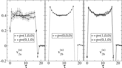
Figure 1: Bare results for the lowest moment of $F_{2}$ at $(\beta,\kappa_{\rm sea})=(5.4,0.13560)$, $t=17$. The fat horizontal lines are obtained from a fit to the data. $v_{\rm 2a}$ and $v_{\rm 2b}$ refer to different lattice versions of the same operator.

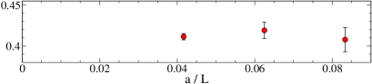
Figure 2: Finite size analysis for $v_{2b}^{\rm RGI}$ ($\vec{p}=(0,0,0)$) at $(\beta,\kappa_{\rm sea})=(5.29,0.13550)$ on $V=24^{3}\times 48$, $16^{3}\times 32$, $12^{3}\times 32$ lattices.

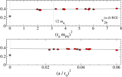
Figure 3: Results from a fit to Eq. (6) with $\Lambda_{\chi}=0$. The upper plot shows the chiral extrapolation $v_{2b}^{\rm RGI}(r_{0},m_{\rm PS})-c_{2b}(a/r_{0})^{2}$ and the lower plot the continuum extrapolation $v_{2b}^{\rm RGI}(r_{0},m_{\rm PS})-F^{v_{2b}}(r_{0}m_{\rm PS})$.

3 QUARK DISTRIBUTIONS

The moments of the $F_{2}$ structure function $\langle x^{n-1}\rangle$ are determined by calculating the matrix elements

$$\langle N(\vec{p})|\left[{\cal O}^{\{\mu_{1}\cdots\mu_{n}\}}_{q}-{\rm Tr}\right]|N(\vec{p})\rangle^{\cal S}=\\ 2v_{n}^{(q){\cal S}}(g^{\cal S}({\cal M}))\;[p^{\mu_{1}}\cdots p^{\mu_{n}}-{\rm Tr}],$$ (3)

and corresponding Wilson coefficients in a renormalization scheme $\cal S$ (eg. $\overline{\rm MS}$) and at a scale $\cal M$ (e.g. 2 GeV). See [8] for the operators to use on the lattice. To eliminate ${\cal O}(a)$ terms in the matrix elements, these operators need to be improved. For the lowest moment, i.e. $v_{2}$, this amounts to replacing ${\cal O}^{\gamma}_{\mu\nu}$ by $(1+am_{\rm q}c_{0})\;{\cal O}^{\gamma}_{\mu\nu}+\sum_{i=1}^{2}a\,c_{i}\;{\cal O}^{(i)}_{\mu\nu}$. The improvement coefficient $c_{0}$ is only known perturbatively, while the other coefficients are unknown. Since the corresponding operator matrix elements turn out to be negligible we will set $c_{1}=c_{2}=0$. For the higher moments an additional problem arises: the operators may mix with operators with total derivatives [9]. However, the corresponding operators are again found to be small and are therefore neglected here.

Matrix elements are determined from the ratio of three-point to two-point correlation functions

$${\cal R}(t,\tau;\vec{p}\,^{\prime},\vec{p};{\cal O})\,=\frac{C_{\Gamma}(t,\tau;\vec{p}\,^{\prime},\vec{p},{\cal O})}{C_{2}(t,\vec{p}\,^{\prime})}$$

$$\times\left[\frac{C_{2}(\tau,\vec{p}\,^{\prime})C_{2}(t,\vec{p}\,^{\prime})C_{2}(t-\tau,\vec{p}\,)}{C_{2}(\tau,\vec{p}\,)C_{2}(t,\vec{p}\,)C_{2}(t-\tau,\vec{p}\,^{\prime})}\right]^{\frac{1}{2}}$$

where $C_{2}$ is the unpolarized baryon two-point function with a source at time 0 and sink at time $t$, while the unpolarized three-point function $C_{\Gamma}$ has an operator ${\cal O}$ insertion at time $\tau$. For the matrix elements $v_{n}$ we have $\vec{p}=\vec{p}\,^{\prime}$, i.e. the last term of Eq. (3) is equal to 1. To improve our signal for non-zero momentum we average over the results for $C_{\Gamma}$ and $C_{2}$ for both momenta before we calculate the ratio $\cal R$. In Fig. 1 we compare the results for the different ways of obtaining the lowest moment. Within errors the results are consistent.

The bare matrix elements must be renormalized. While non-perturbatively determined renormalization factors are known in quenched QCD [10], the situation for dynamical simulations is still under investigation. Here we use tadpole-improved renormalization-group-improved boosted perturbation theory [11] to convert our lattice results to RGI.

Before we examine the quark mass and lattice spacing behaviour of our results, we first check for finite size effects. In Fig. 2 we present the first results of a finite size analysis for $v_{2b}$. Here we plot $v_{2b}$ as a function of inverse spatial lattice extent for three different volumes $V=24^{3}\times 48$, $16^{3}\times 32$, $12^{3}\times 32$ at $(\beta,\kappa_{\rm sea})=(5.29,0.13550)$. This preliminary analysis reveals that the finite size effects for $v_{2b}$ are small.

Finally, the discretization effects and quark mass dependence need to be investigated. The commonly accepted procedure is to first extrapolate to the continuum limit then to the chiral limit. Since the currently available data does not allow us to perform both extrapolations separately, we make the following ansatz for a simultaneous chiral and continuum extrapolation:

$$v_{n}^{\rm RGI}(r_{0},m_{\rm PS})=F^{v_{n}}(r_{0}m_{\rm PS})\;+\\ c_{n}\,\left(\frac{a}{r_{0}}\right)^{2}+d_{n}\,ar_{0}\,m_{\rm PS}^{2}.$$ (5)

The terms proportional to $c_{n}$ and $d_{n}$ take discretization errors $\propto a^{2}$ and residual effects $\propto am_{q}$ into account (we fix $d_{n}=0$). The first term corresponds to a chiral extrapolation. To incorporate chiral physics into the extrapolation taking into account the effects due to the ‘pion cloud’ surrounding the nucleon, the ansatz

$$F^{v_{n}}(x)=v_{n}^{\rm RGI}\left(1-cx^{2}\ln\frac{x^{2}}{x^{2}+r_{0}^{2}\Lambda_{\chi}^{2}}\right)+a_{n}x^{2}$$ (6)

has been proposed [12], where $c\approx 0.663$ and $\Lambda_{\chi}$ is a free parameter, usually taken to be of ${\cal O}(1\,{\rm GeV})$. Setting $\Lambda_{\chi}=0$ reduces Eq. (6) to a linear extrapolation in $(r_{0}m_{\rm PS})^{2}$.

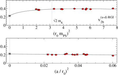
Figure 4: Same as Fig. 3 but for $\Lambda_{\chi}=1$ GeV.

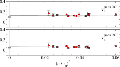
Figure 5: Continuum extrapolation of $v_{3}$ and $v_{4}$.

In Fig. 3, we plot the results for $v_{2b}^{\rm RGI}(r_{0},m_{\rm PS})-c_{2b}(a/r_{0})^{2}$ as calculated from Eq. (5) with $\Lambda_{\chi}=0$ ($\chi^{2}/{\rm d.o.f}=2$) and plotted as a function of $m_{\rm PS}^{2}$ for the isovector $u-d$. We see here that although our data at heavy quark masses agree very well with a linear extrapolation, the predicted value in the chiral limit is roughly twice the experimental value. A fit using Eq. (5) with $\Lambda_{\chi}=1$ GeV and the result in the chiral limit constrained to the experimental value does not describe our data equally well ($\chi^{2}/{\rm d.o.f}=5$). However, as can be seen from Fig. 4 any disagreement is not significant since all of the curvature of the fit occurs in the light quark mass region where there is no data. Even at our lightest quark mass ($m_{\rm PS}\approx 500$MeV) we are not yet into the region where curvature is expected to occur.

Turning our attention now to discretization effects, in the bottom figure of Fig. 4 we plot $v_{2b}^{\rm RGI}(r_{0},m_{\rm PS})-F^{v_{2b}}(r_{0}m_{\rm PS})$ as a function of $(a/r_{0})^{2}$. Here we observe a very small dependence on the lattice spacing, indicating that not only is our ${\cal O}(a)$ improvement program working, but also that ${\cal O}(a^{2})$ effects are small.

For the higher moments we only perform a chiral extrapolation linear in $(r_{0}m_{\rm PS})^{2}$. The results for $v_{3}$ and $v_{4}$ from the combined chiral and continuum extrapolation are shown in Fig. 5.

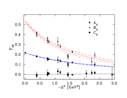
Figure 6: Generalized form factors $A^{u-d}_{20},\ B^{u-d}_{20}$ and $C^{u-d}_{2}$, together with a dipole fit.

4 GENERALIZED PARTON DISTRIBUTIONS

Non-forward matrix elements of the twist-2 operators in Eq. (2) yield the moments of generalized parton distributions

$$\!\!\int_{-1}^{1}dx\,x^{n-1}\,H_{q}(x,\xi,\Delta^{2})\!\! = \!\!H_{qn}(\xi,\Delta^{2})$$

$$\!\!\int_{-1}^{1}dx\,x^{n-1}\,E_{q}(x,\xi,\Delta^{2})\!\! = \!\!E_{qn}(\xi,\Delta^{2})$$ (7)

where [2]

$$H_{qn}(\xi,\Delta^{2}) = \sum_{i=0}^{\frac{n-1}{2}}A_{qn,2i}(\Delta^{2})(-2\xi)^{2i}$$

$$+ {\rm Mod}(n+1,2)C_{qn}(\Delta^{2})(-2\xi)^{n}$$

$$E_{qn}(\xi,\Delta^{2}) = \sum_{i=0}^{\frac{n-1}{2}}B_{qn,2i}(\Delta^{2})(-2\xi)^{2i}$$

$$- {\rm Mod}(n+1,2)C_{qn}(\Delta^{2})(-2\xi)^{n}$$

and the generalized form factors $A^{q}_{n,2i}(\Delta^{2})$, $B^{q}_{n,2i}(\Delta^{2})$ and $C^{q}_{n}(\Delta^{2})$ for the lowest three moments are extracted from the nucleon matrix elements $\langle p^{\prime}|{\cal O}^{\{\mu_{1}\cdots\mu_{n}\}}|p\rangle$ [2]. For the lowest moment, $A_{10}$ and $B_{10}$ are just the Dirac and Pauli form factors $F_{1}$ and $F_{2}$, respectively. We also observe that in the forward limit ($\Delta^{2}=\xi=0$), the moments of $H_{q}$ reduce to the moments of the unpolarized parton distribution $A_{n0}=\langle x^{n-1}\rangle$.

In order to extract the non-forward matrix elements we compute ratios of three- and two-point function as in Eq. (3) with $\vec{p}\neq\vec{p}\,^{\prime}$.

In Fig. 6 we show, as an example, the generalized form factors $A_{20},\ B_{20}$ and $C_{2}$ for the non-singlet, $u-d$, on a $24^{3}\times 48$ lattice at $\beta=5.40$ and $\kappa_{\rm sea}=\kappa_{\rm val}=0.13500$ corresponding to a lattice spacing, $a\,r_{0}=6.088$ and $m_{\rm PS}\approx 970$ MeV.

The generalized form factors $A_{20},\ B_{20}$ are well described by the dipole ansatz

$$A_{n}^{q}(\Delta^{2})=\frac{A_{n}^{q}(0)}{\big{(}1-{\Delta^{2}/M_{n}^{2}}\big{)}^{2}}\ ,$$ (9)

while $C^{u-d}_{2}$ is consistent with zero.

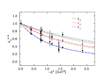
Figure 7: Generalized form factors $A^{u-d}_{10},\ A^{u-d}_{20}$ and $A^{u-d}_{30}$, together with a dipole fit. All form factors have been normalized to unity.

Burkardt [4] has shown that the spin-independent and spin-dependent generalized parton distributions $H(x,0,\Delta^{2})$ and $\widetilde{H}(x,0,\Delta^{2})$ gain a physical interpretation when Fourier transformed to impact parameter space

$$q(x,\vec{b}_{\perp})=\int\frac{d^{2}\Delta_{\perp}}{(2\pi)^{2}}\,{\rm e}^{-i\vec{b}_{\perp}\cdot\vec{\Delta}_{\perp}}H(x,0,-\Delta_{\perp}^{2})\,,$$ (10)

(and similar for the polarized $\Delta q(x,\vec{b}_{\perp})$) where $q(x,\vec{b}_{\perp})$ is the probability of finding a quark with longitudinal momentum fraction $x$ and at transverse position (or impact parameter) $\vec{b}_{\perp}$.

Burkardt [4] also argued that $H(x,0,-\Delta_{\perp}^{2})$ becomes $\Delta_{\perp}^{2}$-independent as $x\rightarrow 1$ since, physically, we expect the transverse size of the nucleon to decrease as $x$ increases, i.e. $\lim_{x\rightarrow 1}q(x,\vec{b}_{\perp})\propto\delta^{2}(\vec{b}_{\perp})$. As a result, we expect the slopes of the moments of $H(x,0,-\Delta_{\perp}^{2})$ in $\Delta_{\perp}^{2}$ to decrease as we proceed to higher moments. This is also true for the polarized moments of $\widetilde{H}(x,0,-\Delta_{\perp}^{2})$, so from Eq. (4) with $\xi=0$, we expect that the slopes of the generalized form factors $A_{n0}(\Delta^{2})$ and $\widetilde{A}_{n0}(\Delta^{2})$ should decrease with increasing $n$.

In Figs. 7 and 8, we show the $\Delta^{2}$-dependence of $A_{n0}(\Delta^{2})$ and $\widetilde{A}_{n0}(\Delta^{2})$, respectively for $n=1,2,3$. The form factors have been normalized to unity to make a comparison of the slopes easier and as in Fig 6 we fit the form factors with a dipole form as in Eq. (9). We note here that the form factors for the unpolarized moments are well separated and that their slopes do indeed decrease with increasing $n$ as predicted. For the polarized moments, we observe a similar scenario, however here the change in slope between the form factors is not as large. This is to be compared with the results from Ref. [7] which reveal no change in slope between the $n=2$ and $n=3$ polarized moments.

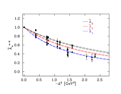
Figure 8: Same as Fig. 7 but for $\tilde{A}^{u-d}_{n0}$.

Although fitting the form factors with a dipole is purely phenomenological, it does provide us with a useful means to measure the change in slope of the form factors by monitoring the extracted dipole masses $(M_{1},\,M_{2},\,M_{3})$ as we proceed to higher moments. We have calculated these generalized form factors on a subset of our full complement of $(\beta,\,\kappa)$ combinations and have extracted the corresponding dipole masses. We plot these dipole masses in Fig. 9 as a function of $m_{\rm PS}^{2}$. Included for comparison are previous quenched results for the first [13] and second [5] moments. The new unquenched results indicate that quenching effects are small for form factors.

Figure 9: Dipole masses for the first three moments of $H(x,0,-\Delta_{\perp}^{2})$ as a function of $m_{\rm PS}^{2}$, together with a linear extrapolation to the physical pion mass.

The important feature to note in Fig. 9 is the distinct separation between (and increase in magnitude of) the dipole masses as we move to higher moments $(x\rightarrow 1)$. Although the data available for $M_{3}$ is limited, the behaviour of all dipole masses appears to be linear with $m_{\rm PS}^{2}$. Consequently, we perform individual linear extrapolations of the dipole masses $M_{1},\,M_{2},\,M_{3}$ to the physical pion mass, although the findings of Ref. [14] suggest that the chiral extrapolation of the dipole masses of the electromagnetic form factors may be non-linear.

If the dipole behavior Eq. (9) continues to hold for the higher moments as well, and if we assume that the dipole masses continue to grow in a Regge-like fashion, we may write

$$\int_{-1}^{1}\mbox{d}x\,x^{n-1}\,H_{q}(x,0,\Delta^{2})=\frac{\langle x_{q}^{n-1}\rangle}{(1-\Delta^{2}/M_{n}^{2})^{2}},$$ (11)

with $M_{l}^{2}=\mbox{const.}+l/\alpha^{\prime}$, where $\mbox{const.}\approx-0.5$ GeV² and $1/\alpha^{\prime}\approx 1.1$ GeV². This is sufficient to compute $H_{q}(x,0,\Delta^{2})$ by means of an inverse Mellin transform [15].

Having done so, the desired probability distribution of finding a parton of momentum fraction $x$ at the impact parameter $\vec{b}_{\perp}$ can then be obtained by the Fourier transform of Eq. (10).

5 CONCLUSION

We presented an update on our results for $\langle x^{n-1}\rangle$ in full QCD. While data closer to the chiral and continuum limit became available, the linear behaviour observed previously [16] still holds. Finally, we have shown preliminary results for the first 3 moments of the GPDs. Our data confirms the expected flattening going to higher moments.

References

- [1] D. Müller et al., Fortsch. Phys. 42, 101 (1994); A.V. Radyushkin, Phys. Rev. D56, 5524 (1997); M. Diehl et al., Phys. Lett. B411, 193 (1997).
- [2] X. Ji, Phys. Rev. Lett. 78, 610 (1997); X. Ji, J. Phys. G24, 1181 (1998).
- [3] M. Diehl, Eur. Phys. J. C25, 223 (2002).
- [4] M. Burkardt, Int. J. Mod. Phys. A18, 173 (2003).
- [5] M. Göckeler et al., hep-ph/0304249.
- [6] P. Hägler et al., Phys. Rev. D68 (2003) 034505.
- [7] P. Hägler et al., hep-lat/0312014.
- [8] M. Göckeler et al., in preparation.
- [9] M. Göckeler et al., hep-lat/0409025.
- [10] G. Martinelli et al., Nucl. Phys. B445 (1995) 81; M. Göckeler et al., Nucl. Phys. B544 (1999) 699; A. Shindler et al., hep-lat/0309181.
- [11] S. Capitani et al., Nucl. Phys. (Proc. Suppl.) 106 (2002) 299.
- [12] A.W. Thomas et al., Phys. Rev. Lett. 85, 2892 (2000); W. Detmold et al., Phys. Rev. Lett. 87, 172001 (2001).
- [13] M. Göckeler et al., hep-lat/0303019.
- [14] J.D. Ashley et al., hep-lat/0308024.
- [15] M. Göckeler et al., hep-ph/9711245.
- [16] T. Bakeyev et al., hep-lat/0311017.
- [17] C. R. Allton et al., Phys. Rev. D65 (2002) 054502, hep-lat/0107021.