Non leptonic two–body decay amplitudes from finite volume calculations

Abstract

We discuss the quantization of the energy levels of two–particle scattering states in a finite volume in the case of Bloch–type boundary conditions. A generalization of the Lüscher quantization condition is obtained that can be used in order to calculate the scattering phases, resulting for example by the strong elastic interaction of two pions, at fixed physical momentum transfers on a sequence of volumes of growing sizes. We also give a generalization of the Lellouch–Lüscher formula to be used to extract the physical $K\mapsto\pi\pi$ decay rate below the inelastic threshold from finite volume calculations. The formula is valid up to corrections exponentially vanishing in the volume. By using this formula the calculation can in principle be performed on different finite volumes of growing sizes in order to keep under control the corrections.

1 Introduction

The calculation of the weak matrix elements associated to the non–leptonic decay $K\mapsto\pi\pi$ requires a non–perturbative level of accuracy, due to the strong nature of the final state re–interactions. Lattice gauge theory is the best candidate among the other methods to achieve a phenomenologically relevant result for this process but there are theoretical problems that have to be addressed before such kind of calculations can be actually performed. The obstacles that have to be removed are mainly due to two different reasons.

The so called “ultraviolet problem”, concerning the construction of finite matrix elements of properly renormalized lattice operators, has been addressed by many authors and we will not discuss it further in the rest of this paper (see [1] for a recent review of this subject). Here we will focus our attention on the so called “infrared problem”.

The infrared problem, formalized in the well known Maiani–Testa “no–go” theorem [2, 3], concerns the impossibility of connecting the large time correlation functions calculated on a large euclidean volume with the physical decay amplitudes. A solution to the infrared problem has been found in ref. [4] where Lellouch and Lüscher (in the following referred as LL) derived a relation connecting the finite volume euclidean $K\mapsto\pi\pi$ matrix elements with the physical ones, up to exponentially small finite volume corrections.

The key point in the derivation of the LL formula is that the Maiani–Testa theorem applies in the case of very large volumes, where the spectrum of the two–particle final state is continuous, but ceases to be valid in the case of finite volumes where the two–particle energy is quantized. In the last case a kaon at rest cannot decay into two pions unless the physical extension of the finite volume is such that one of the two–particle energy levels equals the mass of the decaying particle. A simple phenomenological analysis based on the results of refs. [5, 6, 7, 8] shows that, when the two pions satisfy periodic boundary conditions, the volume on which the energy of the first excited state of definite isospin coincides with the kaon mass is of the order of $5.5$ fm. Such a large value of the volume makes the calculation unfeasible from the practical point of view due to the limiting present computer power. Furthermore the calculation is performed on a single finite volume and the corrections, although exponentially vanishing, cannot be quantified.

The authors of ref. [9] have shown that a set of LL formulas can be derived also when the energy of the outgoing two–pion state does not coincide with the kaon mass. In this case the resulting infinite volume decay rates are not calculated at the physical point, i.e. at the values of the two–pion energies fixed by relativistic kinematics. Nevertheless one can repeat the calculation for different finite volumes and then extrapolate the results to the physical point. In ref. [9] it has been also pointed out that the finite volume corrections to the LL formulas could result to be sizable if only few two–particle states have energies below the inelastic threshold.

In this paper we study the quantization condition of the energy of a two–particle state on a finite volume by using a generalized set of boundary conditions ($\theta$–BC) for the two particles. In ref. [10] we have shown that the use of $\theta$–BC in framework of lattice calculations makes possible a continuous momentum transfer between one–particle states. In the following we obtain a quantization condition for the energy of a two–particle state on a finite volume that generalize a result previously obtained by Lüscher [7] in the case of periodic boundary conditions. We also give a generalization of the LL formula and show that by using the $\theta$–dependence of this formula and of our quantization condition it is possible to find a sequence of finite volumes of growing sizes on which the calculation of the $K\mapsto\pi\pi$ decay rates can be performed at the physical point. Using the values of the scattering phases predicted by chiral perturbation theory we show that the physical amplitudes can be calculated on volumes of the order of about $3$ fm and, at the same time, the residual functional dependence of the results upon the volume can be quantified.

The plan of the paper is as follows. In section 2 we set up the notations. In section 3 we derive the quantization condition while the generalized LL formula is given in section 4. In section 5 we study the volume dependence of the two–pion spectrum for some particular choices of the $\theta$–angle and in section 6 we draw our conclusions. Some technical details needed for the derivation of the quantization condition are given in the appendices.

2 Two–particle states in a finite volume

The spectrum of a two–particle state on a finite volume in quantum field theory has been already studied in great detail in refs. [5, 6, 7, 8] in the case in which the two particles satisfy periodic boundary conditions. An energy quantization condition has been found by establishing in ref. [5, 11] a connection between quantum field theory and non–relativistic quantum mechanics. Indeed, by assuming that the two particles are spinless bosons of equal mass $m$ whose dynamics can be described by a scalar field theory of the $\phi^{4}$–type, that the reflection symmetry $\phi\mapsto-\phi$ is unbroken and that the one–particle states are odd under this symmetry, an effective Schrödinger equation can be written for the two–particle state. In the center-of-mass reference frame this equation reads

$$-\frac{1}{2\mu}\triangle\psi({\vec{x}})+\frac{1}{2}\int{d{\vec{x}}^{\prime}\ U_{E}({\vec{x}},{\vec{x}}^{\prime})\ \psi({\vec{x}}^{\prime})}=E\psi({\vec{x}})$$ (1)

where the parameter $E$ does not represent the true energy of the system, that we call $\mathcal{E}$, but it is connected to the last through

$$\mathcal{E}=2\sqrt{m^{2}+mE}$$ (2)

In eq. (1) the parameter $\mu$ represent the reduced mass of the two–particle system while $U_{E}({\vec{x}},{\vec{x}}^{\prime})$ is the Fourier transform of the modified Bethe–Salpeter kernel $\hat{U}_{E}({\vec{k}},{\vec{k}}^{\prime})$ introduced in [5]. The “pseudo–potential” $U_{E}({\vec{x}},{\vec{x}}^{\prime})$ depends analytically on $E$ in the range $-m<E<3m$, is a smooth function of the coordinates ${\vec{x}}$ and ${\vec{x}}^{\prime}$ decaying exponentially in each direction and is rotationally invariant so that one can pass to the radial effective Schrödinger equation.

Thanks to these observations, in the following we will carry on the calculation of the spectrum of a two–particle state in a finite volume by using a purely non–relativistic Hamiltonian that, separating the center of mass motion from the internal motion, comes out to depend upon the relative coordinate ${\vec{r}}={\vec{x}}-{\vec{y}}$ only

$$\hat{H}=-\frac{1}{2\mu}\triangle+V(r),\qquad r=\left\|{\vec{r}}\right\|$$ (3)

where $\triangle$ is the Laplacian operator with respect to ${\vec{r}}$. The potential is assumed to be spherically symmetric, a smooth function of its argument and of finite range, i.e.

$$V(r)=0\qquad\mbox{for}\qquad r>R$$ (4)

We will solve the problem on a finite cubical box of linear extension $L$ in each direction greater than the potential radius ($L>R$) and we will assume that the potential is periodic of period $L$

$$V(\left\|{{\vec{r}}+{\vec{n}}L}\right\|)=V(r)\qquad\mbox{for}\qquad{\vec{n}}\in{\bf Z}^{3}$$ (5)

We can imagine to start from a given finite–range potential $\mathcal{V}(r)$ that describe the interactions of the two particles and to build a periodic potential as follows

$$V({\vec{r}})=\sum_{{\vec{n}}\in{\bf Z}^{3}}{\mathcal{V}(\left\|{{\vec{r}}+{\vec{n}}L}\right\|)}$$ (6)

By construction $V({\vec{r}})$ satisfies the periodicity condition stated in eq. (5).

There are two differences between the potential $V({\vec{r}})$ that we are going to study and the pseudo–potential $U_{E}({\vec{x}},{\vec{x}}^{\prime})$. The first one concerns the energy dependence of $U_{E}$ but this does not represent a problem because all the results we are going to derive will be obtained at fixed $E$. The second difference between the quantum field system and the non–relativistic one is that $U_{E}({\vec{x}},{\vec{x}}^{\prime})$ does not vanish if one between ${\vec{x}}$ and ${\vec{x}}^{\prime}$ is greater than $R$ but has exponentially small corrections. Furthermore in the quantum field system there are additional exponentially small finite volume corrections that arise from polarization effects. For these reasons the results we are going to derive in the non–relativistic theory will be valid also in the relativistic theory up to exponentially small corrections.

The matching with a quantum mechanical system could be avoided at all following an approach similar to that developed in ref. [9]. In the following we will not follow this strategy because, as will be clear later on in the derivation, the quantum mechanical analogy allows us to benefit without additional effort of a series of theoretical results obtained in the framework of solid state physics and useful also in our case.

3 Quantization condition: lessons from solid state physics

In this section we derive a powerful relation connecting the energy eigenvalues of a two–particle state on a finite volume with the infinite volume scattering phases of the two particles. By using the result stated in the previous section we will perform the calculation in NRQM being the results valid also in QFT up to exponentially vanishing finite volume corrections.

In order to obtain the energy quantization condition we have to deal with the Schrödinger equation for a particle in a periodic potential, i.e. the same equation satisfied by electrons, holes and excitons in a periodic crystal. We can thus export useful results well known to the solid state physics community since a long time, provided that we interpret the “cell size” of the crystal as the physical extension of the finite volume, i.e. $L$.

3.1 Bloch’s theorem

In order to better understand the role of our particular choice of the boundary conditions we want to recall the well known Bloch’s theorem

theorem 1

The wavefunctions of the “crystal Hamiltonian” can be written as the product of a plane wave of wavevector ${\vec{k}}$ within the first Brillouin zone, times an appropriate periodic function:

$$\psi_{{\vec{k}}}({\vec{r}})=e^{i{\vec{k}}\cdot{\vec{r}}}\ u_{{\vec{k}}}({\vec{r}})$$ (7)

where

$$u_{{\vec{k}}}({\vec{r}}+{\vec{n}}L)=u_{{\vec{k}}}({\vec{r}})\qquad\mbox{and}\qquad 0\leq k_{i}<\frac{2\pi}{L}$$ (8)

Let us observe that we are dealing exactly with a sort of crystal Hamiltonian (see eqs. (3), (4) and (5)) and so that the result stated from the Bloch’s theorem apply straightforwardly also in our case. Furthermore, we observe that the wavefunctions $\psi_{{\vec{k}}}({\vec{r}})$ do not satisfy periodic boundary conditions but the more general set of b.c.

$$\psi_{{\vec{k}}}({\vec{r}}+{\vec{n}}L)=e^{i{\vec{k}}\cdot{\vec{n}}L}\ \psi_{{\vec{k}}}({\vec{r}})$$ (9)

These boundary conditions have been recently considered in the framework of lattice QCD in ref. [10] under the name of $\theta$–boundary conditions, precisely in the form

$$\psi_{{\vec{\theta}}}({\vec{r}}+{\vec{n}}L)=e^{i{\vec{\theta}}\cdot{\vec{n}}}\ \psi_{{\vec{\theta}}}({\vec{r}})$$ (10)

in order to handle in lattice simulations physical momenta smaller than the allowed

$${\vec{p}}=\frac{2\pi}{L}{\vec{n}}\;,\qquad{\vec{n}}\in{\bf Z}^{3}$$ (11)

in the case of standard periodic boundary conditions. The matching between the formalism of ref. [10] and the condition stating the fundamental result of the Bloch’s theorem is obtained by identifying

$${\vec{k}}=\frac{{\vec{\theta}}}{L}$$ (12)

3.2 Korringa–Kohn–Rostoker theory

Another fundamental result that we can gain from solid state physics is the computational framework developed independently by Korringa [12], Kohn and Rostoker [13] and known as the KKR method or the Green’s function method. A straightforward application of this method will allow us to derive the two–particle state energy quantization condition in a simple and (in our opinion) clear way.

The KKR method can be applied under the hypotheses of a so called “muffin thin potential”, i.e. a periodic, spherical symmetric potential that vanishes after a given distance $R$ for each cell of the crystal. After having realized that all these hypotheses are satisfied by our potential defined in eq. (6), we can start in reviewing the KKR procedure by considering the time–independent form of the Schrödinger equation

$$\left(\triangle+q^{2}\right)\psi_{{\vec{k}}}({\vec{r}})=V^{\prime}({\vec{r}})\psi_{{\vec{k}}}({\vec{r}})$$ (13)

where we have defined

$$q^{2}=2\mu E$$ (14)

and we have substituted $2\mu V({\vec{r}})$ with $V^{\prime}({\vec{r}})$. In order to have a formal solution of this non–homogeneous partial differential equation we introduce the free–particle Green’s function as the solution of

$$\left(\triangle_{\vec{r}}+q^{2}\right)g({\vec{r}}-{\vec{r}}_{0};q)=\delta({\vec{r}}-{\vec{r}}_{0})$$ (15)

Using the Green’s function, the solution of eq. (13) can be written formally as

$$\psi_{{\vec{k}}}({\vec{r}})=\phi_{\vec{k}}({\vec{r}})+\int_{-\infty}^{+\infty}{d{\vec{r}}_{0}\ g({\vec{r}}-{\vec{r}}_{0};q)V^{\prime}({\vec{r}}_{0})\psi_{{\vec{k}}}({\vec{r}}_{0})}$$ (16)

where $\phi_{\vec{k}}({\vec{r}})$ is a solution of the homogeneous equation associated with eq. (13) with the additional requirement to satisfy the Bloch’s condition of eq. (9). In the previous equation the integration variable ${\vec{r}}_{0}$ spans the whole three dimensional space and not only a period. We will set for the moment $\phi_{\vec{k}}({\vec{r}})=0$ and we will come back to the case in which the homogeneous solution is present later on. We rewrite eq. (16) as

$$\psi_{{\vec{k}}}({\vec{r}})=\int_{-\infty}^{+\infty}{d{\vec{r}}_{0}\ g({\vec{r}}-{\vec{r}}_{0};q)V^{\prime}({\vec{r}}_{0})\psi_{{\vec{k}}}({\vec{r}}_{0})}$$ (17)

We want to observe that no particular conditions are requested to the Green’s function in order $\psi_{{\vec{k}}}({\vec{r}})$ to satisfy the Bloch’s condition; indeed being $\psi_{{\vec{k}}}({\vec{r}})$ present in both the members of the previous equation and being the potential periodic, the condition of eq. (9) is self–consistently satisfied. For this reason we will not require $g({\vec{r}}-{\vec{r}}_{0};q)$ to satisfy any particular periodicity condition. As a consequence we can use for this function the well known result

$$g({\vec{r}}-{\vec{r}}_{0};q)=-\frac{1}{4\pi}\frac{e^{iq\left\|{{\vec{r}}-{\vec{r}}_{0}}\right\|}}{\left\|{{\vec{r}}-{\vec{r}}_{0}}\right\|}$$ (18)

The domain of integration in eq. (17) can be reduced from the entire world to a single periodicity cell by introducing the “greenian” of the equation defined as

$$g_{\vec{k}}({\vec{r}}-{\vec{r}}_{0};q)=\sum_{{\vec{n}}\in{\bf Z}^{3}}{e^{i{\vec{k}}\cdot{\vec{n}}L}g({\vec{r}}-{\vec{r}}_{0}-{\vec{n}}L;q)}$$ (19)

Using the greenian definition together with the Bloch’s condition and the periodicity of our potential, the formal solution of the Schrödinger equation can be rewritten as an integral spanning only a period

$$\psi_{{\vec{k}}}({\vec{r}})=\int_{\mbox{period}}{d{\vec{r}}_{0}\ g_{\vec{k}}({\vec{r}}-{\vec{r}}_{0};q)V^{\prime}({\vec{r}}_{0})\psi_{{\vec{k}}}({\vec{r}}_{0})}$$ (20)

but, being the potential identically zero for distances greater than $R$, the integration domain can be further reduced to a sphere of radius $R$

$$\psi_{{\vec{k}}}({\vec{r}})=\int_{S_{R}}{d{\vec{r}}_{0}\ g_{\vec{k}}({\vec{r}}-{\vec{r}}_{0};q)V^{\prime}({\vec{r}}_{0})\psi_{{\vec{k}}}({\vec{r}}_{0})}$$ (21)

Now we use the fact that, thank to the Schrödinger equation (13), the previous relation can be rewritten in a form suitable for the application of the Green’s theorem

$$\psi_{{\vec{k}}}({\vec{r}})=\int_{S_{R}}{d{\vec{r}}_{0}\ g_{\vec{k}}({\vec{r}}-{\vec{r}}_{0};q)(\triangle_{{\vec{r}}_{0}}+q^{2})\psi_{{\vec{k}}}({\vec{r}}_{0})}$$ (22)

Using the identity

$$g\triangle\psi=\psi\triangle g+{\vec{\nabla}}\cdot(g{\vec{\nabla}}\psi-\psi{\vec{\nabla}}g)$$ (23)

and the Green’s theorem we end up with a vanishing surface integral

$$\int_{\partial S_{R}}{dS_{0}\ \left[g_{\vec{k}}({\vec{r}}-{\vec{r}}_{0};q)\frac{\partial\psi_{{\vec{k}}}({\vec{r}}_{0})}{\partial r_{0}}-\psi_{{\vec{k}}}({\vec{r}}_{0})\frac{\partial g_{\vec{k}}({\vec{r}}-{\vec{r}}_{0};q)}{\partial r_{0}}\right]_{r_{0}=R}}=0$$ (24)

The previous equation is the quantization condition we where searching for. In the following, by using the expansion in spherical harmonics of both the greenian and of the wavefunction, we will recast this condition in a system of equations expressing the two–particle scattering phases as functions of the energy eigenvalues and vice versa.

3.3 Partial wave expansion of the wavefunction

Let us consider the first periodicity cell. For distances greater than the potential radius, the wavefunctions $\psi_{{\vec{k}}}({\vec{r}})$ satisfy the free particle equation and can thus be written as

$$\psi_{{\vec{k}}}({\vec{r}})=\sum_{lm}{c_{lm}({\vec{k}})R_{l}(r;q)Y_{lm}(\hat{r}_{0})}$$ (25)

where $c_{lm}({\vec{k}})$ are coefficients to be determined by using eq. (24) and $Y_{lm}(\theta,\phi)$ are the spherical harmonics. The radial part $R_{l}(r,q)$ can be expressed as

$$R_{l}(r,q)=\cos{\delta_{l}(q)}\ j_{l}(qr)-\sin{\delta_{l}(q)}\ n_{l}(qr)\qquad r\geq R$$ (26)

where $\delta_{l}(q)$ are the two–particle infinite volume scattering phases, $j_{l}(qr)$ are the spherical Bessel functions and $n_{l}(qr)$ are the spherical Neumann functions. For later use we report the Wronskian relations satisfied by the Bessel and Neumann functions

$$\left[j_{l},R_{l}\right]=-\frac{\sin{\delta_{l}(q)}}{qr^{2}}\qquad\left[n_{l},R_{l}\right]=-\frac{\cos{\delta_{l}(q)}}{qr^{2}}$$ (27)

where, as usual, the Wronskian of two functions is defined as

$$\left[f(x),g(x)\right]=f(x)g^{\prime}(x)-f^{\prime}(x)g(x)$$ (28)

3.4 Partial wave expansion of the greenian

The derivation of the partial wave expansion of the greenian is a rather involved mathematical exercise. In order to make our derivation of the quantization condition of the two–particle energy as clear as possible we give all the technical details in the appendix A and report here below only the resulting expression

$$g_{\vec{k}}({\vec{r}}-{\vec{r}}_{0};q) = q\sum_{lm}{j_{l}(qr)\ Y_{lm}(\hat{r})n_{l}(qr_{0})\ Y_{lm}^{*}(\hat{r}_{0})}$$ (29)

$$+ \sum_{lml^{\prime}m^{\prime}}{j_{l}(qr)\ Y_{lm}(\hat{r})\ \Gamma_{lm,l^{\prime}m^{\prime}}({\vec{k}},q)\ j_{l^{\prime}}(qr_{0})\ Y_{l^{\prime}m^{\prime}}(\hat{r}_{0})}$$

where $r<r_{0}<nL\neq 0$, and we have introduced the structure coefficients

$$\Gamma_{lm,l^{\prime}m^{\prime}}({\vec{k}},q)=4\pi\ i^{l-l^{\prime}}\sum_{JK}{i^{-J}D_{JK}({\vec{k}},q)\ C_{JK;lm,l^{\prime}m^{\prime}}}$$ (30)

In the previous definition $C_{JK;lm,l^{\prime}m^{\prime}}$ are the so called Gaunt coefficients (simply related to the Wigner 3–$j$ symbols) defined as follows

$$C_{JK;lm,l^{\prime}m^{\prime}}=\int{d\Omega_{\vec{k}}Y_{JK}(\hat{k})Y_{lm}^{*}(\hat{k})Y_{l^{\prime}m^{\prime}}(\hat{k})}$$ (31)

while $D_{lm}({\vec{k}},q)$ are the so called reduced structure coefficients. The time consuming part of a KKR calculation is given by the numerical evaluation of the reduced structure coefficients. For this reason there are many equivalent expressions of these quantities some of which are given in appendix B. Here below we limit ourself to observe that the reduced coefficients can be written as

$$D_{lm}({\vec{k}},q)=\frac{d_{lm}({\vec{\theta}},Q)}{L}$$ (32)

where the $d_{lm}({\vec{\theta}},Q)$’s are dimensionless quantities (see eqs. (92)) and where we have used the following definitions

$${\vec{\theta}}={\vec{k}}L\qquad\qquad\mbox{and}\qquad\qquad{\vec{Q}}=\frac{L{\vec{q}}}{2\pi}$$ (33)

3.5 Generalized Lüscher quantization condition

The generalized Lüscher quantization condition, can be now easily derived by substituting in the condition stated by eq. (24) the partial wave expansion of the wavefunctions given in eq. (25) and that of the greenian given in eq. (29). We obtain

$$q\sum_{lm} {j_{l}(qr)\ Y_{lm}(\hat{r})\ \left[n_{l},R_{l}\right]\ c_{lm}}+$$ (34)

$$+\sum_{lml^{\prime}m^{\prime}}{j_{l}(qr)Y_{lm}(\hat{r})\ \Gamma_{lm,l^{\prime}m^{\prime}}\ \left[j_{l^{\prime}},R_{l^{\prime}}\right]c_{l^{\prime}m^{\prime}}}=0$$

that, making use of the Wronskian relations of eq. (27), can be rewritten as

$$q\cos{\delta_{l}(q)}\ c_{lm}+\sum_{l^{\prime}m^{\prime}}{\Gamma_{lm,l^{\prime}m^{\prime}}\ \sin{\delta_{l^{\prime}}(q)}c_{l^{\prime}m^{\prime}}}=0$$ (35)

The previous one is a linear homogeneous system of equations having as unknowns the coefficients $c_{lm}$. The following compatibility determinantal equation

$$\det\left[\Gamma_{lm,l^{\prime}m^{\prime}}({\vec{k}},q)+q\delta_{ll^{\prime}}\delta_{mm^{\prime}}\ \cot{\delta_{l}(q)}\right]=0$$ (36)

is the quantization conditions for the energy of the two–particle states on a finite volume. This equation can be used to calculate the scattering phases once the energy eigenvalues are know (for example form lattice calculations) or vice versa to calculate the spectrum of the two–particle state given the scattering phases (for example by the analytical knowledge of the interaction potential).

We want to stress again that the results obtained in this section are valid up to exponentially small corrections. In particular we observe that in order eq. (36) to be used in quantum field theory the physical size of the finite volume has to be large enough to exclude the presence of residual polarization effects. These observations apply also to the results of the following sections.

3.6 Singular solutions

In our derivation of the quantization conditions we have assumed that the solutions of the homogeneous time–independent Shrödinger equation

$$\left(\triangle+q^{2}\right)\phi_{{\vec{k}}}({\vec{r}})=0$$ (37)

where absent. In order $\phi_{{\vec{k}}}({\vec{r}})$ to be different from zero the condition

$$q=\frac{\left\|{{\vec{\theta}}+2\pi{\vec{n}}}\right\|}{L}$$ (38)

has to be satisfied for some integer vector ${\vec{n}}$ at fixed ${\vec{\theta}}$ together with a quantization condition that can be derived along the same lines that we have followed to obtain eq. (36). This can happen only on particular volumes $L$ and/or for particular interactions. In the following we will not be interested in this phenomenologically not relevant situation and we refer the interested reader to ref. [7] for a detailed discussion of the ${\vec{\theta}}={\vec{0}}$ case.

3.7 $S$–wave interactions

From the phenomenological point of view it is relevant the situation in which all the scattering phases can be assumed to vanish except the $S$–wave one

$$\delta_{l}(q)=0\;,\qquad l>0$$ (39)

In this case the quantization conditions simplify extremely. Indeed we have

$$C_{00;00,00}=\frac{1}{(\sqrt{4\pi})^{3}}\int{d\Omega_{\vec{k}}}=\frac{1}{\sqrt{4\pi}}$$ (40)

that substituted in eq. (36) together with eq. (39) gives us

$$\tan{\delta_{0}(q)}=-\frac{q}{\sqrt{4\pi}\ D_{00}({\vec{k}},q)}$$ (41)

or, equivalently,

$$\tan{\delta_{0}(q)}=-\frac{\sqrt{\pi}\ Q}{d_{00}(\theta,Q)}$$ (42)

As we have observed in eq. (32) (and shown in eqs. (92)), the right hand side of the previous equation is a dimensionless quantity that can be computed once and forever; we set

$$\tan{\phi(\theta,Q)}=\frac{\sqrt{\pi}\ Q}{d_{00}(\theta,Q)}$$ (43)

The definition of $\phi(\theta,Q)$ is completed by requiring the continuity of this function by respect the variable $Q$ for each value of $\theta$ and by the condition

$$\phi(\theta,Q=0)=0\;,\qquad 0\leq\theta_{i}<2\pi$$ (44)

4 Generalized Lellouch–Lüscher formula

In this section we give a generalization of the LL formula [4] that connects the weak matrix element of the decay $K\rightarrow(\pi\pi)_{I}$ (being $I$ the isospin of the state) calculated on a finite volume with the corresponding quantity in the infinite volume limit up to exponentially vanishing corrections. In the following we work under the same hypotheses of ref. [4], i.e. we consider a theory of spinless pions and kaons of masses such that the condition

$$2m_{\pi}<m_{K}<4m_{\pi}$$ (45)

is satisfied. We further assume that the pions scatter purely elastically below the threshold for the production of four pions and that the kaon is stable in the absence of weak interactions. When the weak interactions are switched–on the kaon is allowed to decay into two pions and the transition amplitude is given by

$$T(K\mapsto\pi\pi)=A(\overline{q})\ e^{i\delta_{0}(\overline{q})}$$ (46)

where $A$ is real, $\delta_{0}$ is the $S$–wave scattering phase of the outgoing two–pion state and $\overline{q}$ is the pion momentum in the center-of-mass frame

$$\overline{q}=\frac{1}{2}\sqrt{m_{K}^{2}-4m_{\pi}^{2}}$$ (47)

In writing eq. (46) we have assumed the standard relativistic normalizations for the one–particle states together with the LSZ constraints on their phases

$$\left\langle{0}\right|\varphi_{\pi}(x)\left|{\pi(p)}\right\rangle=\sqrt{Z_{\pi}}\ e^{-ipx}\;,\qquad\left\langle{0}\right|\varphi_{K}(x)\left|{K(p)}\right\rangle=\sqrt{Z_{K}}\ e^{-ipx}$$ (48)

where $\varphi_{\pi}$ and $\varphi_{K}$ are the pion and kaon interpolating fields respectively.

Let us now consider the same theory on a finite volume of linear extension $L$. The finite volume one–particle states are normalized to unity while their phases can be chosen arbitrarily. Let us call

$$A_{L}(\overline{q})=\left\langle{\pi\pi^{L}}\right|H_{W}\left|{K^{L}}\right\rangle$$ (49)

the transition matrix element on the finite volume with $H_{W}$ the weak interactions Hamiltonian. Our generalization of the LL formula is given by

$$\left\|{A(\overline{q})}\right\|^{2}=8\pi\left\{Q\frac{\partial\phi(\theta,Q)}{\partial Q}+q\frac{\partial\delta_{0}(q)}{\partial q}\right\}_{q=\overline{q}}\left(\frac{m_{K}}{\overline{q}}\right)^{3}\left\|{A_{L}(\overline{q})}\right\|^{2}$$ (50)

where $\phi(\theta,Q)$ has been defined previously in eq. (43). We omit the derivation of this powerful relation that follows straightforwardly by repeating the same arguments of ref. [4] and is valid under the same hypotheses that led us in section 3.7 to derive eq. (42) plus two additional requirements on the outgoing two–pion state. It has to be non degenerate and must have the same energy of the decaying kaon, in order the resulting infinite volume decay amplitude to be computed at the physical point.

In the LL derivation one has $\theta=0$ and the two–pions state of definite isospin happens to have an energy equal to the kaon mass only on a certain particular volume. In our generalization of their formula the $\theta$–dependence of $\phi(\theta,Q)$ can be used in order to obtain a sequence of volumes of growing sizes on which the calculations can be actually performed (see the following section). Successively, by studying the residual functional dependence of the results upon the volume it will also be possible to answer to the questions raised in ref. [9] about the size of the finite volume corrections coming from the presence of the inelastic threshold.

In the particular case $\theta=0$ the first seven energy levels of the outgoing two–pion states are non degenerate, as shown in ref. [7]. Care about the possible degeneracies of the outgoing states has to be taken also in the case $\theta\neq 0$ for the particular choices of the Bloch’s angle used in the calculations.

A further generalization of eq. (50) by respect the LL result can be achieved following the arguments of ref. [9] where the LL formula is shown to be valid for all the states below the inelastic threshold and even outside the physical point ($q=\overline{q}$).

4.1 Choice of the boundary conditions in numerical simulations

Both the quantization conditions of eq. (36) and the generalized LL formula of eq. (50) have been derived in the reference frame of the two–pions center of mass. Although a generalization of the quantization condition to other reference frames could be obtained along the same lines of ref. [14], when these formulas are used in the context of lattice QCD calculations the $\theta$–angles corresponding to the up, down and strange quarks have to be fixed in such a way that the decaying kaon is at rest and that the total momentum of the two–pion states is zero.

Let us consider, for example, the decay of a neutral kaon in charged pions. In order to have the kaon at rest, considering that the anti–quarks have a $\theta$–angle opposite to that of the corresponding quarks, one has to chose strange and down quarks boundary conditions so that

$${\vec{\theta}}_{s}={\vec{\theta}}_{d}$$ (51)

At the same time, the positive charged pion interpolating field will have an overall $\theta$–angle given by

$${\vec{\theta}}_{\pi^{+}}={\vec{\theta}}_{u}-{\vec{\theta}}_{d}$$ (52)

while for the negative pion one has ${\vec{\theta}}_{\pi^{-}}=-{\vec{\theta}}_{\pi^{+}}$, so that the total momentum of the two–pion system is zero. There is no problem to fulfill these requirements in the quenched theory but, when one considers the full theory, some technical complications arise. Indeed current simulation algorithms require the product of the quark determinants (that depend upon $\theta$) to be non negative and, when Wilson fermions are considered, this implies that

$${\vec{\theta}}_{u}={\vec{\theta}}_{d}$$ (53)

i.e. a vanishing $\theta$–angle for the interpolating fields of the charged pions. Nevertheless this complication does not arise when Ginsparg–Wilson fermions are considered because in this case the determinant of each quark is non negative.

5 Volume dependence of a two–pion state energy spectrum

We are going to study the eigenvalues of a two–pion system on finite volumes assuming that the scattering phases for $l\geq 4$ are small in the elastic region (note that $\delta_{l}(q)$ is proportional to $q^{2l+1}$ at low momenta). Under these hypotheses the energy quantization condition takes the simple form of eq. (42).

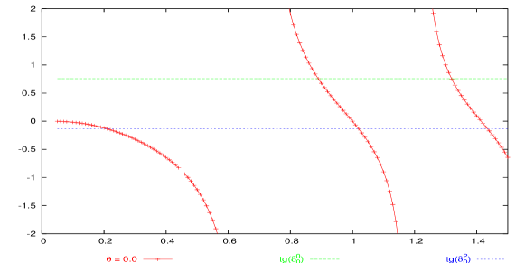
Figure 1: The red points represent $-\tan{\phi(\theta,Q)}$ as function of $Q$ for $\theta=0.0$. The different branches are the two–particle eigenvalues curves. The straight lines are the tangents of the scattering phases of two pions, having isospin $I=0$ or $I=2$, computed in chiral perturbation theory at the kaon mass.

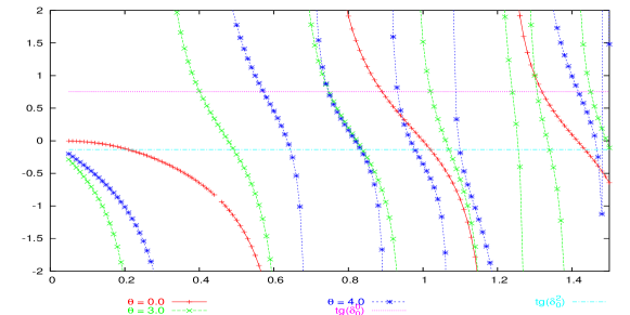
Figure 2: The points represent $-\tan{\phi(\theta,Q)}$ as functions of $Q$ for different values of $\theta$. The case $\theta=2.5$ is not shown to help the eye. The straight lines are the tangents of the scattering phases of two pions, having isospin $I=0$ or $I=2$, computed in chiral perturbation theory at the kaon mass.

In fig. 1 we show the opposite of $\tan\left[\phi(\theta,Q)\right]$ for the particular choice $\theta=0.0$. The points in which this function coincide with the function $\tan{\delta_{0}(q)}$ at fixed $\theta$ and $L$ represent the two–particle eigenvalues on the given volume but, in the following we want to perform a slightly different phenomenological analysis:

• we fix the energy of the two particle state so that $q=\overline{q}$
  

• we compute the corresponding scattering phase $\delta_{0}(\overline{q})$ (using the one–loop chiral perturbation theory results for these quantities [15, 16, 17, 18, 19])
  

• we find the values of $\overline{Q}_{n}(\theta)$ such that the condition

  $$\tan{\delta_{0}(\overline{q})}=-\tan{\phi(\theta,\overline{Q})}$$ (54)

  is satisfied.
  

• the volume $\overline{L}_{n}(\theta)$ on which the $n^{\mbox{th}}$ two–particle eigenvalue is equal to $\overline{q}$ is computed according to

  $$\overline{L}_{n}(\theta)=2\pi\frac{\overline{Q}_{n}(\theta)}{\overline{q}}$$ (55)

Following these steps we are able to find for each value of $\theta$ the finite volumes on which a given energy level of a two–pion state equals the kaon mass. In ref. [4] the authors have not considered the possibility of having $\theta\neq 0$ and their analysis, that we reproduce in fig. 1, gives the following results

$$I=0\qquad\qquad\overline{Q}_{1}(0)=0.89\qquad\qquad\overline{L}_{1}(0)=5.34\mbox{ fm}$$

$$I=2\qquad\qquad\overline{Q}_{1}(0)=1.02\qquad\qquad\overline{L}_{1}(0)=6.09\mbox{ fm}$$ (56)

i.e. the numerical simulations should be performed on volumes of order of $5.5$ fm that, in the case of unquenched calculations, could be too large even for the next–generation super computers. In fig. 2 we repeat the same analysis for other allowed values of $\theta$. As can be seen a careful choice of the “Bloch angle” shifts the position of the first eigenvalue curves at lower values of $Q$ and consequently, being $q$ fixed, at lower values of the physical volume.

$\theta$	$I$	$\overline{Q}_{1}$	$L_{1}$
0.0	0	0.890	5.34
0.0	2	1.015	6.09
2.5	0	0.295	1.78
2.5	2	0.415	2.49
3.0	0	0.400	2.40
3.0	2	0.490	2.94
4.0	0	0.569	3.41
4.0	2	0.645	3.86

Table 1: Volumes on which the energy of the first eigenvalue two–pion state equals the $K$–meson mass. $I$ is the isospin of the state.

The resulting volumes corresponding to our particular choices of $\theta$ are given in tab. 1. As can be seen the volumes to be simulated are of the order of $3$ fm that are accessible on present super–computers. A similar analysis can be repeated for all the allowed values of $\theta$ ($0\leq\theta_{i}<2\pi$) in order to obtain a longer sequence of finite volumes of growing physical sizes on which the decay amplitudes can be computed at the physical point. As already pointed out in the previous section, the size of the finite volume corrections to eq. (42) and to eq. (50) can be quantified by repeating the calculations on this sequence of volumes and by studying the functional dependence of the results upon the box extension.

6 Conclusions

In this work we have studied the spectrum of a two particle state on a finite volume with Bloch’s boundary conditions.

We have found a quantization condition that generalizes a result previously obtained by Lüscher in the case of periodic boundary conditions and that relates the energy eigenvalues of a two–particle system on a finite volume with their infinite volume scattering phases. The formula is valid up to exponentially small finite volume corrections and allows the calculations of the scattering phases at small physical momenta by calculating, for example on the lattice, the energy spectrum of the two–particle state on volumes of the order of $3$ fm.

From our quantization condition it follows straightforwardly a generalization of the Lellouch–Lüscher formula that connects the finite volume amplitudes for the decays of a kaon into two pions with the corresponding quantities in the infinite volume. We have argued that the decay amplitudes can be obtained simulating on the lattice finite volumes of different physical extensions in order to quantify the size of the residual finite volume corrections and thus to obtain results with a phenomenologically relevant accuracy.

Appendix A Derivation of the partial wave expansion of the greenian

In this appendix we derive the partial wave expansion of the greenian of eq. (29) that we have used to derive the generalized Lüscher’s quantization conditions. We start by recalling the well known Neumann’s expansion of the Green’s function

$$-\frac{1}{4\pi}\frac{e^{iq\left\|{{\vec{r}}-{\vec{r}}^{\prime}}\right\|}}{\left\|{{\vec{r}}-{\vec{r}}^{\prime}}\right\|}=q\sum_{lm}j_{l}(qr)Y_{lm}(\hat{r})\left[n_{l}(qr^{\prime})-ij_{l}(qr^{\prime})\right]Y^{*}_{lm}(\hat{r}^{\prime})$$ (57)

The previous relation is valid provided that $r<r^{\prime}$ otherwise one has to exchange ${\vec{r}}$ and ${\vec{r}}^{\prime}$ in the right–hand side. We insert the Neumann expansion in the expression for the greenian that we report below for clarity

$$g_{\vec{k}}({\vec{r}}-{\vec{r}}_{0};q)=-\frac{1}{4\pi}\sum_{{\vec{n}}\in{\bf Z}^{3}}{e^{i{\vec{k}}\cdot{\vec{n}}L}\frac{e^{iq\left\|{{\vec{r}}-{\vec{r}}_{0}-{\vec{n}}L}\right\|}}{\left\|{{\vec{r}}-{\vec{r}}_{0}-{\vec{n}}L}\right\|}}$$ (58)

For convenience we separate out the term with ${\vec{n}}={\vec{0}}$ from the remaining terms and we use the Neumann expansion identifying ${\vec{r}}^{\prime}$ with ${\vec{r}}_{0}$ in the first case and with ${\vec{n}}L$ in the second case. We end up with

$$g_{\vec{k}}( {\vec{r}}-{\vec{r}}_{0};q)=$$ (59)

$$=-\frac{1}{4\pi}\frac{\cos\left\|{{\vec{r}}-{\vec{r}}_{0}}\right\|}{\left\|{{\vec{r}}-{\vec{r}}_{0}}\right\|}+\sum_{lm}{D_{lm}({\vec{k}},q)\ j_{l}(q\left\|{{\vec{r}}-{\vec{r}}_{0}}\right\|)\ Y_{lm}(\widehat{{\vec{r}}-{\vec{r}}_{0}})}$$

where the so called reduced structure coefficients are given by

$$D_{lm} ({\vec{k}},q)=$$ (60)

$$=\sum_{{\vec{n}}\in{\bf Z}^{3}-\left\{{\vec{0}}\right\}}{e^{i{\vec{k}}\cdot{\vec{n}}L}Y_{lm}(\hat{n})\left[n_{l}(qnL)-ij_{l}(qnL)\right]}\,-i\frac{q}{\sqrt{4\pi}}\delta_{l0}\delta_{m0}$$

There are many different, although equivalent from the mathematical point of view, ways to express the reduced structure coefficients some of which are more convenient than the previous relation for a numerical computation of these quantities. In the appendix B we derive an expression suitable for the numerical calculation.

We need to recall another well known identity that can be easily proved by using the expansion in spherical harmonics of a plane wave (see eq. (71))

$$i^{JK}j_{J}(qR) Y_{JK}(\hat{R})=$$ (61)

$$=4\pi\sum_{lm,l^{\prime}m^{\prime}}{i^{l-l^{\prime}}C_{JK;lm,l^{\prime}m^{\prime}}\ j_{l}(qr)\ j_{l^{\prime}}(qr_{0})\ Y_{lm}(\hat{r})Y_{l^{\prime}m^{\prime}}(\hat{r}_{0})}$$

where we have called $R=\left\|{{\vec{r}}-{\vec{r}}_{0}}\right\|$ and we have introduced the Gaunt coefficients (see eq. (31) in the text)

$$C_{JK;lm,l^{\prime}m^{\prime}}=\int{d\Omega_{\vec{k}}Y_{JK}(\hat{k})Y_{lm}^{*}(\hat{k})Y_{l^{\prime}m^{\prime}}(\hat{k})}$$ (62)

Inserting the identity of eq. (61) in the partial wave expansion of the greenian as given in eq. (59) we are able to rewrite this expansion in the same form of eq. (29) that we have used in the text to derive the quantization conditions, i.e.

$$g_{\vec{k}}({\vec{r}}-{\vec{r}}_{0};q) = q\sum_{lm}{j_{l}(qr)\ Y_{lm}(\hat{r})n_{l}(qr_{0})\ Y_{lm}^{*}(\hat{r}_{0})}$$ (63)

$$+ \sum_{lml^{\prime}m^{\prime}}{j_{l}(qr)\ Y_{lm}(\hat{r})\ \Gamma_{lm,l^{\prime}m^{\prime}}({\vec{k}},q)\ j_{l^{\prime}}(qr_{0})\ Y_{l^{\prime}m^{\prime}}(\hat{r}_{0})}$$

where $r<r_{0}<nL\neq 0$, and we have introduced the structure coefficients

$$\Gamma_{lm,l^{\prime}m^{\prime}}({\vec{k}},q)=4\pi\ i^{l-l^{\prime}}\sum_{JK}{i^{-J}D_{JK}({\vec{k}},q)\ C_{JK;lm,l^{\prime}m^{\prime}}}$$ (64)

Appendix B Structure coefficients calculation

In this appendix we derive a mathematical expression useful for the numerical calculation of the structure coefficients. From eq. (64) we realize that the non trivial part of this problem consists in the calculation of the reduced structure coefficients. In the following we are going to derive an expression of the reduced structure coefficients, different from that already given in eq. (60), in order to handle a formula suitable for the numerical evaluation. We start again from the greenian definition

$$g_{\vec{k}}({\vec{R}};q)=-\frac{1}{4\pi}\sum_{{\vec{n}}\in{\bf Z}^{3}}{e^{i{\vec{k}}\cdot{\vec{n}}L}\frac{e^{iq\left\|{{\vec{R}}-{\vec{n}}L}\right\|}}{\left\|{{\vec{R}}-{\vec{n}}L}\right\|}}$$ (65)

having the aim to express it in the reciprocal space. To this end we recall the following well known identities

$$\frac{1}{(2\pi)^{3}}\int{d{\vec{x}}\ e^{i({\vec{p}}_{1}-{\vec{p}}_{2})\cdot{\vec{x}}}}=\delta({\vec{p}}_{1}-{\vec{p}}_{2})$$ (66)

$$\frac{1}{L^{3}}\sum_{{\vec{p}}_{m}}{e^{i{\vec{p}}_{m}\cdot{\vec{x}}}}=\sum_{{\vec{n}}\in{\bf Z}^{3}}{\delta({\vec{x}}-{\vec{n}}L)\ ,\qquad{\vec{p}}_{m}=\frac{2\pi}{L}{\vec{m}}}$$ (67)

$$\lim_{\varepsilon\rightarrow 0^{+}}{\frac{1}{(2\pi)^{3}}\int{d{\vec{p}}\ \frac{e^{i{\vec{p}}\cdot{\vec{x}}}}{p^{2}-(q^{2}+i\varepsilon)}}}=\frac{1}{(4\pi)}\frac{e^{iqx}}{x}$$ (68)

that allow us to write the following chain of equalities

$$g_{\vec{k}}({\vec{R}};q) = -\frac{1}{(2\pi)^{3}}\lim_{\varepsilon\rightarrow 0^{+}}{\sum_{{\vec{n}}\in{\bf Z}^{3}}{e^{i{\vec{k}}\cdot{\vec{n}}L}\ \int{d{\vec{p}}\ \frac{e^{i{\vec{p}}\cdot({\vec{R}}-{\vec{n}}L)}}{p^{2}-(q^{2}+i\varepsilon)}}}}$$ (69)

$$= -\frac{1}{(2\pi)^{3}}\lim_{\varepsilon\rightarrow 0^{+}}{\int{d{\vec{p}}\ \frac{e^{i{\vec{p}}\cdot{\vec{R}}}}{p^{2}-(q^{2}+i\varepsilon)}\ \sum_{{\vec{n}}\in{\bf Z}^{3}}{e^{i({\vec{k}}-{\vec{p}})\cdot{\vec{n}}L}}}}$$

$$= -\lim_{\varepsilon\rightarrow 0^{+}}{\int{d{\vec{p}}\ \frac{e^{i{\vec{p}}\cdot{\vec{R}}}}{p^{2}-(q^{2}+i\varepsilon)}\ \frac{1}{(2\pi)^{3}}\int{d{\vec{x}}\sum_{{\vec{n}}\in{\bf Z}^{3}}{\delta({\vec{x}}-{\vec{n}}L)e^{i({\vec{k}}-{\vec{p}})\cdot{\vec{x}}}}}}}$$

$$= -\lim_{\varepsilon\rightarrow 0^{+}}{\frac{1}{L^{3}}\sum_{{\vec{p}}_{m}}{\int{d{\vec{p}}\ \frac{e^{i{\vec{p}}\cdot{\vec{R}}}}{p^{2}-(q^{2}+i\varepsilon)}\ \frac{1}{(2\pi)^{3}}\int{d{\vec{x}}e^{i({\vec{k}}+{\vec{p}}_{m}-{\vec{p}})\cdot{\vec{x}}}}}}}$$

$$= -\lim_{\varepsilon\rightarrow 0^{+}}{\frac{1}{L^{3}}\sum_{{\vec{p}}_{m}}{\int{d{\vec{p}}\ \frac{e^{i{\vec{p}}\cdot{\vec{R}}}}{p^{2}-(q^{2}+i\varepsilon)}\ \delta({\vec{k}}+{\vec{p}}_{m}-{\vec{p}})}}}$$

$$= -\frac{1}{L^{3}}\sum_{{\vec{p}}_{m}}{\frac{e^{i({\vec{k}}+{\vec{p}}_{m})\cdot{\vec{R}}}}{({\vec{k}}+{\vec{p}}_{m})^{2}-q^{2}}}$$

i.e., the greenian expression in the reciprocal space is given by

$$g_{\vec{k}}({\vec{R}};q)=-\frac{1}{L^{3}}\sum_{{\vec{q}}_{m}}{\frac{e^{i{\vec{q}}_{m}\cdot{\vec{R}}}}{{\vec{q}}_{m}^{2}-q^{2}}\ ,\qquad{\vec{q}}_{m}={\vec{k}}+\frac{2\pi}{L}{\vec{m}}}$$ (70)

We are now ready to derive an expression for the KKR reduced structure coefficients in the reciprocal space. To this end we need to recall the identity expressing a plane wave as an expansion in spherical harmonics

$$e^{i{\vec{q}}_{m}\cdot{\vec{R}}}=4\pi\sum_{lm}{i^{l}j_{l}(q_{m}R)\ Y_{lm}^{*}(\hat{q}_{m})\ Y_{lm}(\hat{R})}$$ (71)

so that the greenian can be expanded as follows

$$g_{\vec{k}}({\vec{R}};q)=\sum_{lm}{\left(-\frac{4\pi\ i^{l}}{L^{3}}\sum_{{\vec{q}}_{m}}{\frac{j_{l}(q_{m}R)}{j_{l}(qR)}\ \frac{Y_{lm}^{*}(\hat{q}_{m})}{{\vec{q}}_{m}^{2}-q^{2}}}\right)j_{l}(qR)\ Y_{lm}(\hat{R})}$$ (72)

In order to reproduce the same structure of eq. (59) we make the following observation

$$g_{\vec{k}}({\vec{R}};q) = g_{\vec{k}}({\vec{R}};q)-\frac{1}{4\pi}\frac{cos(qR)}{R}+\frac{1}{4\pi}\frac{cos(qR)}{R}$$ (73)

$$= g_{\vec{k}}({\vec{R}};q)-\frac{1}{4\pi}\frac{cos(qR)}{R}+\frac{q}{4\pi}\cot(qR)\ \frac{sin(qR)}{R}$$

$$= g_{\vec{k}}({\vec{R}};q)-\frac{1}{4\pi}\frac{cos(qR)}{R}+\frac{q}{4\pi}\cot(qR)\ j_{0}(qR)$$

inserting the last identity in eq. (72) we end up with

$$g_{\vec{k}}({\vec{R}};q)=-\frac{1}{4\pi}\frac{cos(qR)}{R}+\sum_{lm}{D_{lm}({\vec{k}},q;R)j_{l}(qR)\ Y_{lm}(\hat{R})}$$ (74)

where we have obtained

$$D_{lm}({\vec{k}},q;R)=-\frac{4\pi i^{l}}{L^{3}}\sum_{{\vec{q}}_{m}}{\frac{j_{l}(q_{m}R)}{j_{l}(qR)}\ \frac{Y_{lm}^{*}(\hat{q}_{m})}{{\vec{q}}_{m}^{2}-q^{2}}}+\frac{q}{\sqrt{4\pi}}\cot(qR)\ \delta_{l0}\ \delta_{m0}$$ (75)

This expression requires some comments. First we want to note that

$$Y_{lm}^{*}(\hat{q}_{m})=Y_{lm}(\hat{q}^{\prime}_{m})\qquad{\vec{q}}_{m}=(q_{m}^{1},q_{m}^{2},q_{m}^{3})\qquad{\vec{q}}^{\prime}_{m}=(q_{m}^{1},-q_{m}^{2},q_{m}^{3})$$ (76)

so that, being the rest of the sum argument a function of the modulus of ${\vec{q_{m}}}$ only, we can write

$$D_{lm}({\vec{k}},q;R)=-\frac{4\pi i^{l}}{L^{3}}\sum_{{\vec{q}}_{m}}{\frac{j_{l}(q_{m}R)}{j_{l}(qR)}\ \frac{Y_{lm}(\hat{q}_{m})}{{\vec{q}}_{m}^{2}-q^{2}}}+\frac{q}{\sqrt{4\pi}}\cot(qR)\ \delta_{l0}\ \delta_{m0}$$ (77)

The second observation concerns the $R$–dependence of the reduced structure coefficients. Indeed, by the comparison of eq. (60) with the previous equation we learn that this functional dependence is fictitious. This can be also understood by a careful analysis of eq. (74). We know that the term

$$n_{0}(qR)=\frac{cos(qR)}{qR}$$ (78)

satisfies by its own the equation

$$\left(\triangle+q^{2}\right)n_{0}(qR)=-\frac{4\pi}{q}\delta({\vec{R}})$$ (79)

so that the remaining terms of the sum in eq. (74) must be regular solutions of the homogeneous Helmholtz’s equation. A general solution of this kind can be expressed as a linear combination of the form

$$\hat{g}_{\vec{k}}({\vec{R}};q)=\sum_{lm}{D_{lm}({\vec{k}},q)j_{l}(qR)\ Y_{lm}(\hat{R})}$$ (80)

where the $D_{lm}({\vec{k}},q)$ are constants by respect to $R$. We also learn from textbooks on mathematical functions that near the origin the spherical Bessel functions deal as

$$j_{l}(qR)\stackrel{{\scriptstyle R\rightarrow 0}}{{\longrightarrow}}(qR)^{l}$$ (81)

The fictitious $R$–dependence of the reduced structure coefficients as given in eq. (77) can be eliminated taking the limit for $R$ that goes to zero and using the previous equation.

One has to consider eq. (77) as a properly regulated form of the KKR reduced structure coefficients and think to the following

$$D_{lm}({\vec{k}},q)=-\frac{4\pi i^{l}}{q^{l}L^{3}}\sum_{{\vec{q}}_{m}}{\frac{q_{m}^{l}\ Y_{lm}(\hat{q}_{m})}{{\vec{q}}_{m}^{2}-q^{2}}}+\frac{\delta_{l0}\ \delta_{m0}}{\sqrt{4\pi}}\lim_{R\rightarrow 0}{\frac{1}{R}}$$ (82)

as a formal expression of the same objects.

B.1 Ewald’s sums

In ref. [13] Kohn and Rostoker considered a method particularly convenient from the numerical point of view to evaluate the reduced structure coefficients. They pointed out that, following a prescription due to Ewald [20], the sum

$$S(x)=\sum_{{\vec{q}}_{m}}{\frac{j_{l}(q_{m}R)\ Y_{lm}(\hat{q}_{m})}{q_{m}^{2}-q_{2}}\ e^{\frac{q^{2}-q_{m}^{2}}{x}}}$$ (83)

approximate the needed result $S(\infty)$ with an exponential vanishing error. In ref. [21] the original observation of Kohn and Rostoker was further refined by Ham and Segall. They first recall two identities both due to Ewald; the first one is

$$\frac{e^{iq\left\|{{\vec{R}}-{\vec{n}}L}\right\|}}{\left\|{{\vec{R}}-{\vec{n}}L}\right\|}=\lim_{\varepsilon\rightarrow 0}{\frac{2}{\sqrt{\pi}}\int_{0}^{\infty}{dx\ e^{-({\vec{R}}-{\vec{n}}L)^{2}x^{2}+\frac{q^{2}+i\varepsilon}{4x^{2}}}}}$$ (84)

The second identity can be proved as done before to express the greenian in the reciprocal space starting from its expression in the direct space and states

$$\sum_{{\vec{n}}\in{\bf Z}^{3}}{e^{-({\vec{R}}-{\vec{n}}L)^{2}x^{2}+i{\vec{k}}\cdot({\vec{n}}L-{\vec{R}})}=\frac{(\sqrt{\pi})^{3}}{(Lx)^{3}}\sum_{{\vec{p}}_{m}}{e^{i{\vec{p}}_{m}\cdot{\vec{R}}-\frac{q_{m}^{2}}{4x^{2}}}}}\qquad{\vec{p}}_{m}=\frac{2\pi}{L}{\vec{m}}$$ (85)

We now start again from the expression of the greenian in the direct space as given in eq. (65) and write, by using the first identity (84),

$$g_{\vec{k}}({\vec{R}};q)=-\frac{1}{2(\sqrt{\pi})^{3}}\lim_{\varepsilon\rightarrow 0}{\sum_{{\vec{n}}\in{\bf Z}^{3}}{\int_{0}^{\infty}{dx\ e^{i{\vec{k}}\cdot{\vec{n}}L-({\vec{R}}-{\vec{n}}L)^{2}x^{2}+\frac{q^{2}+i\varepsilon}{4x^{2}}}}}}$$ (86)

then we split the integration domain in $\left[0,\frac{\sqrt{\eta}}{2}\right]$ and $\left[\frac{\sqrt{\eta}}{2},\infty\right]$, where $\eta$ is a positive arbitrary constant. The greenian can be thus re-expressed as the sum of two terms

$$g_{\vec{k}}({\vec{R}};q)=g_{\vec{k}}^{1}({\vec{R}};q)+g_{\vec{k}}^{2}({\vec{R}};q)$$ (87)

where, performing the integration in the first term and using the identity of eq. (85) in the second one, we obtain

$$g_{\vec{k}}^{1}({\vec{R}};q) = \frac{1}{L^{3}}\sum_{{\vec{q}}_{m}}{\frac{e^{i{\vec{q}}_{m}\cdot{\vec{R}}+\frac{q^{2}-q_{m}^{2}}{\eta}}}{q^{2}-q_{m}^{2}}}$$

$$g_{\vec{k}}^{2}({\vec{R}};q) = -\frac{1}{2(\sqrt{\pi})^{3}}\sum_{{\vec{n}}\in{\bf Z}^{3}}{\int_{\frac{\sqrt{\eta}}{2}}^{\infty}{dx\ e^{i{\vec{k}}\cdot{\vec{n}}L-({\vec{R}}-{\vec{n}}L)^{2}x^{2}+\frac{q^{2}}{4x^{2}}}}}$$ (88)

These series are absolutely convergent for any finite $\eta>0$ and each term is an analytic function of $q$ throughout the complex plane except at the simple pole $q^{2}=q_{m}^{2}$. Expanding termwise both $g_{\vec{k}}^{1}$ and $g_{\vec{k}}^{2}$ in spherical harmonics by respect to ${\vec{R}}$, taking the limit $R\rightarrow 0$, and comparing the result with the definition of the reduced structure coefficients, we find

$$D_{lm}({\vec{k}},q)=D_{lm}^{1}({\vec{k}},q)+D_{lm}^{2}({\vec{k}},q)+D_{lm}^{3}({\vec{k}},q)$$ (89)

where

$$D_{lm}^{1}({\vec{k}},q) = \frac{4\pi}{L^{3}q^{l}}\ e^{\frac{q^{2}}{\eta}}\ \sum_{{\vec{q}}_{m}}{\frac{q_{m}^{l}}{q^{2}-q_{m}^{2}}\ Y_{lm}(\hat{q}_{m})\ e^{-\frac{q_{m}^{2}}{\eta}}}$$

$$D_{lm}^{2}({\vec{k}},q) = -\frac{2^{l+1}L^{l}i^{l}}{q^{l}\sqrt{\pi}}\sum_{{\vec{n}}\in{\bf Z}^{3}-\left\{{\vec{0}}\right\}}{n^{l}\ e^{i{\vec{k}}\cdot{\vec{n}}L}\ Y_{lm}(\hat{n})\ \int_{\frac{\sqrt{\eta}}{2}}^{\infty}{dx\ x^{2l}\ e^{-(x{\vec{n}}L)^{2}+\frac{q^{2}}{4x^{2}}}}}$$

$$D_{lm}^{3}({\vec{k}},q) = -\delta_{l0}\ \delta_{m0}\ \frac{\sqrt{\eta}}{2\pi}\sum_{s=0}^{\infty}{\frac{q^{2s}}{\eta^{s}}\ \frac{1}{s!(2s-1)}}$$ (90)

In order to make more explicit the dependence of the reduced structure coefficients upon the volume let us define

$$d_{lm}(\theta,Q) = LD_{lm}({\vec{k}},q)$$ (91)

$$= d_{lm}^{1}(\theta,Q)+d_{lm}^{2}(\theta,Q)+d_{lm}^{3}(\theta,Q)$$

and rewrite eqs. (90) as follows

$$d_{lm}^{1}(\theta,Q) = \frac{i^{l}}{\pi Q^{l}}\ e^{\frac{Q^{2}}{\eta^{\prime}}}\ \sum_{{\vec{Q}}_{m}}{\frac{Q_{m}^{l}\ Y_{lm}(\hat{Q}_{m})}{Q^{2}-Q_{m}^{2}}\ e^{-\frac{Q_{m}^{2}}{\eta^{\prime}}}}$$

$$d_{lm}^{2}(\theta,Q) = -\frac{4^{l+1}i^{l}\sqrt{\pi}}{Q^{l}}\sum_{{\vec{n}}\in{\bf Z}^{3}-\left\{{\vec{0}}\right\}}{(\pi n)^{l}e^{i{\vec{\theta}}\cdot{\vec{n}}}Y_{lm}(\hat{n})\int_{\frac{\sqrt{\eta^{\prime}}}{2}}^{\infty}{dxx^{2l}e^{-(2\pi x{\vec{n}})^{2}+\frac{Q^{2}}{4x^{2}}}}}$$

$$d_{lm}^{3}(\theta,Q) = -\delta_{l0}\ \delta_{m0}\ \sqrt{\eta^{\prime}}\sum_{s=0}^{\infty}{\frac{Q^{2s}}{{\eta^{\prime}}^{s}}\ \frac{1}{s!(2s-1)}}$$ (92)

where we have substituted

$$Q=\frac{Lq}{2\pi}\qquad\qquad\qquad Q_{m}=\left\|{{\vec{m}}+\frac{{\vec{\theta}}}{2\pi}}\right\|$$ (93)

$${\vec{k}}=\frac{{\vec{\theta}}}{L}\qquad\qquad\qquad \eta^{\prime}=\left(\frac{L}{2\pi}\right)^{2}\eta$$ (94)

B.2 Incomplete Gamma Function

The computation of the reduced structure coefficients is complicated from the numerical point of view by the presence of an integral in the definition of $d_{lm}^{2}(\theta,Q)$. In order to simplify the numerical task let us recall the definition of the incomplete gamma function:

$$\Gamma(\alpha,y)=\int_{y}^{\infty}{dx\ x^{\alpha-1}e^{-x}}$$ (95)

using the incomplete gamma function, $d_{lm}^{2}(\theta,Q)$ can be rewritten in the following form

$$d_{lm}^{2}(\theta,Q)=-\frac{i^{l}\sqrt{\pi}}{Q^{l}}\times$$

$$\times\sum_{p}{\frac{Q^{2p}}{p!}\sum_{{\vec{n}}\in{\bf Z}^{3}-\left\{{\vec{0}}\right\}}{\frac{e^{i{\vec{\theta}}\cdot{\vec{n}}}}{(\pi n)^{l-2p+1}}\ Y_{lm}(\hat{n})\ \Gamma\left(l-p+\frac{1}{2},(\pi n)^{2}\eta^{\prime}\right)}}$$ (96)

The great advantage of this expression with respect to the one given in eq. (92) is that the incomplete gamma function can be computed numerically using a continued fraction representation:

$$\Gamma(\alpha,y)=\frac{e^{-y}\ y^{\alpha}}{x\;+\;\frac{1-\alpha}{1\;+\;\frac{1}{x\;+\;\frac{2-\alpha}{1\;+\;\frac{2}{x\;+\;\frac{3-\alpha}{1\;+\;\dots}}}}}}$$ (97)

References

- [1] D. Becirevic, Nucl. Phys. Proc. Suppl. 129-130 (2004) 34.
- [2] L. Maiani and M. Testa, Phys. Lett. B245 (1990) 585.
- [3] M. Ciuchini et al., Phys. Lett. B380 (1996) 353, hep-ph/9604240.
- [4] L. Lellouch and M. Luscher, Commun. Math. Phys. 219 (2001) 31, hep-lat/0003023.
- [5] M. Luscher, Commun. Math. Phys. 104 (1986) 177.
- [6] M. Luscher, Commun. Math. Phys. 105 (1986) 153.
- [7] M. Luscher, Nucl. Phys. B354 (1991) 531.
- [8] M. Luscher, Nucl. Phys. B364 (1991) 237.
- [9] C.J.D. Lin et al., Nucl. Phys. B619 (2001) 467, hep-lat/0104006.
- [10] G.M. de Divitiis, R. Petronzio and N. Tantalo, Phys. Lett. B595 (2004) 408, hep-lat/0405002.
- [11] M. Luscher and U. Wolff, Nucl. Phys. B339 (1990) 222.
- [12] J. Korringa, Physica (Utrecht) 13 (1947) 392.
- [13] W. Kohn and N. Rostoker, Phys. Rev. 94 (1954) 1111.
- [14] K. Rummukainen and S.A. Gottlieb, Nucl. Phys. B450 (1995) 397, hep-lat/9503028.
- [15] J. Gasser and H. Leutwyler, Phys. Lett. B125 (1983) 325.
- [16] J. Gasser and H. Leutwyler, Ann. Phys. 158 (1984) 142.
- [17] J. Gasser and H. Leutwyler, Nucl. Phys. B250 (1985) 465.
- [18] J. Gasser and U.G. Meissner, Phys. Lett. B258 (1991) 219.
- [19] M. Knecht et al., Nucl. Phys. B457 (1995) 513, hep-ph/9507319.
- [20] P. Ewald, Ann. Physik. 64 (1921) 253.
- [21] F.S. Ham and B. Segall, Phys. Rev. 124 (1961) 1786.