DESY 04-166     
ITEP-LAT/2004-17     
KANAZAWA-04-12     
Finite temperature QCD with two flavors of dynamical quarks on $24^{3}\times 10$ lattice

Abstract

We present results obtained in QCD with two flavors of non-perturbatively improved Wilson fermions at finite temperature on $16^{3}\times 8$ and $24^{3}\times 10$ lattices. We determine the transition temperature in the range of quark masses $0.6<m_{\pi}/m_{\rho}<0.8$ at lattice spacing a$\approx$0.1 fm and extrapolate the transition temperature to the continuum and to the chiral limits.

1 INTRODUCTION

In order to obtain predictions for the real world from lattice QCD, we have to extrapolate the lattice data to the continuum and to the chiral limits. Recently the Bielefeld group [1] and the CP-PACS collaboration [2] using different fermion actions obtained consistent values for the critical temperature $T_{c}$ in the chiral limit, albeit on rather coarse lattices at $N_{t}=4$ and 6. Edwards and Heller [3] determined $T_{c}$ for $N_{t}=4$, 6 using nonperturbatively improved Wilson fermions. We compute $T_{c}$ on finer lattices with $N_{t}=8$ and 10 with high statistics. Our results for $N_{t}=8$ were reported in Ref. [4].

2 SIMULATION

We use fermionic action for non-perturbatively improved Wilson fermions:

$$S_{F} = S^{o}_{F}-\frac{\rm i}{2}\kappa\,g\,c_{sw}a^{5}\sum\nolimits_{x}\bar{\psi}(x)\sigma_{\mu\nu}F_{\mu\nu}\psi(x),$$

where $S^{o}_{F}$ is the original Wilson action, $c_{sw}$ was calculated in [5].

Configurations are generated on $16^{3}\times 8$ ($\beta=5.2$ and $5.25$) and $24^{3}\times 10$ ($\beta=5.2$) lattices at various $\kappa$. The values of $\kappa$ and the corresponding number of configurations for $16^{3}\times 8$ and $24^{3}\times 10$ lattices can be found in Ref. [4] and Table 1, respectively. The number of configurations for $24^{3}\times 10$ lattice is not large enough and results for this lattice are preliminary. We use results obtained at T=0 to fix the scale. The contour plot of lines of constant $r_{0}/a$ and $m_{\pi}/m_{\rho}$ [6] is shown in Fig. 1.

$\kappa$	$0.1348$	$0.1352$	$0.1354$	$0.1355$
# conf.	$678$	$679$	$1,234$	$799$
$\kappa$	$0.1356$	$0.1358$	$0.1360$
# conf.	$2,429$	$480$	$617$

Table 1:Simulation statistics on $24^{3}\times 10$.

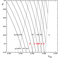
Figure 1: The lines of constant $r_{0}/a$ and $m_{\pi}/m_{\rho}$ at $T=0$. Crosses correspond to parameters used in simulations of $24^{3}\times 10$ lattice.

3 CRITICAL TEMPERATURE

We use the Polyakov loop susceptibility to determine the transition point. The critical value of $\kappa$ turns out to be $\kappa_{t}$=0.1354. Using $r_{0}$=0.5 fm and interpolating $r_{0}/a$ to the critical point, we obtain for the crtical temperature:

$T_{c}=196(4)$MeV,   ${m_{\pi}/m_{\rho}}=0.64(3)$

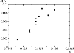
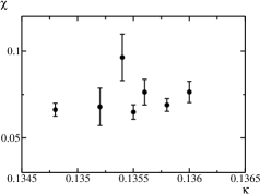
Figure 2: Polyakov loop (top) and its susceptibility (bottom) at $\beta=5.2$ on $24^{3}\times 10$.

4 CONTINUUM AND CHIRAL LIMITS

At small enough lattice spacing and quark mass one can extrapolate the critical temperature $T_{c}$ to the continuum and the chiral limits using formula:

$$T_{c}r_{0}=T_{c}^{m_{q},a\to 0}r_{0}+C_{a}({a\over r_{0}})^{2}+C_{q}({1\over\kappa}-{1\over\kappa_{c}})^{{1\over\beta\delta}}\,,$$

where $T_{c}^{m_{q},a\to 0}$ corresponds to the extrapolated value of the critical temperature and $\beta$ and $\delta$ are critical indices.

We make an attempt to fit four values for $T_{c}r_{0}$ (see Table 3), obtained at rather large quark masses, to estimate the parameters in this extrapolation expression.

$T_{c}r_{0}$	$a/r_{0}$	$\beta$	$\kappa_{t}$	$L_{t}$
$0.50(1)$	$0.201(4)$	5.2	0.1354	10	prelim.
$0.53(1)$	$0.234(4)$	5.2	0.1345	8	Ref. [4]
$0.56(1)$	$0.225(4)$	5.25	0.1341	8	Ref. [4]
$0.57(2)$	$0.29(1)$	5.2	0.1330	6	Ref. [3]

Table 3:Available data for $T_{c}r_{0}$.

${1\over\beta\delta}$	$T_{c}r_{0}$	$C_{a}$	$C_{q}$	$\chi^{2}/dof$	order
$0.54$	$0.44(2)$	$-0.9(5)$	$0.5(1)$	$0.26$	2nd
$1$	$0.51(3)$	$-1.3(7)$	$0.9(2)$	$0.13$	1st

Table 4:Fitting results.

We extrapolate the value of the critical temperature using different values of 0.54 and 1 as $1/\beta\delta$. If the transition in two-flavor QCD is second order, the transition is expected to belong to the universality class of the $3D$ $O(4)$ spin model with $1/\beta\delta$$\approx$0.54. If the transition is first order, then $1/\beta\delta$=1. Table 4 and Figs. 4, 5 present fitting results. We get the critical temperature in the continuum and in the chiral limits.

In the case of $1/\beta\delta$$=$0.54:

$$T_{c}^{m_{q},a\to 0}=174(8)~{}\mbox{MeV}\,.$$ (1)

This value agrees with values obtained in Refs.[1, 2].

In the case of $1/\beta\delta$=1:

$$T_{c}^{m_{q},a\to 0}=201(12)~{}\mbox{MeV}\,.$$ (2)

Although some lattice studies [1, 2] indicate second order chiral transition in two-flavor QCD, there are also results [7] supporting first order transition. Results of our fits do not allow to discriminate between first and second order transitions because of rather large errors in $T_{c}r_{0}$ values.

5 CONCLUSIONS

We determined the critical temperature in full QCD on $24^{3}\times 10$ lattice at $\beta=5.2$ with $N_{f}=2$ clover fermions using Polyakov loop susceptibility. Our results are in agreement with the results of other groups, as it is shown in Fig. 3. We extrapolate the critical temperature $T_{c}$ to the continuum and the chiral limits both in cases of first and second order transition. The extrapolation results are given by (1) and (2). We are continuing simulations on $24^{3}\times 10$ lattice to get better precision of $T_{c}$ value on this lattice.

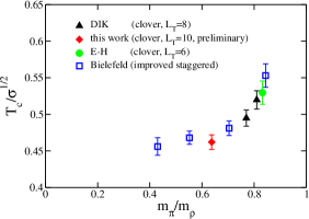
Figure 3: $T_{c}/\sqrt{\sigma}$ as a function of $m_{\pi}/m_{\rho}$. The circle and squares show results of [3] and [1] respectively. The diamond and triangles correspond to our data.

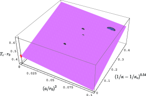
Figure 4: $T_{c}r_{0}$ as a function of lattice spacing and quark mass if the second order phase transition is realized. Best fit is shown by the plane.

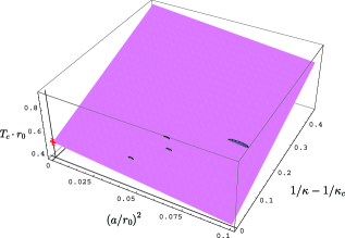
Figure 5: The same as in Fig.4 but for the first order phase transition.

6 ACKNOWLEDGEMENTS

This work is supported by the SR8000 Supercomputer Project of High Energy Accelerator Research Organization (KEK). A part of numerical measurements has been done using NEC SX-5 at Research Center for Nuclear Physics (RCNP) of Osaka University. The numerical simulations of this work were done using RSCC computer clusters in RIKEN. We wish to acknowledge the support of the computer center at RIKEN. VGB, MNC and MIP are supported by grants RFBR 02-02-17308, 04-02-16079, RFBR-DFG-03-02-04016, DFG-RFBR 436 RUS 113/739/0, INTAS-00-00111, CRDF award RPI-2364-MO-02 and MK-4019.2004.2, A.A.S. is supported by grant Scient.school grant 2052-2003.1. T.S. is supported by JSPS Grant-in-Aid for Scientific Research on Priority Areas 13135210 and (B) 15340073.

References

- [1] F. Karsch, A. Peikert, E. Laermann, Nucl. Phys. B605 (2001) 579.
- [2] A. Ali Khan et al., (CP-PACS), Phys. Rev. D63 (2001) 034502.
- [3] R. G. Edwards, U. M. Heller, Phys. Lett. B462 (1999) 132.
- [4] V. Bornyakov et al., hep-lat/0401014
- [5] K. Jansen and R. Sommer (ALPHA collaboration), Nucl. Phys. B530 (1998) 185.
- [6] S. Booth et al., Phys. Lett. B519 (2001) 229.
- [7] M. D’Elia et al., hep-lat/0408008